An Anisotropic Interaction Model for Simulating Fingerprints
Abstract.
Evidence suggests that both the interaction of so-called Merkel cells and the epidermal stress distribution play an important role in the formation of fingerprint patterns during pregnancy. To model the formation of fingerprint patterns in a biologically meaningful way these patterns have to become stationary. For the creation of synthetic fingerprints it is also very desirable that rescaling the model parameters leads to rescaled distances between the stationary fingerprint ridges. Based on these observations, as well as the model introduced by Kücken and Champod we propose a new model for the formation of fingerprint patterns during pregnancy. In this anisotropic interaction model the interaction forces not only depend on the distance vector between the cells and the model parameters, but additionally on an underlying tensor field, representing a stress field. This dependence on the tensor field leads to complex, anisotropic patterns. We study the resulting stationary patterns both analytically and numerically. In particular, we show that fingerprint patterns can be modeled as stationary solutions by choosing the underlying tensor field appropriately.
1. Introduction
Large databases are required for developing, validating and comparing the performance of fingerprint indexing and identification algorithms. The goal of these algorithms is to search and find a fingerprint in a database (or providing the search result that the query fingerprint is not stored in that database). The database sizes for fingerprint identification can vary between several thousand fingerprints e.g. watchlists in border crossing scenarios or hundreds of millions of fingerprints in case of the national biometric ID programme of India.
Clearly, fingerprint identification is of great importance in forensic science and is increasingly used in biometric applications. Unfortunately, collecting databases of real fingerprints for research purposes is usually very cost-intensive, requires time and effort, and in many countries, it is constrained by laws addressing important aspects such as data protection and privacy. Therefore, it is very desirable to avoid all these disadvantages by simulating large fingerprint databases on a computer.
The creation of synthetic fingerprint images is of great interest to the community of biometric and forensic researchers, as well as practitioners. The SFinGe method [13] has been proposed to this end by Cappelli et al. in 2000. This method can produce fingerprint images which look realistic enough to deceive attendees of a pattern recognition conference, however, systematic differences between real fingerprints and synthetic images by SFinGE regarding the minutiae pattern have been found which allow to distinguish between the two [32]. Recently, the realistic fingerprint creator (RFC) [38] has been suggested to overcome the issue of unrealistic minutiae distributions. SFinGe and RFC are both based on Gabor filters [31] for image creation. A different approach to fingerprint creation has been introduced by Kücken and Champod in [42]. They strive to directly model the process of fingerprint pattern formation as it occurs in nature and their approach is inspired by existing knowledge from biology, anatomy and dermatology. Two commonalities of Gabor filters based and biology-inspired approaches are that both start with random initial conditions and both perform changes in an iterative fashion. Kücken and Champod suggest a model describing the formation of fingerprint patterns over time based on the interaction of certain cells and mechanical stress in the epidermis [39].
In principle, a nature-inspired model nourishes the hope of producing more realistic fingerprints and potentially also to gain insights into the process of natural fingerprint pattern formation. An extensive literature [23, 24, 39, 42, 44, 45, 50] in the biological community suggests that fingerprint patterns are formed due to the interaction of mechanical stress, trophic factors from incoming nerves and interactions between so-called Merkel cells. Merkel cells are epidermal cells that appear in the volar skin at about the 7th week of pregnancy. From that time onward they start to multiply and organise themselves in lines exactly where the primary ridges arise [42]. Kücken and Champod [42] model this pattern formation process on a domain as the rearrangement of Merkel cells from a random initial configuration into roughly parallel ridges along the lines of smallest compressive stress. However, the resulting patterns do not seem to be stationary which is desirable for describing the formation of fingerprints accurately.
Motivated by their approach we propose a general class of evolutionary particle models with an anisotropic interaction force in two space dimensions where the form of the interaction forces is inspired by biology. This class of models can be regarded as an biology-inspired adaptation of the Kücken-Champod model [42]. In [11] a generalization of the Kücken-Champod model is proposed and its stationary states are studied both analytically and numerically in the spatially homogeneous case.
In this work, we consider interacting particles whose positions , at time satisfy
| (1.1) |
equipped with initial data . The term in (1.1) denotes the force which a particle at position exerts on a particle at position . This force depends on an underlying stress tensor field at location . The existence of such a tensor field is based on the experimental results in [41] where an alignment of the particles along the local stress lines is observed. We define the tensor field by the directions of smallest stress at location by a unit vector field and introduce a corresponding orthonormal vector field , representing the directions of largest stress. Then the force is given by
| (1.2) |
for coefficient functions and .
In previous works on the Kücken-Champod model [42] and its generalization [11] a dynamical system of ordinary differential equations of the form (1.1) was considered where the force that particle exerts on particle is given by
| (1.3) |
i.e. the sum of repulsion and attraction forces, and , respectively. Here, the attraction force depends on the underlying tensor field at , modeling the local stress field. The matrix encodes the direction of the fingerprint lines at , defined by
| (1.4) |
and orthonormal vector fields , . For studying the pattern formation with an underlying spatially homogeneous tensor field producing straight parallel ridges, e.g.
is considered [11]. The repulsion and attraction forces in the Kücken-Champod model [42] and its generalization in [11] are of the form
| (1.5) |
and
| (1.6) |
respectively. Note that the direction of the attraction force and hence also the direction of the total force are regulated by the parameter in the definition of the tensor field . The parameter introduces an anisotropy to the equation leading to complex, anisotropic patterns.
For the model (1.1) with interaction forces of the form (1.3) for repulsion and attraction force (1.5) and (1.6) reduces to a gradient flow
| (1.7) |
and for a radially symmetric interaction potential . The continuum equation associated with the isotropic particle model (1.7) is given by
where is the macroscopic velocity field. This continuum model, referred to as the aggregation equation has been studied extensively recently, mainly in terms of its gradient flow structure, the blow-up dynamics for fully attractive potentials and the rich variety of steady states, see [2, 3, 4, 5, 7, 8, 9, 12, 14, 15, 17, 19, 20, 21, 22, 27, 28, 43, 46, 47, 48, 49] and the references therein. There has been a trend recently to connect the microscopic and the macroscopic descriptions via kinetic modeling, see for instance [6, 18, 36] for different kinetic models in swarming, [30, 35] for the particle to hydrodynamics passage and [40] for the hydrodynamic limit of a kinetic model. It seems that not many results are currently available in the field of anisotropies. In [25, 26] anisotropy is modeled by adding weights to the interaction terms. One can show that the model in [25, 26] is related to our model if a tensor field is introduced as the velocity direction.
Fingerprint simulation results are shown for certain model parameters in [42] where the underlying tensor field is constructed based on fingerprint images using the NBIS package from the National Institute of Standards and Technology. However, [42] is purely descriptive, the choice of parameters is not discussed and the model (1.1) was not studied mathematically. The model (1.1) was studied analytically and numerically for the first time in [11]. Here, the authors justify why the particles align along the vector field lines provided the parameter is chosen sufficiently small so that the total force is purely repulsive along . Besides, the authors investigate the stationary states to the particle model (1.1) for a spatially homogeneous underlying tensor field where the chosen model parameters are consistent with the work of Kücken and Champod in [42]. For the simulation of fingerprints, however, non-homogeneous tensor fields have to be considered, making the analysis of the model significantly more difficult. No analytical results of the long-time behavior of (1.1) for non-homogeneous tensor fields are currently available. Besides, numerical results for the given model parameters and different non-homogeneous tensor fields are shown over time in [11] and one can clearly see that the resulting patterns are not stationary. The simulation results for realistic tensor fields for the simulation of fingerprints in [42] seem to be far away from being stationary too. This is illustrated in Figure 9 in [42] where snapshots of the solution are shown for a spatially homogeneous tensor field which should have been parallel lines for steady states. In the biological community, however, it is well-known that fingerprint patterns with their ridge lines and minutiae configuration are determined during pregnancy and remain the same during lifetime (as long as no fingerprint alterations occur). Hence, we are particularly interested in stationary solutions of the system (1.1).
The goal of this work is to develop an efficient algorithm for creating synthetic fingerprint patterns as stationary solutions of an evolutionary dynamical system of the form (1.1) as illustrated in Figure for the underlying tensor field in Figure .


As a first step we study the existence of stationary solutions to (1.1) for spatially homogeneous underlying tensor fields and extend these results to certain spatially inhomogeneous tensor fields. Based on these analytical results as well as the stability analysis of line patterns in [16] we can expect stable stationary patterns along the vector field . Since the solutions to the particle model (1.1) with the parameters suggested by Kücken and Champod do not seem to be stationary, we investigate the impact of the interaction forces on the resulting pattern formation numerically. In particular the size of the total attraction force plays a crucial role in the pattern formation. We adjust the model parameters accordingly and simulate fingerprints which seem to be close to being stationary, resulting in an extension of the numerical results in [11] for inhomogeneous tensor fields. Based on real fingerprint images as in Figure we determine the underlying tensor field with lines of smallest stress by extrapolating the direction field outside of the fingerprint image based on [33]. In Figure we overlay a mask of the original fingerprint image on the estimated tensor field with direction field and in Figure only the direction field is shown. Besides, we include a novel method for the generation of the underlying tensor fields in our numerical simulations which is based on quadratic differentials as a global model for orientation fields of fingerprints [37].
In the fingerprint community major features of a fingerprint, called minutiae, are of great interest. Examples include ridge bifurcation, i.e. a single ridge dividing into two ridges. We study how they evolve over time, both heuristically and numerically. Finally, we propose a new bio-inspired model for the creation of synthetic fingerprint patterns which not only allows us to simulate fingerprint patterns as stationary solution of the particle model (1.1) but also adjust the distances between the fingerprint lines by rescaling the model parameters. This is the first step towards modeling fingerprint patterns with specific features in the future.
Studying the model (1.1) and in particular its pattern formation result in a better understanding of the fingerprint pattern formation process. Due to the generality of the formulation of the anisotropic interaction model (1.1) this can be regarded as an important step towards understanding the formation of fingerprints and may be applicable to other anisotropic interactions in nature.
This work is organized as follows. In Section 2 the Kücken-Champod model [42] is introduced and we propose a new bio-inspired modeling approach. Section 3 deals with the existence of steady states to (1.1) for spatially homogeneous tensor fields and its extension to locally spatially homogeneous tensor fields. In Section 4 we adapt the parameters in the force coefficients (2.3) and (2.4) of the Kücken-Champod model in such a way that fingerprint patterns can be obtained as stationary solutions to the particle model (1.1). Based on these results, we propose the bio-inspired model, described in Section 2, to simulate fingerprints with variable distances between the fingerprint lines. For the creation of realistic fingerprints we consider a novel methods for obtaining the underlying tensor field based on quadratic differentials as well as images of real fingerprint data.
2. Description of the model
In the sequel, we consider particle models of the form (1.1) where the force is of the form (1.2) or (1.3) where the repulsion and attraction forces are given by (1.5) and (1.6), respectively. Note that a model of the form (1.1) can be rewritten as
| (2.1) | ||||
and can be derived from Newton’s second law
for particles of identical mass . Here, denotes the coefficient of friction and is the total force acting on particle . Rescaling in time for small , setting , and
results in the rescaled second order model
| (2.2) | ||||
for small . Starting from (2.2) the first order model (2.1) was justified and formally derived in [10] and similar to the rigorous limit from the isotropic second order model (2.2) to the isotropic first order model (2.1) as in [29] one can proof the rigorous limit of the anisotropic model (2.2). Note that setting in (2.2) leads to (2.1), corresponding to instantaneous changes in velocities.
2.1. Kücken-Champod model
In the papers [11, 42] systems of evolutionary differential equations of the form (1.1) are considered where the total force, the attraction and the repulsion forces are of the forms (1.3), (1.5) and (1.6), respectively, and the underlying tensor field is defined as (1.4). The coefficient functions and of the repulsion force (1.5) and the attraction force (1.6) in the Kücken-Champod model are given by
| (2.3) |
and
| (2.4) |
for nonnegative constants , , , and , and, again, . To be consistent with the work of Kücken and Champod [42] we assume that the total force (1.3) exhibits short-range repulsion and long-range attraction along and we choose the parameters in an initial study as:
| (2.5) | ||||
These parameters are chosen in such a way that the resulting plots of the force coefficients are as close as possible to the ones shown by Kücken and Champod in [42]. Here, the parameter determines the direction of the interaction. For the attraction force between two particles is aligned along their distance vector, while for the attraction between two particles is oriented exactly along the lines of largest stress [11].
In Figure the coefficient functions (2.3) and (2.4) for the repulsion and attraction forces (1.5) and (1.6) in the Kücken-Champod model (1.1) are plotted for the parameters in (2.5).
The sums of the coefficients of the forces and for are illustrated in Figure . Note that and are the force coefficients along and , respectively. For the choice of parameters in (2.5) repulsion dominates for short distances along the lines of largest stress to prevent the collision of particles and the force is long-range attractive along the lines of largest stress leading to accumulations of the particles. The absolute value of the attractive force decreases with the distance between particles. Along the lines of smallest stress the particles are always repulsive for , independent of the distance, though the repulsion force gets weaker for longer distances.


2.2. Bio-inspired model
We propose a system of ordinary differential equations of the form (1.1) where the forces are of the form (1.2). Note that plugging the repulsion and attraction forces (1.5) and (1.6) as well as the definition (1.4) of the tensor field into the force term (1.3) results in forces of the form (1.2). Hence, to generalise the Kücken-Champod model we require for the coefficient functions and :
We model the force coefficients and in (1.2) as solutions to a damped harmonic oscillator. Like for the coefficient functions (2.3), (2.4) in the Kücken-Champod model we consider exponentially decaying forces describing that short-range interactions between the particles are much stronger than long-range interactions. Besides, the repulsion and attraction forces suggested in the Kücken-Champod model dominate on different regimes. For a more unified modeling approach one may regard this interplay of repulsion and attraction forces as oscillations. This motivates to model the force coefficients and in (1.2) as solutions to a damped harmonic oscillator which is also a common modeling approach in cell biology. Hence, we consider the following ansatz functions for the force coefficients and :
| (2.6) | ||||
for real parameters . In the sequel, we will see that for the parameter choice
| (2.7) | ||||
it is possible to obtain stationary fingerprint patterns and that rescaling of the coefficient functions and leads to stationary patterns with scaled line distances. The force coefficients and for the parameters in (2.7) are shown in Figure 3. In comparison with the force coefficients and along and , respectively, the force along is also purely repulsive, while the force is less attractive which is necessary for obtaining stationary patterns as discussed in Section 4.2.

2.3. General setting
In the sequel, we consider the particle model (1.1) with force terms of the form , such as (1.2) and (1.3). As in [11] we consider the domain where is the -dimensional unit torus that can be identified with the unit square with periodic boundary conditions. Note that the particles on the domain are separated by a distance of at most 0.5. Motivated by this we require for and all
| (2.8) |
where denotes the standard basis for the Euclidean plane. The forces satisfy this assumption if a spherical cutoff radius of length is introduced for the forces in (1.2) or (1.3), respectively. This assumptions guarantees that the size of the domain is large enough compared to the range of the total force. In particular, non-physical artifacts due to periodic boundary conditions are prevented. A cutoff radius is also very useful to make numerical simulations more efficient.
3. Mathematical analysis of steady states
To use the particle system (1.1) for the simulation of fingerprints it is of great interest to have a better understanding about the form of the steady states. The steady states are formed by a number of lines which are referred to as ridges. As discussed in Section 2 we consider purely repulsive forces along . In this section, we study the existence of steady states for the particle model (1.1) for spatially homogeneous and certain inhomogeneous tensor fields analytically. The stability of these line patterns is further investigated in [16]. In particular, the authors show that line patterns for purely repulsive forces along can only be stable if the patterns are aligned in direction of the vector field .
3.1. Spatially homogeneous tensor field
For spatially homogeneous tensor fields it is sufficient to restrict ourselves to the tensor field given by and since stationary solutions to the Kücken-Champod model for any other tensor field can be obtained by coordinate transform [11]. Further note that steady states are translation invariant, i.e. if is a steady state, so is for any . Hence it is sufficient to consider one specific constellation of particles for analysing the steady states of (1.1). Because of the stability analysis in [16] we restrict ourselves to line patterns along , i.e. we consider patterns of vertical lines.
Proposition 3.1
Given such that and let be given such that . Then parallel equidistant vertical lines of distance of uniformly distributed particles along each line are a steady state to the particle model (1.1) for forces of the form (1.2) or (1.3) where the repulsion and attraction forces are of the form (1.5) and (1.6), respectively.
Note that the choice of the distance of the parallel vertical lines is consistent with the periodic boundary conditions.
Proof.
Because of the translational invariance of steady states it is sufficient to consider any equidistant parallel vertical lines of particles distributed uniformly along each line. Without loss of generality we assume that the positions of the particles are given by
Because of the periodic boundary conditions of the domain as well as the fact that the particles are uniformly distributed along parallel lines, it is sufficient to require that
| (3.1) |
for steady states of the particle model (1.1). Note that for forces of the form (1.2) or (1.3) where the repulsion and attraction forces are of the form (1.5) and (1.6), respectively, we have
| (3.2) |
As a first step we show that
| (3.3) |
Note that for and by the periodic boundary conditions, i.e. we consider all the particles of the vertical line with -coordinate . If is odd, then (3.3) is satisfied by the balance of forces (3.2). For even we have
for . Besides,
since and the assumption of the finite range of the forces in (2.8), implying that (3.3) is satisfied. If there is an odd number of parallel equidistant vertical lines, then the condition for steady states (3.1) is satisfied by (3.2). For even, the forces due to particles on the vertical lines at balances the interaction forces due to particles on the vertical lines at for by (3.2), so it suffices to consider the particles on the vertical line at , i.e. the particles at positions for . Note that
since for and the assumption of the finite range of the forces in (2.8). This implies that the condition for steady states (3.1) is satisfied. Hence, form a steady state of the microscopic model (1.1). ∎
3.2. Non-constant tensor fields
Many non-constant tensor fields can locally be regarded as spatially homogeneous tensor fields. Note that by the assumptions in Section 2.3 we consider forces of finite range. In particular, we have local forces for the forces (1.2) with coefficients (2.6) and parameters (2.7) as well as for forces of the form (1.3) with force coefficients (2.3), (2.4) and parameters (2.5). Hence, roughly parallel lines form a steady states of the particle model (1.1) for locally spatially homogeneous tensor fields. However, it is not clear whether these possible steady states are also stable.
4. Simulation of fingerprint patterns
In this section we investigate how to simulate fingerprint patterns by extending the theoretical and the numerical results in [11]. In particular, we consider more realistic tensor fields for the formation of fingerprint patterns and study the dependence of the parameter values in the Kücken-Champod model on the resulting fingerprints.
4.1. Local fields in a fingerprint image
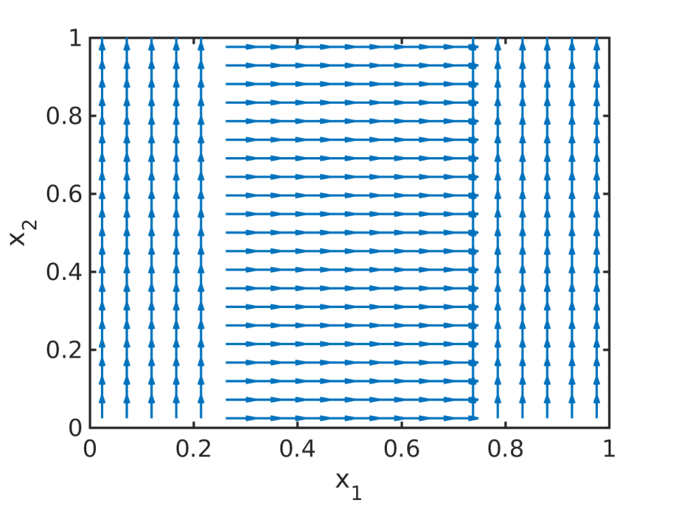
In order to use the particle model (1.1) to simulate fingerprint patterns a realistic tensor field is needed. It is well known that fingerprints are composed of two key directional features known as cores and deltas. Hence, we consider the construction of the tensor fields for these two features first. In [37] Huckemann et al. propose to use quadratic differentials for generating the global fields in a fingerprint image. The local field is then generated by the singular points of the field. A core is the endpoint of a single line (cp. Figure ) and a delta occurs at the junction of three lines (cp. Figure ).
For simplicity we consider the origin () as the only singular point, but the idea can be extended to arbitrary singular points . As outlined in [37] one can model the field near the origin by considering the initial value problem
| (4.1) |
for a smooth, positive function and . For the solution to the differential equation is given by
| (4.2) |
Note that the shape of the solution curves does not change for reparametrizations, provided . By varying the associated solution curves form a delta at the origin () as illustrated in Figure . Hence, we require
for a delta at the origin. Note that where denotes the principal argument of the complex number . Further note that can be regarded as the direction of the smallest stress at if is identified with . As outlined in Section 2 the direction of smallest stress is denoted by the unit vector for implying . Thus, the lines of smallest stress on a domain can be obtained by evaluating for all . Note that and result in the same lines of the stress field.


Similarly, the initial value problem
| (4.3) |
generates a field with a core at the origin. Up to reparameterization the solution is given by
| (4.4) |
and the solution curves are illustrated for different initial conditions in Figure . The condition
has to be satisfied for a core at the origin, implying , and as before result in the same lines. Further note that a delta or a core at any can be obtained by linear transformation. In Figure 5 the tensor field for a delta and a core at the singular point are plotted on the unit square .


4.2. Numerical methods
In this section, we describe the general setting for investigating the long-time behavior of solutions to the particle model (1.1), motivated by [11].
We consider the particle model (1.1) where the forces are of the form (1.2) or (1.3) and investigate the patterns of the corresponding stationary solutions. As in [11] and outlined in Section 2.3 we consider the domain , i.e. the unit square with periodic boundary conditions, and we consider a cutoff of the forces as in (2.8) to make the simulations more efficient.
To solve the particle ODE system (1.1) we apply either the simple explicit Euler scheme or higher order methods such as the Runge-Kutta-Dormand-Prince method, all resulting in very similar simulation results. For the numerical simulations we consider for the size of the time step.
4.3. Numerical study of the Kücken-Champod model
Using the tensor fields introduced in Section 4.1 we consider the interaction model (1.1) with forces of the form (1.3) to simulate fingerprint patterns. Here, the repulsion and attraction forces are of the forms (1.5) and (1.6) with force coefficients (2.3) and (2.4), respectively, and we consider the parameters in (2.5) to make the simulations as close as possible to the model suggested by Kücken and Champod in [42]. It is well known that fingerprints develop during pregnancy and stay the same afterwards provided no fingerprint alterations occur. In order to simulate biologically meaningful fingerprints we aim to model fingerprint patterns as stationary solution to the particle model (1.1). Based on the analysis of steady states in Section 3 it is possible to obtain stationary patterns consisting of multiple roughly parallel ridges along the lines of smallest stress. However, the force coefficients need to be chosen appropriately so that the resulting patterns are also stable. For the simulations in Figure 6 we consider the tensor field for the delta constructed in Section 4.1 and depicted in Figure .


One can clearly see in Figure 6 that the particles are aligned along the lines of smallest stress initially, but the patterns dissolve over time and the simulation results have little similarity with fingerprint patterns over large time intervals. Besides, the patterns are clearly no stable steady states in Figure 6. Hence, the question arises why the patterns simplify so much over time for non-homogeneous tensor fields in contrast to the stationary patterns arising for spatially homogeneous tensor fields, cf. [11], and how this can be prohibited.
To study the long-time behaviour of the numerical solution, it is desirable to have efficient numerical simulations and of course efficient simulations are also necessary to to simulate fingerprints based on cell interactions in practice. In Section 2.3 we introduced a cutoff radius for the forces, given by (2.8), in order to deal with the periodic boundary conditions. Since the forces in the Kücken-Champod model (1.1) decrease exponentially, the interaction force between two particles is very small if their distance is sufficiently large. This is also illustrated in Figure for the parameters in (2.5). Hence, defining the cutoff radius as changes the values of the forces only slightly, but it allows us to compute the numerical solution to the Kücken-Champod model (1.1) by using cell lists [1]. The idea of cell lists is to subdivide the simulation domain into cells with edge lengths greater than or equal to the cutoff radius of the interaction forces. All particles are sorted into these cells and only particles in the same or neighbouring cells have to be considered for interactions. This results in significantly faster simulations since we only have to consider those particle pairs with relevant sizes of the interaction forces. Note that the cutoff radius has an impact on the number of lines that occur in the solution as shown in Figure 7 in comparison to a cutoff radius of in Figure 6. In particular the cutoff radius should not be chosen to small because this prevents the accumulation of particles.


Cutoff radius 0.02


Cutoff radius 0.04


Cutoff radius 0.06
The simulation results for the Kücken-Champod model (1.1) in Figures 6 and 7 illustrate that the particles align in roughly parallel lines along the lines of smallest stress initially, but the number of roughly parallel lines decreases as time goes on. In particular, the complex patterns that occur initially are not stationary. We can expect a similar behavior (i.e. initial alignment along the lines of smallest stress of the stress tensor field and subsequent accumulation) of the numerical solution if the parameters in the coefficient functions of the repulsion and attraction force in (2.3) and (2.4) are slightly changed provided they are repulsive along the lines of smallest stress, as well as short-range repulsive and long-range attractive along the lines of largest stress. Denoting the directions of smallest and largest stress by and , respectively, the transition of the initial pattern of multiple lines to fewer and fewer lines along suggests that the attraction forces are very strong resulting in an accumulation of the particles. Note that this transition is also observed for the long-time behavior of the numerical solution to the Kücken-Champod model (1.1) for spatially homogeneous tensor fields in [11] where lines merge over time until finally a steady state of equidistant parallel lines is reached.
In Figure 8 we show the numerical solution to (1.1) for a piecewise spatially homogeneous tensor field, randomly uniformly distributed initial data and , resulting in stationary line patterns along the lines of smallest stress . In particular, this tensor field is not smooth. This suggests that smoothness and periodicity are not necessary to obtain stationary solutions aligned along the lines of smallest stress.


The big impact of the choice of the attraction force along the lines of largest stress can be seen by considering Figure 9. Here, we assume that the total force is given by for for the spatially homogeneous tensor field with , and instead of the definition of as the sum of and in (1.3), i.e. we vary the size of the attraction force and consider a radially symmetric force . In Figure 9 the steady states to the interaction mode (1.1) are shown for different factors of the attraction force , where and initial data distributed equiangularly on a circle with center and radius is considered. One can see in Figure 9 that results in a stationary solution spread over the entire domain, while ring patterns arise as increases. The intermediate state, occurring for , is of interest in the sequel, as it is an example of a more complex pattern and in particular not all the particles accumulate on one single ring as for and due to too attractive forces.


The forces considered in Figure 9 and given by along the lines of largest stress are plotted in Figure 10 for different values of . As observed in the stationary states in Figure 10, the force along the lines of largest stress is purely repulsive for , medium- and long-range attractive for , as well as medium-range attractive and long-range repulsive for . In particular, the medium-range attractive forces for are significantly smaller than for larger values of .


5. A new model for simulating fingerprints
Based on the analysis of stationary states in Section 3 as well as the numerical investigation of the Kücken-Champod model in Section 4.3 we propose a new model for simulating the formation of fingerprints based on cell interactions where fingerprints are obtained as stationary states to our model. As a next step we propose a bio-inspired model for the creation of synthetic fingerprint patterns which can not only be used to model the formation of fingerprints as stationary solutions but also allows to adjust the ridge distances of the fingerprint lines.
5.1. Stationary patterns
In this section we investigate how fingerprints can be obtained as stationary solutions to the Kücken-Champod model (1.1) where the coefficients of the repulsive and attractive forces are given by (2.3) and (2.4), respectively.
5.1.1. Adaptation of the forces in the Kücken-Champod model
Repulsive forces along the lines of smallest stress are an excellent choice to guarantee that the particles form patterns along the lines of smallest stress. Hence we can consider the repulsive coefficient function for the force along with the parameter values in (2.5) where the coefficient functions and of the attraction and repulsion force are given by (2.3) and (2.4), respectively.
Short-range repulsion forces along the lines of largest stress prevent collisions of the particles and medium-range attraction forces are necessary to make the particles form aggregates. However, the long-range forces should not be attractive for modeling complex patterns since strong long-range attraction forces prevent the occurrence of multiple roughly parallel lines as stationary solutions. Motivated by the more complex stationary pattern for in Figure 9 and its desired structure of the forces along the lines of largest stress (short-range repulsive, medium-range attractive, long-range repulsive as depicted in Figure 10) we consider the coefficient function along the lines of largest stress for the parameters in (5.2). Hence, the total force is given by (1.3) where the repulsion force is defined as (2.3) and the attraction force with coefficient function (2.4) has the new form
| (5.1) |
where we set and we consider the parameter values in (5.2).
In Figures 11, 12 and 13 the numerical solutions for the repulsive force (1.5), the attractive force (5.1) and different realistic tensor fields are illustrated. The tensor fields in Figure 11 are given by a delta and a core, respectively, introduced in Section 4.1, while we consider a combination of deltas and cores for the tensor fields in Figures 12 and 13. As desired the particles align in roughly parallel lines along the vector field and because of long-range repulsion forces these nice patterns are not destroyed over time. Further note that the numerical solution in Figures 11, 12 and 13 is shown for very large times so that it can be regarded as stationary. In particular, this implies that the adapted forces can be used to simulate fingerprint pattern and more generally any complex patterns is in principal preserved over time.


Delta


Core


Example 1


Example 2


Example 3
After this adaptation of the forces it is desirable to use the original definition of the forces (1.3) with repulsion and attraction force given by (1.5) and (1.6), respectively, instead of an attraction force of the form (5.1). Along the attraction force (5.1) can be regarded as where is the attraction force along in the original definition of the attraction force in (1.6). Note that the parameter in the definition of the attractive force coefficient in (2.4) is a multiplicative constant. Hence, we multiply the original value of in (2.5) by , resulting in
| (5.2) | ||||
and consider the original definition of the forces in (1.3), (1.5) and (1.6). The forces along the lines of smallest and largest stress are plotted for the parameters in (5.2) in Figure . Note that they are of the same form as the adapted forces (1.3), (1.5) and (5.1) for the original parameter values (5.2), shown in Figure . Because of the same structure of the forces we can expect similar simulation results. In Figure 15 the numerical solution is shown for two examples, a delta, as well as a combination of a core and a delta. One can clearly see that the particles align along the lines of smallest stress and the resulting patterns are preserved over time. Similarly, one can obtain any complex pattern as stationary solution to the Kücken-Champod model (1.1) by adapting the underlying tensor field. In particular, this implies that the Kücken-Champod model (1.1) with forces defined by (1.3), (1.5) and (1.6) for the parameters in (5.2) can be used to simulate fingerprint patterns which are in principal preserved over time.


Example 4


Example 5
The long-time behavior of the numerical solutions to the Kücken-Champod model (1.1) with model parameters (5.2) is investigated in Figure 16 where the numerical solution at large times is illustrated for the tensor field in Example 5 in Figure 15. Note that the pattern changes only slightly over large time intervals, demonstrating that these patterns are close to being stationary.


5.1.2. Pattern formation based on tensor fields from real fingerprints
In this section, we investigate how to simulate fingerprint patterns based on realistic tensor fields. As proposed in [42] the tensor field is constructed based on real fingerprint data. The tensor field is estimated by a combination of the line sensor method [33] and a gradient based method as described in [34, Section 2.1].

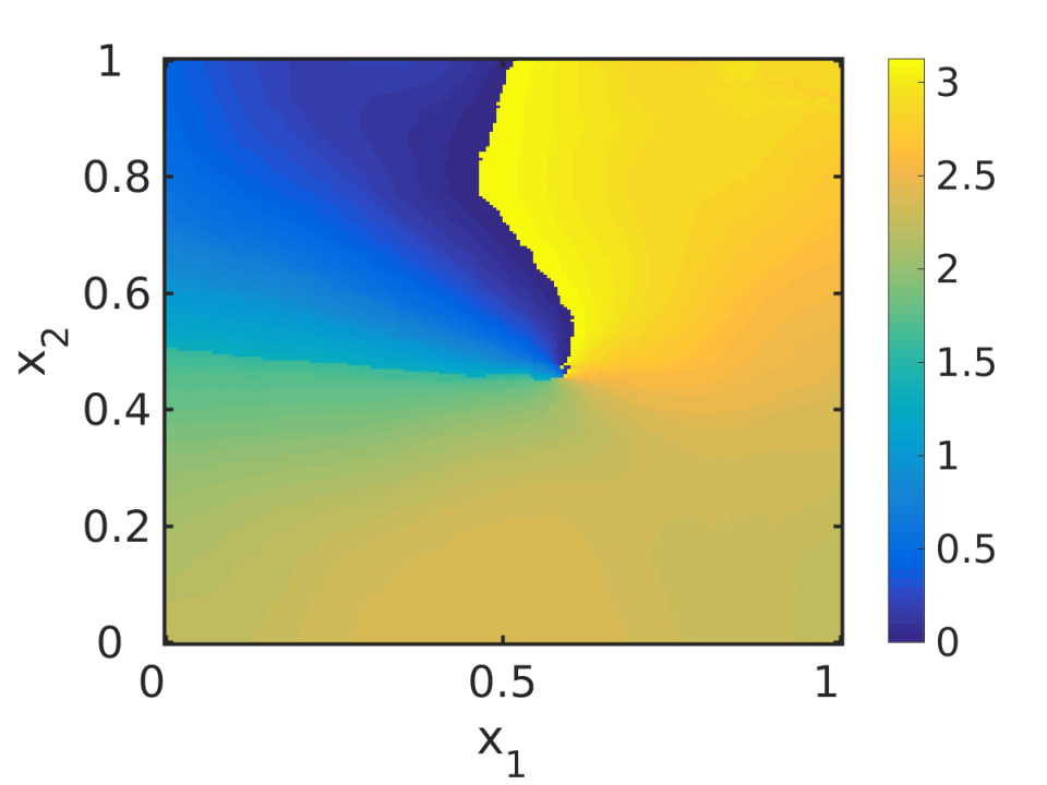

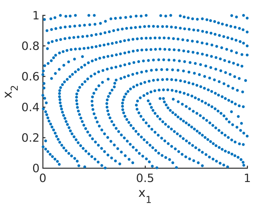
Given some real fingerprint data the aim is to construct the vector field for all as the tangents to the given fingerprint lines. This is based on the idea that the lines of smallest stress are given by and the solution to the interaction model (1.1) aligns along . Let denote the angle between the vertical axis and the direction of lines of smallest stress at location , then it is sufficient to consider the principal arguments only. Note that for any and any given we can reconstruct as since are defined to be unit vectors. In Figure 17 fingerprint data, the estimated arguments for constructing the tensor field and the lines of smallest stress of the tensor field are shown. Note that the lines of smallest stress of the tensor field and the fingerprint lines in the real fingerprint image coincide.
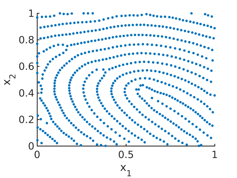
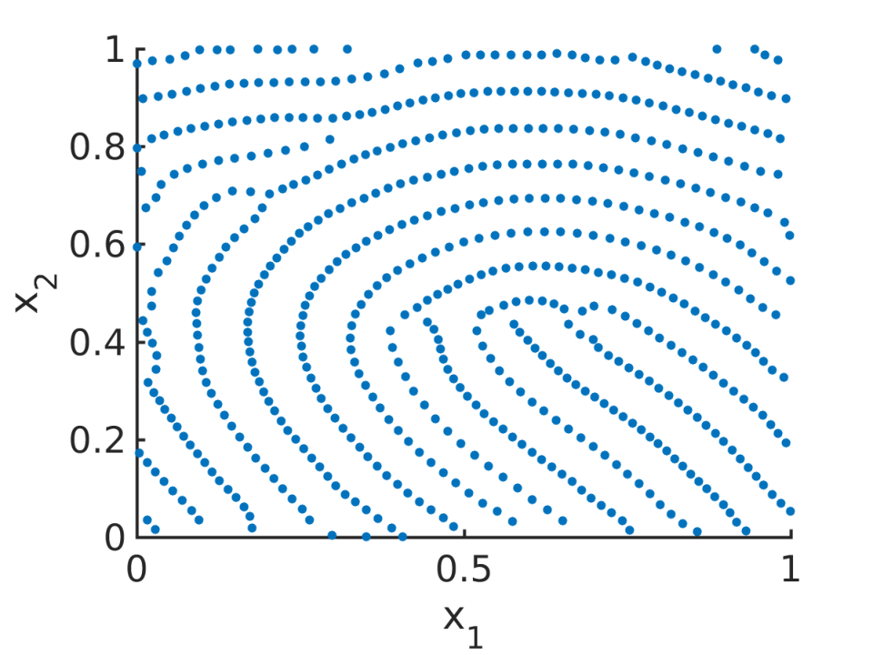
Considering the tensor field shown in Figure 17 the associated numerical solution is plotted for two realizations of uniformly distributed initial data in Figure 18. One can clearly see that the particles align along the lines of smallest stress . Besides, Figure 18 illustrates that we obtain similar, but not exactly the same patterns for different realisations of random uniformly distributed initial data. This is consistent with the well-known fact that everyone has unique fingerprints and even the fingerprints of twins can be distinguished even if the general patterns may seem to be quite similar at first glance [23].
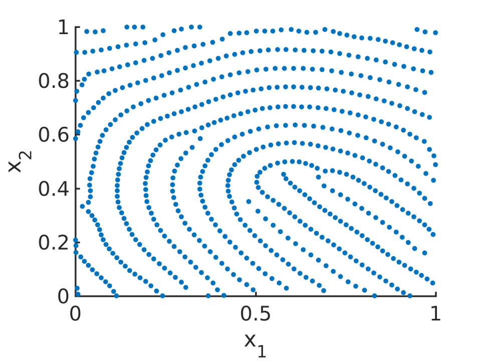
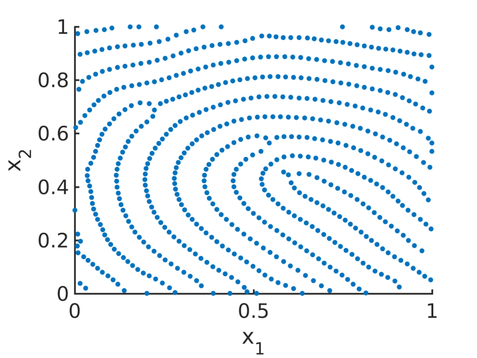
Example 6
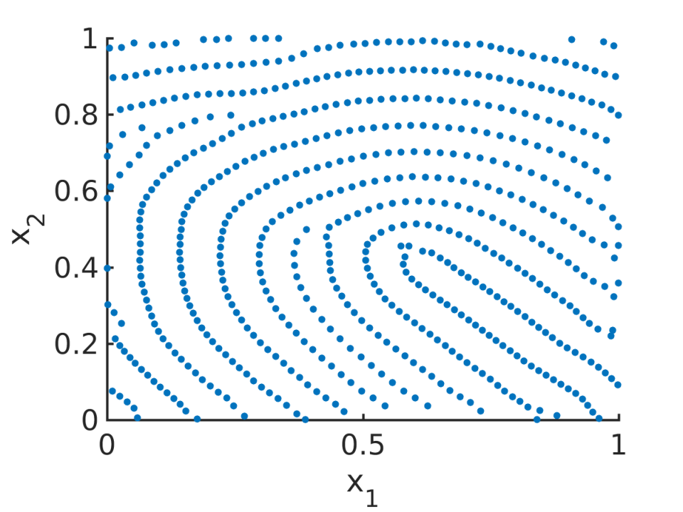
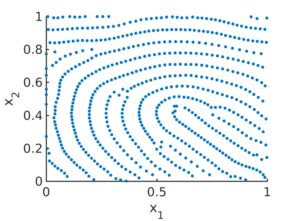
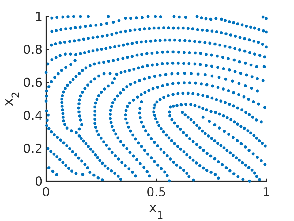
Example 7
To quantify the distance to the steady state we consider the change of the positions of the particles in successive time steps, given by
| (5.3) |
In Figure 19 we show the error between successive time steps for the numerical solution in Example 6 in Figure 18 to the Kücken-Champod model (1.1). After a sharp initial decrease the total change in positions of the particles is approximately , i.e. the movement of the particles is roughly between time steps.

5.1.3. Interpretation of the pattern formation
In the simulations for spatially homogeneous tensor fields in [11] as well as for realistic tensor fields in Figures 11, 12, 13, 15, 16, 18 one can see bifurcations in the solution pattern for certain time steps. More precisely, there exist points where two roughly parallel lines merge with a third roughly parallel line from the other side. These patterns are in the form of the letter ‘Y’. The evolution of one of these bifurcations is shown in Figure 20 for the underlying tensor field in Example 6 in Figure 18. Note that all these lines are aligned along the lines of smallest stress of the tensor field and these bifurcations move towards the two neighboring lines over time. This behavior can be explained by attraction forces along the lines of largest stress over medium range distances, i.e. as soon as the distance between the particles along the lines of largest stress is small enough they attract each other. In particular, the particles close to the bifurcation on the two neighboring lines are the first ones to ‘feel’ the attraction force along and the two roughly parallel lines start merging close to the bifurcation. Hence, the single line on the other side of the bifurcation gets longer over time and the bifurcation moves towards the two parallel lines. While the two roughly parallel lines get shorter over time until they are finally completely merged, resulting in one single line. Since the movement of the particles is mainly along there is a different particle at the bifurcation at each time step. While the particles on the line in the middle roughly remain at the same position apart from realigning along the lines of smallest stress . This realignment along is due to the additional number of particles which are aligned along one single line after the merging, as well as due to the repulsive forces along spreading the particles to make use of the space along and to avoid high particles densities after merging.

5.2. Variable ridge distances
5.2.1. Motivation for a new model
The results in Section 5.1.2 illustrate that it is possible to simulate realistic fingerprints with the Kücken-Champod model (1.1). As seen in the figures, there is some variability in ridge distances and in view of realistic biometric applications, it is of great interest to control them. Note that the total force in (1.3), given by the sum of repulsion and attraction force and of the form (1.5) and (1.6), respectively, can be rewritten as
| (5.4) |
by using the definition of the tensor field in (1.4) and the definition of the distance vector . The coefficient functions of the repulsion and attraction forces (2.3) and (2.4), respectively, are plotted along and for the parameters in (5.2) in Figure . In particular, this motivates us to consider interaction forces of the form (1.2).
We are interested in rescaling the forces now to vary the distances between the fingerprint lines, i.e. we consider where is the rescaling factor. For we recover the same solution patterns as in Section 5.1.2, while the distances between the fingerprint lines become larger for and smaller for . Note that the force coefficient along is repulsive over long distances. For , the case that has been considered so far, this is fine for the given parameters in (5.2). For , however, the scaling results in repulsive interaction forces along for particles with shorter distances between each other. Besides, short-range forces have a stronger impact on the interactions. Hence, these short-range repulsive interaction forces prevent the accumulation of particles along , resulting in several clusters. Note that the forces along are purely repulsive so that rescaling by any does not change the nature of the forces.
In order to prevent this behavior and to obtain an interaction model that can be used for different rescalings, the forces need to be changed slightly so that we have very small attractive forces along for . This does not influence the pattern formation for , but for rescaling by we can obtain the desired line patterns with smaller distances between each other. In order to achieve this, we consider a straight-forward approach first. We consider two cutoffs and and define the adapted force piece-wise such that for the force is of the form (5.4) as before while for we consider an attraction force tending to zero as . To obtain a continuous force we consider a linear interpolation of the force on . Setting
we consider the force coefficients and for interaction forces of the form (1.2) where the force coefficients are defined as
| (5.5) | ||||
and
| (5.6) |
Here, we consider the parameter values and the parameters in the force coefficients (2.3), (2.4) are given by (5.2). The force coefficient along for is obtained by multiplying the original force along by . This is based on the fact that the force coefficient is repulsive for large distances along for the parameters in (5.2). In Figure 21 the force coefficients and in (5.5) and (5.6), respectively, are shown. In particular, the piecewise definition of only has a small influence of the form. In Figure 22, the stationary solution to the particle model (1.1) for interaction forces of the form (1.2), force coefficients (5.5), (5.6), parameter values (5.2), the underlying tensor field in Figure 17 and different rescaling factors is shown and one can clearly see that leads to smaller ridge distances whereas results in larger ridge distances. In particular, the interaction model (1.1) with interaction forces of the form (1.2) and force coefficients in (5.5) and (5.6) can be used to simulate fingerprints with variable ridge distances. Due to the smaller distances between the fingerprint lines for this leads to a larger number of fingerprint lines on the given domain. Due to this increased number of lines it is desirable to run simulations with larger numbers of particles. However, particle simulations can only be applied efficiently as long as the total particle number is not too large. In order to solve this remedy one can introduce the density associated with the particle positions and consider the associated macroscopic model
| (5.7) | ||||
In future work, advanced numerical methods for solving the macroscopic model (5.7) with anisotropic interaction forces could be developed for simulating fingerprint patterns.


5.2.2. A bio-inspired model for simulating stationary fingerprints with variable ridge distances
In this section, we consider interaction forces of the form (1.2) as before with the aim of simulating fingerprints with variable ridge distances based on a bio-inspired approach. The coefficient functions and in (5.5) and (5.6), respectively, are defined piecewise and it is desirable to obtain a closed form for the coefficient functions. As before we consider exponentially decaying forces describing that short-range interactions between the particles are much stronger than long-range interactions. Since the forces are repulsive and attractive on different regimes, this interplay between repulsion and attraction forces can be regarded as oscillations. Motivated by this, we model the force coefficients and in (1.2) as solutions to a damped harmonic oscillator. Note that harmonic oscillators are a common modeling approach in cell biology and the force coefficients are given by (2.6) and are shown in Figure 23 for the parameters in (2.7) in comparison with the piecewise defined force coefficients for the parameters in (5.2). Note that the parameters (2.7) are chosen in such a way that the coefficient functions of the harmonic oscillator approximate the piecewise defined coefficient functions in (5.5),(5.6), respectively. In Figure 24 the stationary patterns to (1.1) for different rescaling factors are shown. As expected the larger the value of the smaller the distances between the fingerprint lines and the more lines occur.


5.2.3. Whole fingerprint simulations
In Figure 25 we construct tensor fields from real fingerprint data based on the methods discussed in Section 5.1.2. We consider a whole fingerprint image shown in Figure and determine the underlying tensor field by estimating the arguments for every . Since we consider the domain we extend the tensor field via extrapolation from the original fingerprint image in Figure , based on [33]. In Figures and the arguments are shown and the arguments are overlayed by the mask of the original fingerprint in black in Figure . Since is a unit vector and hence uniquely determined by its argument we reconstruct the lines of smallest stress as in Figures and , and overlay the direction field by the original fingerprint image in black in Figure . We run simulations for these realistic tensor fields using our new bio-inspired model (1.1) with interaction forces of the form (1.2), force coefficients (2.6) inspired from harmonic oscillators and parameter values in (2.7) for randomly uniformly distributed initial data and particles. Note that the patterns are preserved over time.


Acknowledgments
BD has been supported by the Leverhulme Trust research project grant ‘Novel discretisations for higher-order nonlinear PDE’ (RPG-2015-69). SH acknowledges support from the Niedersachsen Vorab of the Volkswagen Foundation and the DFG Graduate Research School 2088. LMK has been supported by the UK Engineering and Physical Sciences Research Council (EPSRC) grant EP/L016516/1. CBS acknowledges support from Leverhulme Trust project on ‘Breaking the non-convexity barrier’, EPSRC grant Nr. EP/M00483X/1, the EPSRC Centre Nr. EP/N014588/1 and the Cantab Capital Institute for the Mathematics of Information.
References
- [1] M. Allen and D. Tildesley. Computer Simulation of Liquids. Oxford University Press, 1989.
- [2] L. A. Ambrosio, N. Gigli, and G. Savaré. Gradient flows in metric spaces and in the space of probability measures. Lectures in Mathematics. Birkhäuser, 2005.
- [3] D. Balagué, J. A. Carrillo, T. Laurent, and G. Raoul. Dimensionality of local minimizers of the interaction energy. Archive for Rational Mechanics and Analysis, 209(3):1055–1088, 2013.
- [4] D. Balagué, J. A. Carrillo, T. Laurent, and G. Raoul. Nonlocal interactions by repulsive-attractive potentials: radial ins/stability. Physica D: Nonlinear Phenomena, 260:5–25, 2013.
- [5] D. Balagué, J. A. Carrillo, and Y. Yao. Confinement for repulsive-attractive kernels. Disc. Cont. Dyn. Sys.-B, 19:1227–1248, 2014.
- [6] N. Bellomo and J. Soler. On the mathematical theory of the dynamics of swarms viewed as complex systems. Math. Models Methods Appl. Sci., 22(1), 2012.
- [7] A. J. Bernoff and C. M. Topaz. A primer of swarm equilibria. SIAM J. Appl. Dyn. Syst., 10:212–250, 2011.
- [8] A. L. Bertozzi, J. A. Carrillo, and T. Laurent. Blow-up in multidimensional aggregation equations with mildly singular interaction kernels. Nonlinearity, 22(3):683, 2009.
- [9] A. L. Bertozzi, T. Laurent, and F. Léger. Aggregation and spreading via the newtonian potential: The dynamics of patch solutions. Mathematical Models and Methods in Applied Sciences, 22(supp01):1140005, 2012.
- [10] M. Bodnar and J. J. L. Velazquez. Derivation of macroscopic equations for individual cell-based models: a formal approach. Mathematical Methods in the Applied Sciences, 28(15):1757–1779, 2005.
- [11] M. Burger, B. Düring, L. M. Kreusser, P. A. Markowich, and C.-B. Schönlieb. Pattern formation of a nonlocal, anisotropic interaction model. Math. Models Methods Appl. Sci., 2018. (arXiv:1610.08108).
- [12] J. A. Cañizo, J. A. Carrillo, and Francesco S. Patacchini. Existence of compactly supported global minimisers for the interaction energy. Archive for Rational Mechanics and Analysis, 217(3):1197–1217, 2015.
- [13] R. Cappelli, A. Erol, D. Maio, and D. Maltoni. Synthetic fingerprint-image generation. In Proc. 15th Int. Conf. Pattern Recogn. (ICPR), pages 3–7, Barcelona, Spain, September 2000.
- [14] J. A. Carrillo, M. G. Delgadino, and A. Mellet. Regularity of local minimizers of the interaction energy via obstacle problems. Communications in Mathematical Physics, 343(3):747–781, 2016.
- [15] J. A. Carrillo, M. Di Francesco, A. Figalli, T. Laurent, and D. Slepčev. Global-in-time weak measure solutions and finite-time aggregation for nonlocal interaction equations. Duke Math. J., 156(2):229–271, 02 2011.
- [16] J. A. Carrillo, B. Düring, L. M. Kreusser, and C.-B. Schönlieb. Stability analysis of line patterns of an anisotropic interaction model. in preparation.
- [17] J. A. Carrillo, L. C. F. Ferreira, and J. C. Precioso. A mass-transportation approach to a one dimensional fluid mechanics model with nonlocal velocity. Advances in Mathematics, 231(1):306 – 327, 2012.
- [18] J. A. Carrillo, M. Fornasier, J. Rosado, and G. Toscani. Asymptotic flocking dynamics for the kinetic cucker–smale model. SIAM Journal on Mathematical Analysis, 42(1):218–236, 2010.
- [19] J. A. Carrillo, M. Di Francesco, A. Figalli, T. Laurent, and D. Slepčev. Confinement in nonlocal interaction equations. Nonlinear Analysis: Theory, Methods and Applications, 75(2):550 – 558, 2012.
- [20] J. A. Carrillo, F. James, F. Lagoutière, and N. Vauchelet. The filippov characteristic flow for the aggregation equation with mildly singular potentials. Journal of Differential Equations, 260(1):304 – 338, 2016.
- [21] J. A. Carrillo, R. J. McCann, and C. Villani. Kinetic equilibration rates for granular media and related equations: entropy dissipation and mass transportation estimates. Revista Matematica Iberoamericana, 19:971–1018, 2003.
- [22] J. A. Carrillo, R. J. McCann, and C. Villani. Contractions in the 2-wasserstein length space and thermalization of granular media. Archive for Rational Mechanics and Analysis, 179(2):217–263, 2006.
- [23] C. Champod, C. J. Lennard, P. Margot, and M. Stoilovic. Fingerprints and Other Ridge Skin Impressions, Second Edition. International Forensic Science and Investigation. CRC Press, 2016.
- [24] D. Dell and B. Munger. The early embryogenesis of papillary sweat duct ridges in primate glabrous skin: the dermatotopic map of cutaneous mechanoreceptors and dermatoglyphics. J. Comp. Neurol., 244:511–532, 1986.
- [25] J. H. M. Evers, R. C. Fetecau, and L. Ryzhik. Anisotropic interactions in a first-order aggregation model. Nonlinearity, 28(8):2847–2871, 2015.
- [26] J. H. M. Evers, R. C. Fetecau, and W. Sun. Small inertia regularization of an anisotropic aggregation model. Math. Models Methods Appl. Sci., 27(10):1795–1842, 2017.
- [27] K. Fellner and G. Raoul. Stable stationary states of non-local interaction equations. Mathematical Models and Methods in Applied Sciences, 20(12):2267–2291, 2010.
- [28] K. Fellner and G. Raoul. Stability of stationary states of non-local equations with singular interaction potentials. Mathematical and Computer Modelling, 53(7–8):1436 – 1450, 2011. Mathematical Methods and Modelling of Biophysical Phenomena.
- [29] R. C. Fetecau and W. Sun. First-order aggregation models and zero inertia limits. Journal of Differential Equations, 259(11):6774–6802, 2015.
- [30] M. Fornasier, J. Haskovec, and G. Toscani. Fluid dynamic description of flocking via the Povzner–Boltzmann equation. Physica D: Nonlinear Phenomena, 240(1):21 – 31, 2011.
- [31] C. Gottschlich. Curved-region-based ridge frequency estimation and curved Gabor filters for fingerprint image enhancement. IEEE Transactions on Image Processing, 21(4):2220–2227, April 2012.
- [32] C. Gottschlich and S. Huckemann. Separating the real from the synthetic: Minutiae histograms as fingerprints of fingerprints. IET Biometrics, 3(4):291–301, December 2014.
- [33] C. Gottschlich, P. Mihăilescu, and A. Munk. Robust orientation field estimation and extrapolation using semilocal line sensors. IEEE Transactions on Information Forensics and Security, 4(4):802–811, December 2009.
- [34] C. Gottschlich and C.-B. Schönlieb. Oriented diffusion filtering for enhancing low-quality fingerprint images. IET Biometrics, 1(2):105–113, June 2012.
- [35] S.-Y. Ha and J.-G. Liu. A simple proof of the cucker-smale flocking dynamics and mean-field limit. Comm. Math. Sci., 7:297–325, 2009.
- [36] S.-Y. Ha and E. Tadmor. From particle to kinetic and hydrodynamic descriptions of flocking. Kinet. Relat. Models, 1:415–435, 2008.
- [37] S. Huckemann, T. Hotz, and A. Munk. Global models for the orientation field of fingerprints: An approach based on quadratic differentials. IEEE Transactions on Pattern Analysis and Machine Intelligence, 30:1507–1519, 2008.
- [38] C. Imdahl, S. Huckemann, and C. Gottschlich. Towards generating realistic synthetic fingerprint images. In Proc. ISPA, pages 78–82, Zagreb, Croatia, September 2015.
- [39] M. K. Irmak. Multifunctional merkel cells: their roles in electromagnetic reception, fingerprint formation, reiki, epigenetic inheritance and hair form. Med. Hypotheses, 75:162–168, 2010.
- [40] T. K. Karper, A. Mellet, and K. Trivisa. Hydrodynamic limit of the kinetic cucker–smale flocking model. Mathematical Models and Methods in Applied Sciences, 25(01):131–163, 2015.
- [41] D.-K. Kim and K. A. Holbrook. The appearance, density, and distribution of merkel cells in human embryonic and fetal skin: Their relation to sweat gland and hair follicle development. Journal of Investigative Dermatology, 104(3):411 – 416, 1995.
- [42] M. Kücken and C. Champod. Merkel cells and the individuality of friction ridge skin. Journal of Theoretical Biology, 317:229 – 237, 2013.
- [43] H. Li and G. Toscani. Long-time asymptotics of kinetic models of granular flows. Archive for Rational Mechanics and Analysis, 172(3):407–428, 2004.
- [44] S. Moore and B. Munger. The early ontogeny of the afferent nerves and papillary ridges in human digital glabrous skin. Dev. Brain. Res., 48:119–141, 1989.
- [45] K. Morohunfola, T. Jones, and B. Munger. The differentiation of the skin and its appendages - normal development of the papillary ridges. Anat. Rec., 232:587–598, 1992.
- [46] G. Raoul. Non-local interaction equations: Stationary states and stability analysis. Differential Integral Equations, 25:417–440, 2012.
- [47] C. Villani. Topics in optimal transportation. Graduate studies in mathematics. American Mathematical Society, cop., Providence (R.I.), 2003.
- [48] J. H. von Brecht and D. Uminsky. On soccer balls and linearized inverse statistical mechanics. Journal of Nonlinear Science, 22(6):935–959, 2012.
- [49] J. H. von Brecht, D. Uminsky, T. Kolokolnikov, and A. L. Bertozzi. Predicting pattern formation in particle interactions. Mathematical Models and Methods in Applied Sciences, 22(supp01):1140002, 2012.
- [50] K. Wertheim. Embryology and morphology of friction ridge skin. In Fingerprint Sourcebook, chapter 3. National Institute of Justice (NIJ), USA, 2011.