Impact of rainfall on Aedes aegypti populations

L. D. Valdez Affiliation: Facultad de Matemática, Astronomía, Física y Computación, Universidad Nacional de Córdoba, Instituto de Física Enrique Gaviola, CONICET, Ciudad Universitaria, 5000 Córdoba, Argentina G. J. Sibona Affiliation: Facultad de Matemática, Astronomía, Física y Computación, Universidad Nacional de Córdoba, Instituto de Física Enrique Gaviola, CONICET, Ciudad Universitaria, 5000 Córdoba, Argentina C. A. Condat Affiliation: Facultad de Matemática, Astronomía, Física y Computación, Universidad Nacional de Córdoba, Instituto de Física Enrique Gaviola, CONICET, Ciudad Universitaria, 5000 Córdoba, Argentina

Abstract

Aedes aegypti is the main vector of multiple diseases, such as Dengue, Zika, and Chikungunya. Due to modifications in weather patterns, its geographical range is continuously evolving. Temperature is a key factor for its expansion into regions with cool winters, but rainfall can also have a strong impact on the colonization of these regions, since larvae emerging after a rainfall are likely to die at temperatures below $10^{\circ}$ C. As climate change is expected to affect rainfall regimes, with a higher frequency of heavy storms and an increase in drought-affected areas, it is important to understand how different rainfall scenarios may shape Ae. aegypti’s range. We develop a model for the population dynamics of Ae. aegypti, coupled with a rainfall model to study the effect of the temporal distribution of rainfall on mosquito abundance. Using a fracturing process, we then investigate the effect of a higher variability in the daily rainfall. As an example, we show that rainfall distribution is necessary to explain the geographic range of Ae. aegypti in Taiwan, an island characterized by rainy winters in the north and dry winters in the south. We also predict that a higher variability in the rainfall time distribution will decrease the maximum abundance of Ae. aegypti during the summer. An increase in daily rainfall variability will likewise enhance its extinction probability. Finally, we obtain a nonlinear relationship between dry season duration and extinction probability. These findings can have a significant impact on our ability to predict disease outbreaks.

I Introduction

The prevalence areas of both emerging and well-established [1, 2, 3, 4, 5] vector-borne diseases are likely to be substantially modified by climate variations. Being Ae. aegypti the main vector of several important diseases, its ecology is currently the focus of intense research. Since climate is a key determinant of the mosquito habitat [6], climate change is expected to significantly alter its geographic range and put new regions at risk. To predict the future evolution of this range it is necessary to have a clear understanding of how different climatic factors affect Ae. aegypti’s thriving and survival. While temperature governs its reproduction, maturation and mortality rates [7], rainfalls generate breeding grounds for larvae and pupae [8]. At variance with other mosquito species, Ae. aegypti’s eggs are laid above the water surface and hatch only when the water level rises and wets them. The long survival times of its dry eggs endow Ae. aegypti with a competitive advantage over other mosquito species during long periods of drought, but a winter rain may force their hatching and the subsequent larval death. The determination of how climate change may affect the geographical distribution of this mosquito is thus highly nontrivial. In this paper we address the influence of different rainfall regimes on Ae. aegypti.

Aedes aegypti inhabits tropical and subtropical regions worldwide, its geographic range being roughly limited by the $10^{\circ}$ C winter isotherms [9]. The areas close to these isotherms are called “cool margins” [10, 11]. Although the literature describing the reproduction, maturation, and mortality rates, and the dynamics of the mosquito population in warm climates is vast [12, 13, 14, 15], fewer studies have been conducted in the “cool margins”, which often receive cold fronts in winter. Rozeboom [16] studied the survival of Ae. aegypti during the winter in Stillwater, Okla. (USA), where the temperature is often below freezing. This author found that only those Ae. aegypti eggs that were protected from rain and snow became vigorous adults. Later on, Tsuda and Takagi [17] studied the survival of larvae in Nagasaki, Japan, finding that they did not tolerate the low winter temperatures. While Tsuda and Takagi did not perform a direct study with rainfall, they suggested that winter rainfalls could cause mosquito eggs to hatch before spring, and hence the larvae could die due to the low temperatures. Similarly, Chang et al. [18] found in field studies in Taiwan that larval mortality increases rapidly due to cold fronts. Since rainfall may trigger the hatching process, winter rainfalls could impact negatively on Ae. aegypti’s ability to colonize new regions, especially in the “cool margins”. In addition, as climate change is expected not only to increase the temperature but also the frequency of storms and droughts [19], it is important to evaluate how a higher variability in precipitation will affect the dynamics of the mosquito population.

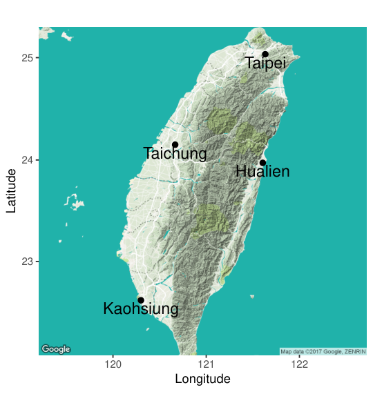
In this work we study the effect of different rainfall regimes on the survival of Ae. aegypti, using Taiwan as an example for our description. This island is an excellent case study. Its average summer temperatures are usually above $20^{\circ}$ C and it receives abundant rainfall throughout its territory [20]. Taiwan has winter isotherms above $10^{\circ}$ C, although northern temperatures are slightly lower than those in the south. Crucially, the rainfall regime in winter is not spatially homogeneous, due to the presence of the Central Mountain Range [21]. For instance, in January Taipei (located in the north) receives an average rainfall of 83mm, whereas in Kaohsiung (located in the south) the average rainfall is 16mm. On the other hand, despite the small surface of Taiwan, entomological studies indicate that the Ae. aegypti population occurs only in the south [22, 23], so we posit that winter rainfall is a determinant for the absence of Ae. aegypti in the north of the country.

We calibrate our model of mosquito populations to reproduce the actual geographical distribution of mosquitoes in four representative Taiwanese cities. Our model correctly predicts that Ae. aegypti should not be present in Taipei, but thrive in Kaohsiung, but it also predicts that, if we reversed the rainfall data for these two cities we would find that this species would become extinct in Kaohsiung but prosper in Taipei. This result provides a strong validation of our working hypothesis. To find out how different rainfall regimes would impact on the mosquito population dynamics, we present a model to generate synthetic rainfall time series. This model is based on a fracturing method [24], which allows us to modify the temporal distribution of rainfall. Using this rainfall model, we find that the four Taiwanese cities have favorable conditions during the summer for the reproduction of Ae. aegypti. In addition, we obtain that, as the variability of rainfall increases, the maximum mosquito abundance $M_{max}$ diminishes. Then, we explore the effect of winter on the survival of Ae. aegypti, obtaining that in all cities except Taipei a decrease in rainfall variability reduces the likelihood of mosquito extinction. Additionally, we analyze how mosquitoes would withstand winter in the four cities if the rate of reproduction changed considering the same rainfall regime, and we find that Kaohsiung is still the most favorable city for these mosquitoes. Finally, we study how the duration of the dry period affects mosquito survival, obtaining a nonlinear relationship between these two variables.

II Models and Results

II.1 The model of mosquito abundance

In this section we introduce a climate-driven abundance model of Ae. aegypti mosquitoes, using four main compartments: eggs ( $E_{T}$ ), larvae (L), pupae (P), and adult mosquitoes (M). In addition, we distinguish between dry ( $E_{D}$ ) and wet eggs ( $E_{W}$ ). The former are those eggs that have not been in contact with water and therefore cannot hatch, while the latter are those that were in contact with water, which we will assume to come only from rainfall. In our model only wet eggs develop into larvae. In Fig. 1 we show a schematic of the transitions between compartments and in Table 1 we present a summary of the parameters of our model that are related with oviposition and rainfall. In the following, we will explain the dependence of the transition rate coefficients with temperature and rainfall.

Figure 1: Schematic representation of the Ae. aegypti evolution through different maturation stages. Mosquito compartments are: dry eggs (

E_{D}

), wet eggs (

E_{w}

), larvae (L), pupae (P), and adult mosquitoes (M). Thin arrows symbolize a waiting time transition which follows an exponential function, whereas the thick arrow represents a delta waiting time distribution from dry eggs to wet eggs (see Sec. “Rainfall and wet eggs”). Transition, maturation, and mortality rates are described in the Appendix.

Table 1: Variables and parameters related with oviposition and rainfall

Quantity	Definition
$\beta$	birth rate of mosquitoes in optimal conditions (days^-1)
$\theta$	effect of the temperature on the mosquito birth rate
$K_{L}$	carrying capacity
$H_{max}$	maximum daily amount of accumulated rainwater [mm]
$H$	accumulated amount of rainwater [mm]
$R$	daily rainfall [mm]
$Evap$	daily evapotranspiration [mm]
$k$	constant of the Ivanov model [mm/^∘C²] (see Eq. 6)
$T$	average daily temperature [^∘C]
$Hum$	daily relative humidity

II.1.1 Survival of Ae. aegypti at low temperatures

Contrary to other Aedes species, such as Ae. albopictus or Ae. albifasciatus, which survive freezing temperatures [25, 26, 27], different studies suggest that Ae. aegypti eggs only survive a few hours at low temperatures. For example, Hatchett [28] found that only $40\%$ of Ae. aegypti eggs could hatch after they were immersed in water and exposed to 1^∘C for 24hs; Chang et al. [18] found that the larval mortality rate increases rapidly when the minimum temperature is below about 10^∘C. On the other hand, historical global collections suggest that Ae. aegypti is distributed geographically only in areas with winter isotherms above 10^∘C [9]. Therefore, we will assume in this work that all mosquito compartments that are in contact with water, $i.e.$ wet eggs, larvae, and pupae, lose a 50% of their members at the end of any day whose minimum temperature is below 10^∘C (see Appendix Sec. “Integration of the equations of our model”). Above this threshold, the dependence of the mortality rate with the temperature for each compartment is that given by Barmak et al. [29] (see Appendix Sec. “Mortality rates”).

II.1.2 Rainfall and wet eggs

Ae. aegypti lays its eggs on the inner side of containers above the water line (see Ref. [30]). These eggs are regarded in our model as dry eggs and when they are flooded, for example by rainwater, they usually hatch. Therefore, following the work of Aznar et al. [31], we propose that, if on day $d$ it rains $R$ millimeters, the fraction of dry eggs that become wet eggs is given by the following Hill function,

\displaystyle f(R)=0.8\frac{(R/R_{thres})^{5}}{1+(R/R_{thres})^{5}}.

(1)

Here, $R_{thres}$ is the rainfall threshold and the prefactor $0.8$ stands for the maximum fraction of eggs that may hatch when they are flooded. In this work, we set $R_{thres}=10$ [mm]. This function is applied at the end of day $t=d$ on the dry egg compartment, where $t$ is a continuous variable and $d$ is a non-negative integer (see Appendix Sec. “Integration of the equations of our model”).

II.1.3 Effect of rainfall on the carrying capacity

The persistence of breeding sites is a key factor for the survival of mosquitoes in the aquatic stage. Rainfall creates breeding sites where larvae develop prior to becoming adult mosquitoes, and evaporation tends to shrink these sites. Therefore, we propose that the carrying capacity depends on the amount of available water $H(t)$ , whose variation is defined as follows:

\displaystyle H(t+1)=\left\{\begin{array}[]{ll}0&\;\;\;\;\text{if}\;\;\;\;H(t)+\Delta(t)\leqslant 0\\ H_{max}&\;\;\;\;\text{if}\;\;\;\;H(t)+\Delta(t)\geqslant H_{max}\\ H(t)+\Delta(t)&\;\;\;\;\text{otherwise},\\ \end{array}\right.

where $\Delta(t)=R(t)-Evap(t)$ , $R(t)$ is the amount of rain on day $t$ and $Evap(t)$ is the daily evaporation. Note that $H$ can increase only up to a maximum value $H_{max}$ since we consider that at a higher water level the containers or breeding sites overflow. Besides, following the Ivanov model [32, 33], we propose that the evaporation rate $Evap(t)$ is given by the expression,

\displaystyle Evap(t)=k(25+T(t))^{2}(100-Hum(t)).

(6)

where $T$ is the average temperature and $Hum$ the humidity. Finally, we propose that the carrying capacity is given by:

K_{L}(t)=K_{max}\frac{H(t)}{H_{max}}+1,

(7)

where $K_{max}$ is the maximum carrying capacity and the $1$ is introduced to avoid divergences if $H(t)\to 0$ .

For more details of our model of Ae. aegypti mosquitoes see Appendix Sec. “Transitions rates”. In the following section we will apply our mosquito model to study the case of Taiwan, using the actual rainfall time series.

III Case study: Taiwan

As mentioned in the Introduction, to study how different rainfall regimes impact on the mosquito population it is informative to analyze the case of Taiwan. More specifically, we will apply our model to study mosquito populations in four cities in Taiwan: Taipei (north), Taichung (west), Hualien (east), and Kaohsiung (south). In Figs. S1 (see Appendix Sec. “Weather in Taiwan”) we show their average, minimum, and maximum daily temperatures in the period 2010-2013, and the average monthly precipitation $\mathscr{P}(m)$ in the period 1981-2010. Of these four cities, an established Ae. aegypti population has been found only in Kaohsiung. We investigate the reasons why.

In order to model the actual distribution of Ae. aegypti in these cities, we calibrate a deterministic version of our model to the time series of adult Ae. aegypti abundances per block in Kaohsiung in the period January 2010-December 2012. Namely, we use a Latin hypercube sampling (LHS) method to generate points in a four-dimensional space defined by the vector $(\beta,k,H_{max},K_{max})$ . Additionally, since Taipei, Taichung, and Hualien do not have permanent Ae. aegypti populations, for each point of the LHS method we also obtain the abundance of adult mosquitoes corresponding to each city, computing the mean square distance between them and a null abundance mosquito series. Finally, we select the point of the LHS that minimizes the sum of the mean square distances for the four cities. See Appendix Sec. “Model calibration” for more details of the calibration process. In Table 2 we show the estimated values of the parameters.

Table 2: Estimated values of

(\beta,k,H_{max},K_{max})

using a Latin hypercube sampling.

parameter	values
$\beta$	0.52
$k$	3.9 $10^{-5}$
$H_{max}$	24
$K_{max}$	212

In Fig. 2a we show the actual time series of the abundance of adult mosquitoes [34] and the predictions of our model using the parameters obtained with the calibration process and the actual time series of temperature, rainfall, and humidity of Kaohsiung [20]. Although our model does not reproduce exactly the heights of the actual mosquito abundance, the positions of the peaks are well correlated with the data. We recall that the Aedes populations in the other cities are extinct.

Figure 2: (a) Time series of the number of adult Ae. aegypti mosquitoes obtained from the Kaohsiung data (circles) [34] and the prediction of our model (solid line), using the parameters from Table 2 and the actual time series of temperature, rainfall, and humidity for Kaohsiung in the period January 2010-December 2012 [20]. For the calibration we have re-scaled the actual time series of adult mosquito abundances, so that this abundance is of 100 mosquitoes in the summer. (b) Evolution of the mosquito abundance using the calibrated parameters shown in Table 2 and the actual meteorological data of Kaohsiung and Taipei, but where we swapped the rainfall time series of these two cities. The solid red (dashed black) line corresponds to the case of temperature and humidity of Taipei (Kaohsiung) and the rainfall of Kaohsiung (Taipei).

In order to ascertain if rainfall is indeed responsible for the distribution of Ae. aegypti mosquitoes in Taiwan, we computed the dynamics of mosquito abundances in Kaohsiung and Taipei, but exchanging the actual rainfall time series between these places. As it can be seen from Fig. 2b, in this hypothetical scenario where Taipei has drier winters, it could maintain a sizable population of mosquitoes through the years. On the other hand, if Kaohsiung had rainy winters, Ae. aegypti would become extinct there. These results confirm that our model is effective describing scenarios where rainfall controls the mosquito survival.

In the following sections, we introduce the model to generate synthetic rainfall time series, which will allow us to study how different rain regimes can shape Ae. aegypti’s geographic distribution.

IV Synthetic rainfall time series

In order to study the dynamics of mosquito populations for different rainfall regimes, we will use the method to generate synthetic rainfall time series presented in Ref. [35], which we briefly review next. In this method, we must first specify the total monthly rainfall $\mathscr{P}(m)$ and the monthly number of rainy days $\mathscr{D}(m)$ , where $m$ stands for the month. These variables are often used in regression models to predict the number of mosquitoes, as well as to describe the rainfall regime in meteorological forecasting [36, 37, 38, 39]. The values of $\mathscr{P}(m)$ and $\mathscr{D}(m)$ can either be assigned using the actual averages obtained from meteorological data, or they can be modeled using mathematical functions.

To decide how the monthly rainfall $\mathscr{P}(m)$ for a given month $m$ is distributed on a daily basis, we use a fracturing method which consists in successively decomposing the monthly precipitation $\mathscr{P}(m)$ into the sum of two terms (see Refs. [24, 35]), until $\mathscr{P}(m)$ is the sum of $\mathscr{D}(m)$ terms. Namely, this process begins by decomposing $\mathscr{P}(m)$ into two non-negative terms $X_{1}$ and $X_{2}$ with $\mathscr{P}(m)=X_{1}+X_{2}$ where $X_{1}$ is given by

\displaystyle X_{1}=\mathscr{P}(m)\times\left\{\begin{array}[]{ll}\rho\frac{1-\alpha}{\alpha}&\;\;\text{if}\;\;0\leqslant\rho<\frac{\alpha}{2}\\ \frac{1}{2}+\left(\rho-\frac{1}{2}\right)\frac{\alpha}{1-\alpha}&\;\;\text{if}\;\;\frac{\alpha}{2}\leqslant\rho\leqslant 1-\frac{\alpha}{2}\\ 1-(1-\rho)\frac{1-\alpha}{\alpha}&\;\;\text{if}\;\;1-\frac{\alpha}{2}<\rho\leqslant 1\\ \end{array}\right.

where $\rho$ is a uniform random variable and $\alpha\in[0,1]$ is a parameter that controls the variance of the values of $X_{1}$ . In particular, for $\alpha=0$ , $X_{1}=X_{2}=\mathscr{P}(m)/2$ , while for $\alpha=1$ we obtain $X_{1}=0$ and $X_{2}=\mathscr{P}(m)$ . Therefore, an increasing in the value of $\alpha$ generates a rainfall time series with a higher heterogeneity in the daily amount of precipitation. This step is applied iteratively to each term until the total number of terms is $\mathscr{D}(m)$ . Each of these terms corresponds to a total daily rainfall, which is assigned at random to one day of the month.

Although this method allows us to explore different scenarios of rainfall heterogeneity, it is of interest to determine the value of $\alpha$ that best fits an actual rainfall time series, as a reference value for our analysis. To this end, in Appendix Sec. “Calibration of $\alpha$ ”, we develop a method that computes the value of $\alpha$ that best fits the variance of the daily precipitation for a given period of time (usually, one month).

In Table 3 we show the values of $\alpha$ for a few cities. Notably we obtain that the values are all distributed in a relatively narrow range ( $[0.32;0.46]$ ), suggesting that rainfalls are moderately heterogeneous.

Table 3: Estimated values of

\alpha

for several cities. Meteorological data were obtained from Ref. [40] for the city of Hong Kong, from Ref. [41] for the cities in Australia, and from Ref. [42] for the other cities. In the second column we show the month analyzed, which corresponds to the rainiest month in each city.

Cities (number of years analyzed)	Month analyzed	$\bar{\alpha}$
Sydney, Australia (157 years)	April	0.46
Hong Kong, China (126 years)	June	0.44
Alice Springs, Australia (67 years)	February	0.43
Berlin, Germany (134 years)	July	0.39
Atlanta, USA (88 years)	March	0.39
Happy Valley, Australia (46 years)	March	0.38
Los Angeles, USA (91 years)	February	0.38
London, UK (43 years)	October	0.36
Chapingo, Mexico (44 years)	July	0.32

IV.1 Results with synthetic rainfall time series

In this section we apply the model of synthetic rainfall time series to further analyze the effect of rainfall on the mosquito population in Taiwan. In Fig. 3 we show the maximum peak $M_{max}$ of adult mosquito abundance in the summer of 2011 in Taipei and Kaohsiung; here we use the actual temperature and humidity time series and the synthetic rainfall for various values of $\alpha$ . For simplicity, we use the same value of $\alpha$ for all months. We integrate our mosquito model over a period of one year, setting as initial condition $E_{D}=E_{W}=L=P=M=10$ in May 2011, and we use the average rainfall and the mean number of rainy days per month corresponding to the period 1981-2010 for the synthetic rainfall model. From the figure we observe that the peak of abundance is a decreasing function with the heterogeneity $\alpha$ : since the monthly precipitation is concentrated in fewer days when $\alpha$ increases, the mosquitoes have often a smaller amount of water available to reproduce. Similar plots were obtained for Hualien and Taichung (not shown here).

Figure 3:

M_{max}

as a function of

\alpha

using the actual temperature and humidity data for the period May 2011-April 2012. Light blue region: 90% of the 1000 realizations for the synthetic rainfall using the average rainfall and the mean number of rainy days per month corresponding to the period 1981-2010 (see Appendix “Weather in Taiwan”).

We also observe that the four cities in Taiwan have favorable conditions for mosquito breeding during the summer. An important question is whether the mosquito population that invades an unoccupied area in spring-summer is able to survive the winter season, at least as dried eggs. To test this, we integrate the mosquito abundance equations over the period May 2011- April 2012 for the four cities and compute the Ae. aegypti extinction probability $Prob(\alpha)$ at the end of April 2012 for different rainfall heterogeneity values $\alpha$ . Note that we consider that a mosquito species is extinct if the number of members in each compartment is null. In Fig. 4a we observe that $Prob(\alpha)$ is an increasing function with $\alpha$ for all the cities, which is consistent with a decreasing of $M_{max}$ with $\alpha$ as it was shown in Fig. 3. Additionally, we plot in Fig. 4b the extinction probability for different values of the oviposition rate $\beta$ with $\alpha=0.45$ . In this figure we observe that Kaohsiung is the most favorable city for the establishment of mosquitoes. In turn, we note that the probability $Prob(\beta)$ is vanishingly small for $\beta\gtrsim 0.50\equiv\beta_{c}$ in Kaohsiung, which suggests that, in order to model Ae. aegypti populations in this city with a synthetic rainfall time series, we should use an oviposition rate $\beta$ above $\beta_{c}$ .

Figure 4: Aedes aegypti extinction probabilities in Kaohsiung (circles), Hualien (squares), Taichung (diamonds), and Taipei (triangles) as (a) functions of

\alpha

using the calibrated values of Table 2; and (b) as functions of

\beta

with

\alpha=0.45

. Dotted lines serve as a guide to the eye. The results are averaged over 1000 realizations of the synthetic rainfall model.

On the other hand, although Taichung is the second city with the driest winter, our model predicts that the second most favorable city for Ae. aegypti after Kaohsiung is Hualien, which has slightly warmer winters than Taichung. This suggests that temperature can compensate the negative effect of winter rainfall.

IV.1.1 Why is Ae. aegypti not endemic to Hualien?

It is interesting to further discuss the reasons why Ae. aegypti is not endemic to Hualien. Having a temperature similar to Kaohsiung and total winter precipitations that are about half those in Taipei (see Appendix Sec. “Weather in Taiwan”), Hualien is the second most favorable city for the establishment of Ae. aegypti. From Fig. 4 we note that for $0.50\lesssim\beta\lesssim 0.60$ it would be possible to reproduce the real geographic distribution of Ae. aegypti in Taiwan. However, if the true value of the oviposition rate $\beta$ is slightly greater than 0.6, the fact that there are no mosquitoes in Hualien may be due to variables we did not consider in our model, such as competition with other mosquito species [43] or local predators. In addition, Han and Chuang [44] suggested that Hualien presents the highest amount of fungi concentration in the whole country, due to Asian dust storms. For instance, fungal traps in this city revealed the presence of Periconia and Torula (see Ref. [45]). Notably, a recent study found that similar fungi were the cause of mortality of Ae. aegypti eggs in Chaco, Argentina (see Ref. [46]).

IV.1.2 Extinctions and dry season length

Another relevant aspect of a particular rainfall regime is how the duration of the dry season affects the establishment and survival of Ae.aegypti in a city. To study this effect, we will use a model of synthetic rainfall time series in which the amount of monthly rainfall $\mathscr{P}(m)$ and the number of rainy days $\mathscr{D}(m)$ are given by the following functions,

$\displaystyle\mathscr{P}(m)$	$\displaystyle=$	$\displaystyle(P_{max}-P_{min})\left(\frac{1}{2}+\frac{1}{2}\cos\left(\frac{2\pi}{12}(m-m_{0})\right)\right)^{\gamma}+$	(12)
		$\displaystyle+P_{min},$	(12)
$\displaystyle\mathscr{D}(m)$	$\displaystyle=$	$\displaystyle(D_{max}-D_{min})\left(\frac{1}{2}+\frac{1}{2}\cos\left(\frac{2\pi}{12}(m-m_{0})\right)\right)^{\gamma}+$	(13)
		$\displaystyle+D_{min},$	(13)

where $\gamma\in[0,\infty)$ controls the duration of the dry season (the higher the $\gamma$ , the longer the duration of the dry season); $m_{0}$ is the rainiest month of the year, $P_{max}$ is the total precipitation in the rainiest month (in millimeters), and $P_{min}$ that in the driest month. The variables $D_{max}$ and $D_{min}$ have similar interpretations for the number of rainy days. Note that $\mathscr{P}(m_{0})=P_{max}$ and $\mathscr{D}(m_{0})=D_{max}$ for all values of $\gamma$ . Analogously, $\mathscr{P}(m_{0}-6)=P_{min}$ and $\mathscr{D}(m_{0}-6)=D_{min}$ for all values of $\gamma$ . Here, we set $m_{0}=7$ (July). Since the number of rainy days is an integer number but in Eq. (13) $\mathscr{D}(m)$ is a real number, for each rainfall time series realization we choose the number of rainy days to be [ $\mathscr{D}(m)$ ] and [ $\mathscr{D}(m)$ ]+1 with probabilities $\mathscr{D}(m)$ -[ $\mathscr{D}(m)$ ] and $1-(\mathscr{D}(m)-[\mathscr{D}(m)])$ , respectively (here $[\cdots]$ stands for the integer part).

Figure 5: Effect of the dry period on the extinction probability. Using the model of synthetic rainfall time series, we compute (a) the probability of extinction of mosquitoes for each month in Taipei as a function of

\gamma

for

\alpha=0.45

, and (b) the cumulative probability of extinction of Ae. aegypti in Taipei for different values of

\alpha

and

\gamma

. We compute the cumulative probability of extinction after the second year from the date of the initial condition. Panel (b) also shows the average amount of precipitation in a rainy day

\mathscr{P}(m)/\mathscr{D}(m)

(solid white lines) for

m=2,3,4,5,6

and the rainfall threshold

R_{thres}=10

[mm] (see Eq. (1) and dashed red line). The monthly rainfall distribution and the number of rainy days follow Eqs. (12) and (13). We set:

P_{max}=350

P_{min}=0

D_{max}=15

D_{min}=1

, and

m_{0}=7

. The initial condition is

E_{D}=E_{W}=L=P=M=10

on May 1, 2011 and we model the dynamics of mosquito abundance for four years. Cold colors represent a low probability of extinction (black corresponds to a null probability) and warm colors a probability close to 1. The results are averages obtained over 1000 realizations of rainfall time series.

In Fig. 5a we show the probability of extinction of Ae. aegypti for each month as a function of $\gamma$ , for $\alpha=0.45$ . In Appendix Sec. “Effect of the dry season on Ae.aegypti” we show the same plot for $\alpha=0.10$ and $0.80$ ; in all cases we use the actual temperature and humidity time series of Taipei. We observe that for low values of $\gamma$ , that is to say, when the amount of precipitation is high in almost every month, the extinction occurs in winter. This is consistent with the Tsuda and Takagi’s hypothesis, which states that winter rainfalls could cause eggs to hatch in a period with low temperatures (see the Introduction). As $\gamma$ increases, the maximum probability of extinction moves forward in time: dry periods are longer and more intense. Finally for the highest values of $\gamma$ , the extinction occurs in summer: since the (extremely) dry season lasts almost 11 months, very few viable eggs survive until the (short) wet season; these cannot sustain a mosquito population after a rainfall event. Note that extinctions never occur in the fall.

In Fig. 5b we show the effect of the daily rainfall heterogeneity ( $\alpha$ ) and the duration of the dry season ( $\gamma$ ) on the cumulative probability of extinction of Ae. aegypti in the city of Taipei. Again, we use the actual temperature and humidity time series of Taipei. We obtain, as expected, that for very low values of $\gamma$ mosquitoes become rapidly extinct since rainfalls are abundant throughout the year. It should be noted that the probability of extinction does not depend on the daily rainfall variability ( $\alpha$ ). Therefore, when there is no dry season, the amount of monthly rainfall (in millimeters) is a sufficient predictor for determining the absence of mosquitoes. However, as $\gamma$ increases, we observe that the probability of extinction drops, and hence in this parameter domain we can consider that Taipei resembles Kaohsiung. The dry winter allows a bigger egg population to survive; when they hatch in the rainy season the temperature is already high enough to allow these eggs to prosper. Additionally, in this case the probability of extinction also depends on $\alpha$ . This suggests that in areas with dry winter months but without a permanent Ae. aegypti population, the role of the variability in the daily precipitation as an explanatory variable for these extinction cases should be further explored.

On the other hand, note that as $\gamma$ grows for a fixed value of $\alpha$ , the extinction probability increases and decreases several times. In Fig. 5b we show that local transitions from high to low extinction probabilities take place when the average amount of precipitation in a rainy day on month $m$ , $i.e.$ $\mathscr{P}(m)/\mathscr{D}(m)$ is approximately equal to the rainfall threshold (see Eq. (1)). An extinction may occur, for instance, in a month when rainfalls can flood a certain quantity of eggs but the amount of available water is not enough to sustain a larval population; as $\gamma$ increases this month will become a “dry” month, so the probability of extinction diminishes because fewer eggs hatch under detrimental conditions. Finally, for very high values of $\gamma$ , the extinction probability again increases, which is consistent with the results shown in Fig. 5a for a very dry region.

V Summary

Since Ae. aegypti is expanding its territory, potentially contributing to the spread of diseases such as Dengue, Yellow Fever, Chikungunya and Zika [47, 48, 49] to new areas, it is important to assess how different climatic variables can shape the present and future geographic range of this mosquito. We have developed a model for the Ae. aegypti population that takes into account the susceptibility of its immature stages to winter rains. We hypothesize that locations with cool, rainy winters are inimical to this species and test the model by applying it to four cities in Taiwan, reproducing the observed presence (or absence) of Ae. aegypti. In particular, we find that the reason Ae. aegypti is endemic to Kaohsiung is that it is the city with the lowest precipitation in winter. We also introduce a procedure to generate rainfall time series to explore the effect of different rainfall regimes.

Applying our rainfall model to Taiwan, we find that as the precipitation heterogeneity ( $\alpha$ ) increases, the peak of mosquito abundance during the summer decreases. On the other hand, a reduction in the heterogeneity of daily rainfall decreases the probability of extinction in all the cities, except Taipei. We also obtain that the presence or absence of Ae. aegypti depends on a delicate balance between different climatic variables in the regions near the $10^{\circ}$ C winter isotherms.

Finally, we studied the effect of dry season duration on mosquito survival and found that, as it increases, the survival probability also increases. However, because eggs become gradually nonviable, for very long droughts, the likelihood of extinction rises again.

Given that climate change is likely to make the world wetter, predicting the evolution of the geographical habitat of Ae. aegypti is not easy: while an increase in the temperature should shift its boundaries towards higher latitudes, an increase in the winter rainfall would be detrimental to its enlargement. The model presented here can be useful to address this challenge.

Acknowledgments

This work was supported by SECyT-UNC (projects 103/15 and 313/16) and CONICET (PIP 11220150100644). We also thank Mgter. Laura López for useful discussions.

VI Appendix

VI.1 Weather in Taiwan

Refer to caption — Figure S1: Left panel: Map showing the four cities of Taiwan for which we apply our mosquito model using a synthetic rainfall time series: Taipei, Taichung, Hualien, and Kaohsiung [50]. Center panels: Maximum (black line), average (orange line) and minimum (red line) temperatures for each city in the period 2011-2013. The horizontal dashed line stands for the $10^{\circ}$ C isotherm. Rightmost panels: Average monthly rainfall $\mathscr{P}(m)$ in the period 1981-2010 (bar plots), with $m=1$ for January and $m=12$ for December.

VI.2 Effect of the dry season on Ae.aegypti

Figure S2: Probability of extinction of mosquitoes for each month in Taipei as a function of

\gamma

, using the model of synthetic rainfall time series for two

\alpha

values: 0.10 and 0.80. The monthly rainfall distribution and the number of rainy days follow Eqs. (12) and (13). We chose:

P_{max}=350

P_{min}=0

D_{max}=15

D_{min}=1

, and

m_{0}=7

. The initial condition is

E_{D}=E_{W}=L=P=M=10

on May 1, 2011. We model the dynamics of mosquito abundance for four years. Cold colors represent a low probability of extinction (black corresponds to a null probability) and warm colors a probability close to 1. The results were averaged over 1000 realizations of rainfall time series.

Figure S3: Cumulative probability of extinction of Ae. aegypti in Taipei for different values of

\alpha

and

\gamma

, using the model of synthetic rainfall time series. The monthly rainfall distribution and the number of rainy days follow Eqs. (12) and (13). We chose:

P_{max}=350

P_{min}=0

D_{max}=15

D_{min}=1

, and

m_{0}=7

. The initial condition is

E_{D}=E_{W}=L=P=M=10

on May 1, 2011. We compute the cumulative probability of extinction after one (a), three (b) and four (c) years. The colors have the same meaning as in Fig. 5.

VI.3 Model calibration

For the calibration of our mosquito population model, we use a Latin hypercube sampling method for the parameters $\beta$ , $k$ , $H_{max}$ , and $K_{max}$ , and compute the mean square distance between the predicted abundance of mosquitoes and the actual weekly adult mosquito abundance data of Kaohsiung in the period January 2010 - December 2012 (obtained from Ref. [34]). Note that we re-scaled the actual abundance data, so it is about 100 mosquitoes per block in the summer. We set as initial conditions, $E_{D}=E_{W}=L=P=M=100$ . For the same set of points, we repeat the process for Taipei, Taichung, and Hualien ¹¹ 1 For the calibration in Taipei and Kaohsiung, we integrate our equations over the period January 2010- December 2012. For Hualien and Taichung we adjust our model in the period January 2011- December 2012, since the data of temperature and humidity in 2009 are not available.. In all the cases, we start the integration six months before the time from which we compute the mean square distance, in order to minimize the effect of the initial conditions. Note that we use the actual values of temperature, humidity, and rainfall for the calibration process. Finally, we choose the point ( $\beta$ , $k$ , $H_{max}$ , $K_{max}$ ) that minimizes the sum of the square distances corresponding to all the cities.

VI.4 Integration of the equations of our model

We model a system of compartmental difference-differential equations which we integrate numerically using the Euler method with $\Delta t=0.01$ , where $t$ is given in days. If for any time step the population of a compartment is negative, then we change its value to 0. Since the time series of temperature, humidity and rainfall are on a daily time scale, all the parameters that depend on these variables are considered constant between days $d$ and $d+1$ , i.e. for $t\in[d,d+1)$ , where $d$ is a non-negative integer number. These parameters are calculated using the values of temperature, humidity, and rainfall for that day. In turn, if it rains on day $d$ , then at the end of each rainy day, i.e. when $t=d+1-\Delta t$ , a fraction of dry eggs go wet as it is explained in Sec. “Rainfall and wet eggs”. Similarly, if on day $d$ the minimum temperature is below $10^{\circ}$ C, then at time $t=d+1-\Delta t$ we apply the rules explained in Sec. “Survival of Ae. aegypti at low temperatures”. Finally, to incorporate the fact that we model discrete populations and to be able to explore extinction processes, we will impose that if the population of a compartment is less than 1 at the end of the integration step $t=d-\Delta t$ , then we change its value to 0.

VI.5 Calibration of $\alpha$

In order to compute the value of $\alpha$ that best fits the actual rainfall time series, we propose a procedure based on the distance minimization between the variance of the actual rainfall time series and that of the synthetic one. Namely, we propose the following steps:

1.

We calculate the total precipitation $\mathscr{P}$ (in millimeters) and the number of rainy days $\mathscr{D}$ in a period of time (for instance, 30 days) and the variance of the actual daily rainfall. We exclude non-rainy days from the computation of this variance.
2.

We use the fracturing process for different values of $\alpha\in[0,1]$ using the actual values of the total rainfall and the number of rainy days computed in the previous step. Then we measure the variance of the synthetic rainfall series. This step is repeated $10^{5}$ times for each value of $\alpha$ .
3.

We choose the value of $\alpha$ that minimizes the distance between the average variance of the synthetic rainfall and the variance of the actual rainfall time series.

To ascertain if this procedure allows us to re-obtain a preset value of $\alpha$ for a synthetic rainfall time series, we generate these series for different values of $\alpha$ and then we apply the method described above. In Table S1 we show that, although our method slightly underestimates the values of $\alpha$ , the new values are close enough to the preset ones to confirm the consistency of the procedure.

Table S1: Estimated values of

\alpha

for various synthetic rainfall time series. We constructed 100 of these series for each preset value of

\alpha

using a total precipitation of

\mathscr{P}=200

and

\mathscr{D}=10

rainy days in a period of 30 days.

$\alpha$ (preset value)	$\bar{\alpha}$ (estimated value)
0.2	0.16
0.3	0.27
0.4	0.35
0.45	0.42
0.5	0.45
0.6	0.58

VI.6 Transition rates

VI.6.1 The impact of mean daily temperature on oviposition

We propose that the number of dry eggs laid per unit time is proportional to: 1) the number of adult mosquitoes, 2) the oviposition rate $\beta$ in optimal conditions of temperature, and 3) a factor $\theta\in[0,1]$ , which stands for the effect of temperature on oviposition. In this work, $\theta$ is given by

\displaystyle\theta(t)=\left\{\begin{array}[]{ll}0.1137(-5.4+1.8T-0.2124T^{2}+0.01015T^{3}-0.0001515T^{4})&\;\;\;\;\text{if}\;\;\;\;11.7<T(t)<37.2\\ 0&\;\;\;\;\text{otherwise},\end{array}\right.

Here the relation between $\theta$ and the mean daily temperature $T$ was obtained by Yang et al. on the basis of temperature laboratory experiments (see Refs. [51, 52]), and the prefactor 0.1137 normalizes $\theta$ .

VI.6.2 Maturation rates

In table S2 we define the maturation rates $m_{X}$ (where $X=E$ , $L$ , and $P$ stand for eggs, larvae, and pupae, respectively). Equation (S4) defines their relation with the mean daily temperature.

Table S2: Notation and definitions of the maturation rate coefficients

Quantity	Definition	Value
$m_{E}$	rate at which eggs develop into larvae (days^-1)	Eq. (S4)
$m_{L}$	rate at which larvae develop into pupae (days^-1)	Eq. (S4)
$m_{P}$	rate at which pupae develop into mosquitoes (days^-1)	Eq. (S4)

\displaystyle m_{X}=R_{X}\frac{T+T_{0}}{298}\frac{\exp\left[\frac{\Delta H_{A}}{R_{0}}\left(\frac{1}{298}-\frac{1}{T+T_{0}}\right)\right]}{1+\exp\left[\frac{\Delta H_{H}}{R_{0}}\left(\frac{1}{T_{1/2}}-\frac{1}{T+T0}\right)\right]}

(S4)

(see Ref. [29] and references therein), where $T$ is the mean temperature (in Celsius), $T_{0}=273.15^{\circ}$ C, and $R_{0}$ is the universal gas constant. The other parameters ( $R_{X}$ , $\Delta H_{A}$ , $\Delta H_{H}$ , $T_{1/2}$ ) are shown in Table S3 for $X=E$ , $L$ , and $P$ .

Table S3: Values of

R_{X}

\Delta H_{A}

\Delta H_{H}

, and

T_{1/2}

for eggs, larvae and pupae

X	$R_{X}$	$\Delta H_{A}$	$\Delta H_{H}$	$T_{1/2}$
$E$	0.24	10798	100000	14184
$L$	0.2088	26018	55990	304.6
$P$	0.384	14931	-472379	148

In addition, we set the maturation rate coefficient for Ae. aegypti larvae to be equal to zero for $T<13.4^{\circ}$ C (see Refs. [53, 18]).

VI.6.3 The Gillett effect and the intraspecific larval competition

Wet eggs hatch at a rate proportional to $m_{E}$ , which depends only on temperature (see Eq. (S4)). However, several studies [54, 55] suggested that the hatching process is delayed when the larval population increases, which is called the Gillett effect. In order to introduce this effect in our model, we multiply the rate $m_{E}$ by

\displaystyle C_{G}=\left\{\begin{array}[]{ll}1-\frac{L}{K_{L}}&\;\;\;\;\text{if}\;\;\;\;L<K_{L}\\ 0&\;\;\;\;\text{if}\;\;\;\;L\geqslant K_{L}.\end{array}\right.

Therefore, if the number of larvae exceeds the larval capacity $K_{L}$ then no wet egg can make a transition to the larval compartment. On the other hand, it is known that the larval population growth is restricted by intraspecific competition, which increases the larval death rate. In our model we include this effect by adding to the larval mortality rate $\mu_{L}$ the following term (see Ref. [56]):

\displaystyle C_{L}=1.5\frac{L}{K_{L}}.

(S8)

VI.6.4 Mortality rates

In Table S4 we define the mortality rates and their relation with temperature (see Ref. [29] and references therein).

Table S4: Mortality rate coefficients

Quantity	Definition	Value
$\mu_{E}$	egg mortality rate (days^-1)	0.011
$\mu_{L}$	larva mortality rate (days^-1)	$0.01+0.9725\exp(-(T-4.85)/2.7035)$
$\mu_{P}$	pupa mortality rate (days^-1)	$0.01+0.9725\exp(-(T-4.85)/2.7035)$
$\mu_{M}$	mosquito mortality rate (days^-1)	0.091

Bibliography

References

[1] Simon I Hay, Jonathan Cox, David J Rogers, Sarah E Randolph, David I Stern, G Dennis Shanks, Monica F Myers, and Robert W Snow. Climate change and the resurgence of malaria in the East African highlands. Nature, 415(6874):905–909, 2002.
[2] Ilia Rochlin, Dominick V Ninivaggi, Michael L Hutchinson, and Ary Farajollahi. Climate change and range expansion of the Asian tiger mosquito (Aedes albopictus) in Northeastern USA: implications for public health practitioners. PLoS ONE, 8(4):e60874, 2013.
[3] Cory W Morin and Andrew C Comrie. Regional and seasonal response of a West Nile virus vector to climate change. Proc. Natl. Acad. Sci. U.S.A., 110(39):15620–15625, 2013.
[4] Cyril Caminade, Joanne Turner, Soeren Metelmann, Jenny C Hesson, Marcus SC Blagrove, Tom Solomon, Andrew P Morse, and Matthew Baylis. Global risk model for vector-borne transmission of Zika virus reveals the role of El Niño 2015. Proc. Natl. Acad. Sci. U.S.A., 114(1):119–124, 2017.
[5] Lei Xu, Leif C Stige, Kung-Sik Chan, Jie Zhou, Jun Yang, Shaowei Sang, Ming Wang, Zhicong Yang, Ziqiang Yan, Tong Jiang, et al. Climate variation drives dengue dynamics. Proc. Natl. Acad. Sci. U.S.A., 114:113–118, 2016.
[6] Marianne J Hopp and Jonathan A Foley. Global-scale relationships between climate and the dengue fever vector, Aedes aegypti. Clim. Change, 48(2):441–463, 2001.
[7] Micha Bar-Zeev. The effect of temperature on the growth rate and survival of the immature stages of Aedes aegypti (L.). Bull. Entomol. Res., 49(1):157–163, 1958.
[8] Chester G Moore, Barnett L Cline, Ernesto Ruiz-Tibén, Dwayne Lee, Harry Romney-Joseph, and Efrain Rivera-Correa. Aedes aegypti in Puerto Rico: environmental determinants of larval abundance and relation to dengue virus transmission. Am.J. Trop. Med. Hyg., 27(6):1225–1231, 1978.
[9] S Christophers. Aedes aegypti (L.) the yellow fever mosquito: its life history, bionomics and structure. Cambridge University Press, 1960.
[10] Lars Eisen and Chester G Moore. Aedes (Stegomyia) aegypti in the continental United States: a vector at the cool margin of its geographic range. J. Med. Entomol., 50(3):467–478, 2013.
[11] Lars Eisen, Andrew J Monaghan, Saul Lozano-Fuentes, Daniel F Steinhoff, Mary H Hayden, and Paul E Bieringer. The impact of temperature on the bionomics of Aedes (Stegomyia) aegypti, with special reference to the cool geographic range margins. J. Med. Entomol., 51(3):496–516, 2014.
[12] W Tun-Lin, T. R. Burkot, and B. H. Kay. Effects of temperature and larval diet on development rates and survival of the dengue vector Aedes aegypti in north Queensland, Australia. Med. Vet. Entomol., 14(1):31–37, 2000.
[13] Rafael Maciel-De-Freitas, Claudia Torres Codeco, and Ricardo Lourenco-De-Oliveira. Daily survival rates and dispersal of Aedes aegypti females in Rio de Janeiro, Brazil. Am.J. Trop. Med. Hyg., 76(4):659–665, 2007.
[14] Rakesh Katyal, Kuldip Singh Gill, and Kaushal Kumar. Seasonal variations in Aedes Aegypti population in Delhi, India. Dengue Bull., 20:78, 1996.
[15] Krisztian Magori, Mathieu Legros, Molly E Puente, Dana A Focks, Thomas W Scott, Alun L Lloyd, and Fred Gould. Skeeter Buster: a stochastic, spatially explicit modeling tool for studying Aedes aegypti population replacement and population suppression strategies. PLoS Negl. Trop. Dis., 3(9):e508, 2009.
[16] L. E. Rozeboom. The overwintering of Aedes aegypti L. in Stillwater, Oklahoma. In Proc. Okla. Acad. Sci., volume 19, page 81. Norman, Okla., 1939.
[17] Yoshio Tsuda and Masahiro Takagi. Survival and development of Aedes aegypti and Aedes albopictus (Diptera: Culicidae) larvae under a seasonally changing environment in Nagasaki, Japan. Environ. Entomol, 30(5):855–860, 2001.
[18] Lun-Hsien Chang, Err-Lieh Hsu, Hwa-Jen Teng, and Chau-Mei Ho. Differential survival of Aedes aegypti and Aedes albopictus (Diptera: Culicidae) larvae exposed to low temperatures in Taiwan. J. Med. Entomol., 44(2):205–210, 2007.
[19] David R Easterling, Gerald A Meehl, Camille Parmesan, Stanley A Changnon, Thomas R Karl, and Linda O Mearns. Climate extremes: observations, modeling, and impacts. Science, 289(5487):2068–2074, 2000.
[20] Central Weather Bureau, Taiwan, 2017. Retrieved from http://www.cwb.gov.tw/.
[21] Ching-Sen Chen and Yi-Leng Chen. The rainfall characteristics of Taiwan. Mon. Weather Rev., 131(7):1323–1341, 2003.
[22] Chao-Fu Yang, Jion-Nun Hou, Tien-Huang Chen, and Wei-June Chen. Discriminable roles of Aedes aegypti and Aedes albopictus in establishment of dengue outbreaks in Taiwan. Acta Trop., 130:17–23, 2014.
[23] JS Hwang and JT Chao. Ecology of Aedes mosquitoes and their relationships with dengue epidemics in Taiwan. Chin. J. Entomol, 6:105–127, 1991.
[24] Benjamin J Finley and Kalevi Kilkki. Exploring empirical rank-frequency distributions longitudinally through a simple stochastic process. PLoS ONE, 9(4):e94920, 2014.
[25] Stephanie Margarete Thomas, Ulla Obermayr, Dominik Fischer, Juergen Kreyling, and Carl Beierkuhnlein. Low-temperature threshold for egg survival of a post-diapause and non-diapause European aedine strain, Aedes albopictus (Diptera: Culicidae). Parasites Vectors, 5(1):100, 2012.
[26] Aljoscha Kreß, Ulrich Kuch, Jörg Oehlmann, and Ruth Müller. Effects of diapause and cold acclimation on egg ultrastructure: new insights into the cold hardiness mechanisms of the Asian tiger mosquito Aedes (Stegomyia) albopictus. J. Vector Ecol., 41(1):142–150, 2016.
[27] MJ Garzón, O Jensen, and N Schweigmann. Resistance to freezing temperatures in Aedes (Ochlerotatus) albifasciatus (Macquart) eggs (Diptera: Culicidae) from two different climatic regions of Argentina. J. Vector Ecol., 38(2):339–344, 2013.
[28] Stephen P Hatchett. Winter survival of Aedes aegypti (L.) in Houston, Tex. Public Health Rep. (1896-1970), 61:1234–1244, 1946.
[29] Daniel Hernan Barmak, Claudio Oscar Dorso, M Otero, and Hernan Gustavo Solari. Modelling interventions during a dengue outbreak. Epidemiol. Infect., 142(03):545–561, 2014.
[30] Jerome Goddard. Physician’s guide to arthropods of medical importance. CRC Press. Taylor & Francis Group., 2016.
[31] Victoria Romeo Aznar, Marcelo Otero, María Sol De Majo, Sylvia Fischer, and Hernán G Solari. Modeling the complex hatching and development of Aedes aegypti in temperate climates. Ecol. Model., 253:44–55, 2013.
[32] VA Romanenko. Computation of the autumn soil moisture using a universal relationship for a large area. Proceedings Ukrainian Hydrometeorological Research Institute (Kiev), 3:12–25, 1961.
[33] Mohammad Valipour. Application of new mass transfer formulae for computation of evapotranspiration. J. Appl. Water Eng. Res., 2:33–46, 2014. doi: 10.1080/23249676.2014.923790.
[34] Taiwan CDC, 2017. Retrieved https://data.cdc.gov.tw/en/.
[35] L. D. Valdez, G. J. Sibona, L. A. Diaz, M. S. Contigiani, and C. A. Condat. Effects of rainfall on Culex mosquito population dynamics. ‎J. Theor. Biol., 421:28–38, 2017.
[36] C Norrant and A Douguédroit. Monthly and daily precipitation trends in the Mediterranean (1950–2000). Theor. Appl. Climatol., 83(1):89–106, 2006.
[37] Reza Modarres and Vicente de Paulo Rodrigues da Silva. Rainfall trends in arid and semi-arid regions of Iran. J. Arid Environ., 70(2):344–355, 2007.
[38] Wenbiao Hu, Shilu Tong, Kerrie Mengersen, and Brian Oldenburg. Rainfall, mosquito density and the transmission of Ross River virus: A time-series forecasting model. Ecol. Model., 196(3):505–514, 2006.
[39] Mercedes Pascual, Jorge A Ahumada, Luis Fernando Chaves, Xavier Rodo, and Menno Bouma. Malaria resurgence in the East African highlands: temperature trends revisited. Proc. Natl. Acad. Sci. U.S.A., 103(15):5829–5834, 2006.
[40] Hong Kong Observatory, 2017. http://www.weather.gov.hk (Accessed: 30th May 2017).
[41] Bureau of Meteorology, Australia, 2017. http://www.bom.gov.au (Accessed: 12nd April 2017).
[42] The National Oceanic and Atmospheric Administration (NOAA), 2017. Retrieved from http://www.noaa.gov/.
[43] MH Reiskind and LP Lounibos. Effects of intraspecific larval competition on adult longevity in the mosquitoes Aedes aegypti and Aedes albopictus. Med. Vet. Entomol., 23(1):62–68, 2009.
[44] S. H. Han and Y. C. Chuang. Air-borne fungal spore counts in Taiwan. Chin. Med. J., 28:193–196, 1981.
[45] Hsiao-Man Ho, Carol Y Rao, Hsiao-Hsien Hsu, Yueh-Hsiu Chiu, Chi-Ming Liu, and H Jasmine Chao. Characteristics and determinants of ambient fungal spores in Hualien, Taiwan. Atmospheric Environ., 39(32):5839–5850, 2005.
[46] Javier Orlando Giménez, Sylvia Fischer, Laura Zalazar, and Marina Stein. Cold season mortality under natural conditions and subsequent hatching response of Aedes (Stegomyia) aegypti (Diptera: Culicidae) eggs in a subtropical city of Argentina. J. Med. Entomol., 52(5):879–885, 2015.
[47] Duane J Gubler. The changing epidemiology of yellow fever and dengue, 1900 to 2003: full circle? Comp. Immunol. Microbiol. Infect. Dis., 27(5):319–330, 2004.
[48] Gilles Pialoux, Bernard-Alex Gaüzère, Stéphane Jauréguiberry, and Michel Strobel. Chikungunya, an epidemic arbovirosis. Lancet Infect Dis., 7(5):319–327, 2007.
[49] Qian Zhang, Kaiyuan Sun, Matteo Chinazzi, Ana Pastore y Piontti, Natalie E Dean, Diana Patricia Rojas, Stefano Merler, Dina Mistry, Piero Poletti, Luca Rossi, et al. Spread of Zika virus in the Americas. Proc. Natl. Acad. Sci. U.S.A., 114(22):E4334–E4343, 2017.
[50] Google maps, 2017. Retrieved from http://maps.google.com.
[51] H M Yang, M L G Macoris, K C Galvani, M T M Andrighetti, and D M V Wanderley. Assessing the effects of temperature on the population of Aedes aegypti, the vector of dengue. Epidemiol. Infect., 137(8):1188–1202, 2009.
[52] José Lourenço and Mario Recker. The 2012 Madeira dengue outbreak: epidemiological determinants and future epidemic potential. PLoS Negl. Trop. Dis., 8(8):e3083, 2014.
[53] CS Chen and CC Huang. Ecological studies on Aedes aegypti and Ae. albopictus I. Comparison of development threshold and life tables. Yushania, 5:1–15, 1988.
[54] J D Gillett. Variation in the hatching-response of Aedes eggs (Diptera: Culicidae). Bull. Entomol. Res., 46(2):241–254, 1955.
[55] J D Gillett, E A Roman, and V Phillips. Erratic hatching in Aedes eggs: a new interpretation. Proc. R. Soc. Lond., B, Biol. Sci., 196(1123):223–232, 1977.
[56] Marcelo Otero, Hernán G Solari, and Nicolás Schweigmann. A stochastic population dynamics model for Aedes aegypti: formulation and application to a city with temperate climate. Bull. Math. Biol., 68(8):1945–1974, 2006.

Impact of rainfall on Aedes aegypti populations

Abstract

I Introduction

II Models and Results

II.1 The model of mosquito abundance

II.1.1 Survival of Ae. aegypti at low temperatures

II.1.2 Rainfall and wet eggs

II.1.3 Effect of rainfall on the carrying capacity

III Case study: Taiwan

IV Synthetic rainfall time series

IV.1 Results with synthetic rainfall time series

IV.1.1 Why is Ae. aegypti not endemic to Hualien?

IV.1.2 Extinctions and dry season length

V Summary

Acknowledgments

VI Appendix

VI.1 Weather in Taiwan

VI.2 Effect of the dry season on Ae.aegypti

VI.3 Model calibration

VI.4 Integration of the equations of our model

VI.5 Calibration of α\alpha

VI.6 Transition rates

VI.6.1 The impact of mean daily temperature on oviposition

VI.6.2 Maturation rates

VI.6.3 The Gillett effect and the intraspecific larval competition

VI.6.4 Mortality rates

Bibliography

References

VI.5 Calibration of $\alpha$