∎

Maximum–norm a posteriori error estimates for an optimal control problem

Alejandro Allendes Affiliation: Departamento de Matemática, Universidad Técnica Federico Santa María, Valparaíso, Chile E-mail: alejandro.allendes@usm.cl Enrique Otárola Affiliation: Departamento de Matemática, Universidad Técnica Federico Santa María, Valparaíso, Chile E-mail: enrique.otarola@usm.cl
Richard Rankin Affiliation: School of Mathematical Sciences, The University of Nottingham Ningbo China, Ningbo, China E-mail: richard.rankin@nottingham.edu.cn Abner J. Salgado Affiliation: Department of Mathematics, University of Tennessee, Knoxville, TN 37996, USA E-mail: asalgad1@utk.edu

Received: date / Accepted: date

Abstract

We analyze a reliable and efficient max-norm a posteriori error estimator for a control-constrained, linear–quadratic optimal control problem. The estimator yields optimal experimental rates of convergence within an adaptive loop.

Keywords:

Linear–quadratic optimal control problem Finite element methods A posteriori error analysis Maximum–norm

MSC

49J20 49M25 65K10 65N15 65N30 65N5065Y20

1 Introduction

Let $\Omega$ be an open and bounded polytope in $\mathbb{R}^{d}$ , $d\in\{2,3\}$ , with Lipschitz boundary $\partial\Omega$ . Given $\mathsf{y}_{\Omega}\in L^{2}(\Omega)$ and $\lambda>0$ we define the cost functional

J(\mathsf{y},\mathsf{u})=\frac{1}{2}\|\mathsf{y}-\mathsf{y}_{\Omega}\|_{L^{2}(\Omega)}^{2}+\frac{\lambda}{2}\|\mathsf{u}\|_{L^{2}(\Omega)}^{2}.

(1)

In this article we devise max-norm a posteriori error estimators for the following optimal control problem: Find

\min\,J(\mathsf{y},\mathsf{u})

(2)

subject to, for a given $\mathsf{f}\in L^{2}(\Omega)$ , the linear elliptic partial differential equation (PDE)

-\Delta\mathsf{y}=\mathsf{f}+\mathsf{u}\quad\textrm{in}~\Omega,\qquad\mathsf{y}=0\quad\textrm{on}~\partial\Omega,

(3)

and, for $\mathsf{a},\mathsf{b}\in\mathbb{R}$ with $\mathsf{a}\leq\mathsf{b}$ , the control constraints

\mathsf{u}\in{\mathbb{U}_{\textup{ad}}},\qquad{\mathbb{U}_{\textup{ad}}}:=\{\mathsf{v}\in L^{2}(\Omega):~\mathsf{a}\leq\mathsf{v}(\boldsymbol{x})\leq\mathsf{b}\mbox{ for almost every }\boldsymbol{x}\mbox{ in }\Omega\}.

(4)

The pioneering work [7] presented and analyzed, in two dimensions, the first max-norm a posteriori error estimator for the state equation (3). These results were later extended to more dimensions and both nonlinear and geometric problems [3, 4, 8]. To our knowledge, max-norm a posteriori error estimation for the optimal control problem (2)–(4) has not been considered previously in the literature. This is the novelty of our contribution.

2 Notation

Let $\mathscr{T}=\{T\}$ be a conforming simplicial mesh of $\bar{\Omega}$ [5], $h_{T}=\diam(T)$ and

\ell_{\mathscr{T}}=|\log(\max_{T\in\mathscr{T}}h_{T}^{-1})|.

(5)

We assume that $\mathscr{T}$ is a member of a shape regular family of meshes. Define

\mathbb{V}(\mathscr{T}):=\{w\in C^{0}(\bar{\Omega}):~w_{|T}\in\mathbb{P}_{1}(T)~\forall T\in\mathscr{T}~\textrm{and}~w_{|\partial\Omega}=0\},\qquad{\mathbb{U}_{\textup{ad}}}(\mathscr{T})={\mathbb{U}_{\textup{ad}}}\cap\mathbb{V}(\mathscr{T}).

We denote by $\mathscr{S}=\{S\}$ the set of internal ( $d-1$ )-dimensional interelement boundaries of $\mathscr{T}$ and $h_{S}=\diam(S)$ . If $T\in\mathscr{T}$ , $\mathscr{S}_{T}\subset\mathscr{S}$ is the set of sides of $T$ . For $S\in\mathscr{S}$ we set $\mathcal{N}_{S}=\{T^{+},T^{-}\}$ such that $S=T^{+}\cap T^{-}$ . For $T\in\mathscr{T}$ , we define

\mathcal{N}_{T}:=\left\{T^{\prime}\in\mathscr{T}:\mathscr{S}_{T}\cap\mathscr{S}_{T^{\prime}}\neq\emptyset\right\}.

(6)

For $w_{\mathscr{T}}\in\mathbb{V}(\mathscr{T})$ and $S\in\mathscr{S}$ with $\mathcal{N}_{S}=\{T^{+},T^{-}\}$ , the jump or interelement residual is $\llbracket\nabla w_{\mathscr{T}}\cdot\nu\rrbracket=\nu^{+}\cdot\nabla w_{\mathscr{T}|T^{+}}+\nu^{-}\cdot\nabla w_{\mathscr{T}|T^{-}},$ where $\nu^{+},\nu^{-}$ are the unit normals to $S$ pointing towards $T^{+}$ , $T^{-}\in\mathscr{T}$ . The $L^{2}(\Omega)$ inner product is $(\cdot,\cdot)$ . By $A\lesssim B$ we mean that $A\leq cB$ for a nonessential constant $c$ that might change at each occurrence.

3 Optimal control problem

The necessary and sufficient optimality conditions of (2)–(4) read: Find $(\bar{\mathsf{y}},\bar{\mathsf{p}},\bar{\mathsf{u}})\in H_{0}^{1}(\Omega)\times H_{0}^{1}(\Omega)\times{\mathbb{U}_{\textup{ad}}}$ such that

\left\{\begin{array}[]{l}(\nabla\bar{\mathsf{y}},\nabla\mathsf{v})_{L^{2}(\Omega)}=(\mathsf{f}+\bar{\mathsf{u}},\mathsf{v})_{L^{2}(\Omega)}\mbox{ }\forall~\mathsf{v}\in H_{0}^{1}(\Omega),\\ (\nabla\mathsf{w},\nabla\bar{\mathsf{p}})_{L^{2}(\Omega)}=(\bar{\mathsf{y}}-\mathsf{y}_{\Omega},\mathsf{w})_{L^{2}(\Omega)}\mbox{ }\forall~\mathsf{w}\in H_{0}^{1}(\Omega),\\ \left(\bar{\mathsf{p}}+\lambda\bar{\mathsf{u}},\mathsf{u}-\bar{\mathsf{u}}\right)_{L^{2}(\Omega)}\geq 0\mbox{ }\forall~\mathsf{u}\in\mathbb{U}_{ad}.\end{array}\right.

(7)

Following [6], there exists $r>d$ such that $\bar{\mathsf{y}},\bar{\mathsf{p}}\in W^{1,r}(\Omega)\hookrightarrow C(\bar{\Omega})$ . Hence, $\bar{\mathsf{u}}\in C(\bar{\Omega})\cap H^{1}_{0}(\Omega)$ since

\bar{\mathsf{u}}=\Pi\left(-\lambda^{-1}\bar{\mathsf{p}}\right),\qquad\Pi\left(w\right)(\boldsymbol{x}):=\min\left\{\mathsf{b},\max\left\{\mathsf{a},w(\boldsymbol{x})\right\}\right\}\mbox{ for all }\boldsymbol{x}\mbox{ in }\bar{\Omega}.

(8)

For $\mathcal{G}\subset\Omega$ this operator is nonexpansive in $L^{\infty}(\mathcal{G})$ , i.e.,

\left\|\Pi(w_{1})-\Pi(w_{2})\right\|_{L^{\infty}(\mathcal{G})}\leq\left\|w_{1}-w_{2}\right\|_{L^{\infty}(\mathcal{G})}\quad\forall w_{1},w_{2}\in C(\bar{\Omega}).

(9)

We approximate the solution of (7) by finding $(\bar{\mathsf{y}}_{\mathscr{T}},\bar{\mathsf{p}}_{\mathscr{T}},\bar{\mathsf{u}}_{\mathscr{T}})\in\mathbb{V}(\mathscr{T})\times\mathbb{V}(\mathscr{T})\times{\mathbb{U}_{\textup{ad}}}(\mathscr{T})$ such that

\left\{\begin{array}[]{l}(\nabla\bar{\mathsf{y}}_{\mathscr{T}},\nabla\mathsf{v}_{\mathscr{T}})_{L^{2}(\Omega)}=(\mathsf{f}+\bar{\mathsf{u}}_{\mathscr{T}},\mathsf{v}_{\mathscr{T}})_{L^{2}(\Omega)}\mbox{ }\forall\mathsf{v}_{\mathscr{T}}\in\mathbb{V}(\mathscr{T}),\\ (\nabla\mathsf{w}_{\mathscr{T}},\nabla\bar{\mathsf{p}}_{\mathscr{T}})_{L^{2}(\Omega)}=(\bar{\mathsf{y}}_{\mathscr{T}}-\mathsf{y}_{\Omega},\mathsf{w}_{\mathscr{T}})_{L^{2}(\Omega)}\mbox{ }\forall\mathsf{w}_{\mathscr{T}}\in\mathbb{V}(\mathscr{T}),\\ \left(\bar{\mathsf{p}}_{\mathscr{T}}+\lambda\bar{\mathsf{u}}_{\mathscr{T}},\mathsf{u}_{\mathscr{T}}-\bar{\mathsf{u}}_{\mathscr{T}}\right)_{L^{2}(\Omega)}\geq 0\mbox{ }\forall\mathsf{u}_{\mathscr{T}}\in\mathbb{U}_{ad}(\mathscr{T}).\end{array}\right.

(10)

4 A posteriori error analysis: reliability

We begin by defining the local error indicators

$\displaystyle\mathscr{E}_{\mathsf{y}}(\bar{\mathsf{y}}_{\mathscr{T}},\bar{\mathsf{u}}_{\mathscr{T}};T)$	$\displaystyle=h_{T}^{2-d/2}\\|\mathsf{f}+\bar{\mathsf{u}}_{\mathscr{T}}\\|_{L^{2}(T)}+h_{T}\\|\llbracket\nabla\bar{\mathsf{y}}_{\mathscr{T}}\cdot\nu\rrbracket\\|_{L^{\infty}(\partial T\setminus\partial\Omega)},$	(11)
$\displaystyle\mathscr{E}_{\mathsf{p}}(\bar{\mathsf{p}}_{\mathscr{T}},\bar{\mathsf{y}}_{\mathscr{T}};T)$	$\displaystyle=h_{T}^{2-d/2}\\|\bar{\mathsf{y}}_{\mathscr{T}}-\mathsf{y}_{\Omega}\\|_{L^{2}(T)}+h_{T}\\|\llbracket\nabla\bar{\mathsf{p}}_{\mathscr{T}}\cdot\nu\rrbracket\\|_{L^{\infty}(\partial T\setminus\partial\Omega)},$	(12)
$\displaystyle\mathscr{E}_{\mathsf{u}}(\bar{\mathsf{u}}_{\mathscr{T}},\bar{\mathsf{p}}_{\mathscr{T}};T)$	$\displaystyle=\\|\Pi(-\bar{\mathsf{p}}_{\mathscr{T}}/\lambda)-\bar{\mathsf{u}}_{\mathscr{T}}\\|_{L^{\infty}(T)},$	(13)
$\displaystyle\mathscr{E}(\bar{\mathsf{y}}_{\mathscr{T}},\bar{\mathsf{p}}_{\mathscr{T}},\bar{\mathsf{u}}_{\mathscr{T}};T)$	$\displaystyle=\left(\mathscr{E}_{\mathsf{y}}^{2}(\bar{\mathsf{y}}_{\mathscr{T}},\bar{\mathsf{u}}_{\mathscr{T}};T)+\mathscr{E}_{\mathsf{p}}^{2}(\bar{\mathsf{p}}_{\mathscr{T}},\bar{\mathsf{y}}_{\mathscr{T}};T)+\mathscr{E}_{\mathsf{u}}^{2}(\bar{\mathsf{u}}_{\mathscr{T}},\bar{\mathsf{p}}_{\mathscr{T}};T)\right)^{1/2},$	(14)

and the global a posteriori error estimators

$\displaystyle\mathscr{E}_{\mathsf{y}}(\bar{\mathsf{y}}_{\mathscr{T}},\bar{\mathsf{u}}_{\mathscr{T}};\mathscr{T})$	$\displaystyle=\max_{T\in\mathscr{T}}\mathscr{E}_{\mathsf{y}}(\bar{\mathsf{y}}_{\mathscr{T}},\bar{\mathsf{u}}_{\mathscr{T}};T),$	(15)
$\displaystyle\mathscr{E}_{\mathsf{p}}(\bar{\mathsf{p}}_{\mathscr{T}},\bar{\mathsf{y}}_{\mathscr{T}};\mathscr{T})$	$\displaystyle=\max_{T\in\mathscr{T}}\mathscr{E}_{\mathsf{p}}(\bar{\mathsf{p}}_{\mathscr{T}},\bar{\mathsf{y}}_{\mathscr{T}};T),$	(16)
$\displaystyle\mathscr{E}_{\mathsf{u}}(\bar{\mathsf{u}}_{\mathscr{T}},\bar{\mathsf{p}}_{\mathscr{T}};\mathscr{T})$	$\displaystyle=\max_{T\in\mathscr{T}}\mathscr{E}_{\mathsf{u}}(\bar{\mathsf{u}}_{\mathscr{T}},\bar{\mathsf{p}}_{\mathscr{T}};T),$	(17)
$\displaystyle\mathscr{E}(\bar{\mathsf{y}}_{\mathscr{T}},\bar{\mathsf{p}}_{\mathscr{T}},\bar{\mathsf{u}}_{\mathscr{T}};\mathscr{T})$	$\displaystyle=\left(\mathscr{E}_{\mathsf{y}}^{2}(\bar{\mathsf{y}}_{\mathscr{T}},\bar{\mathsf{u}}_{\mathscr{T}};\mathscr{T})+\mathscr{E}_{\mathsf{p}}^{2}(\bar{\mathsf{p}}_{\mathscr{T}},\bar{\mathsf{y}}_{\mathscr{T}};\mathscr{T})+\mathscr{E}_{\mathsf{u}}^{2}(\bar{\mathsf{u}}_{\mathscr{T}},\bar{\mathsf{p}}_{\mathscr{T}};\mathscr{T})\right)^{1/2}.$	(18)

We also introduce two auxilliary variables: $\hat{\mathsf{y}},\hat{\mathsf{p}}\in H_{0}^{1}(\Omega)$ which solve, respectively,

(\nabla\hat{\mathsf{y}},\nabla\mathsf{v})=(\mathsf{f}+\bar{\mathsf{u}}_{\mathscr{T}},\mathsf{v})\quad\forall~\mathsf{v}\in H_{0}^{1}(\Omega),\quad(\nabla\mathsf{w},\nabla\hat{\mathsf{p}})=(\bar{\mathsf{y}}_{\mathscr{T}}-\mathsf{y}_{\Omega},\mathsf{w})\quad\forall~\mathsf{w}\in H_{0}^{1}(\Omega).

(19)

We note that $\hat{\mathsf{y}},\hat{\mathsf{p}}\in H_{0}^{1}(\Omega)\cap C(\bar{\Omega})$ and thus we can invoke (2, Lemma 4.2) to conclude that

\|\hat{\mathsf{y}}-\bar{\mathsf{y}}_{\mathscr{T}}\|_{L^{\infty}(\Omega)}\lesssim\ell_{\mathscr{T}}\mathscr{E}_{\mathsf{y}}(\bar{\mathsf{y}}_{\mathscr{T}},\bar{\mathsf{u}}_{\mathscr{T}};\mathscr{T}),\qquad\|\hat{\mathsf{p}}-\bar{\mathsf{p}}_{\mathscr{T}}\|_{L^{\infty}(\Omega)}\lesssim\ell_{\mathscr{T}}\mathscr{E}_{\mathsf{p}}(\bar{\mathsf{p}}_{\mathscr{T}},\bar{\mathsf{y}}_{\mathscr{T}};\mathscr{T}).

(20)

Finally, for $e_{\bar{\mathsf{y}}}=\bar{\mathsf{y}}-\bar{\mathsf{y}}_{\mathscr{T}}$ , $e_{\bar{\mathsf{p}}}=\bar{\mathsf{p}}-\bar{\mathsf{p}}_{\mathscr{T}}$ and $e_{\bar{\mathsf{u}}}=\bar{\mathsf{u}}-\bar{\mathsf{u}}_{\mathscr{T}}$ we define

\|(e_{\bar{\mathsf{y}}},e_{\bar{\mathsf{p}}},e_{\bar{\mathsf{u}}})\|_{\Omega}^{2}:=\|e_{\bar{\mathsf{y}}}\|_{L^{\infty}(\Omega)}^{2}+\|e_{\bar{\mathsf{p}}}\|_{L^{\infty}(\Omega)}^{2}+\|e_{\bar{\mathsf{u}}}\|_{L^{\infty}(\Omega)}^{2}.

(21)

Theorem 4.1 (global reliability)

Let $(\bar{\mathsf{y}},\bar{\mathsf{p}},\bar{\mathsf{u}})\in H_{0}^{1}(\Omega)\times H_{0}^{1}(\Omega)\times L^{2}(\Omega)$ be the solution to (7) and $(\bar{\mathsf{y}}_{\mathscr{T}},\bar{\mathsf{p}}_{\mathscr{T}},\bar{\mathsf{u}}_{\mathscr{T}})\in\mathbb{V}(\mathscr{T})\times\mathbb{V}(\mathscr{T})\times{\mathbb{U}_{\textup{ad}}}(\mathscr{T})$ its numerical approximation obtained as the solution to (10). Then

\|(e_{\bar{\mathsf{y}}},e_{\bar{\mathsf{p}}},e_{\bar{\mathsf{u}}})\|_{\Omega}\lesssim\max\{1,\ell_{\mathscr{T}}\}\mathscr{E}(\bar{\mathsf{y}}_{\mathscr{T}},\bar{\mathsf{p}}_{\mathscr{T}},\bar{\mathsf{u}}_{\mathscr{T}};\mathscr{T}).

(22)

Proof

We proceed in five steps.

Step 1. First we control the error $\|\bar{\mathsf{u}}-\bar{\mathsf{u}}_{\mathscr{T}}\|_{L^{2}(\Omega)}$ . Define $\tilde{\mathsf{u}}=\Pi(-\lambda^{-1}\bar{\mathsf{p}}_{\mathscr{T}})$ , which can be equivalently characterized by

(\bar{\mathsf{p}}_{\mathscr{T}}+\lambda\tilde{\mathsf{u}},\mathsf{u}-\tilde{\mathsf{u}})\geq 0\quad\forall\mathsf{u}\in{\mathbb{U}_{\textup{ad}}}.

(23)

We first bound $\|\bar{\mathsf{u}}-\tilde{\mathsf{u}}\|_{L^{2}(\Omega)}$ . Set $\mathsf{u}=\tilde{\mathsf{u}}$ in (7), $\mathsf{u}=\bar{\mathsf{u}}$ in (23) and add the results to obtain

\lambda\|\bar{\mathsf{u}}-\tilde{\mathsf{u}}\|^{2}_{L^{2}(\Omega)}\leq(\bar{\mathsf{p}}-\bar{\mathsf{p}}_{\mathscr{T}},\tilde{\mathsf{u}}-\bar{\mathsf{u}}).

To bound the right hand side of the previous expression, we let $(\tilde{\mathsf{y}},\tilde{\mathsf{p}})\in H_{0}^{1}(\Omega)\times H_{0}^{1}(\Omega)$ be such that

\displaystyle(\nabla\tilde{\mathsf{y}},\nabla\mathsf{v})=(\mathsf{f}+\tilde{\mathsf{u}},\mathsf{v})\quad\forall~\mathsf{v}\in H_{0}^{1}(\Omega),\qquad(\nabla\tilde{\mathsf{p}},\nabla\mathsf{w})=(\tilde{\mathsf{y}}-\mathsf{y}_{\Omega},\mathsf{w})\quad\forall~\mathsf{w}\in H_{0}^{1}(\Omega).

With the auxilliary adjoint state $\tilde{\mathsf{p}}$ at hand, we thus arrive at

\lambda\|\bar{\mathsf{u}}-\tilde{\mathsf{u}}\|^{2}_{L^{2}(\Omega)}\leq(\bar{\mathsf{p}}-\tilde{\mathsf{p}},\tilde{\mathsf{u}}-\bar{\mathsf{u}})+(\tilde{\mathsf{p}}-\hat{\mathsf{p}},\tilde{\mathsf{u}}-\bar{\mathsf{u}})+(\hat{\mathsf{p}}-\bar{\mathsf{p}}_{\mathscr{T}},\tilde{\mathsf{u}}-\bar{\mathsf{u}}).

(24)

We now observe that $(\nabla(\tilde{\mathsf{y}}-\bar{\mathsf{y}}),\nabla\mathsf{v})=(\tilde{\mathsf{u}}-\bar{\mathsf{u}},\mathsf{v})$ for all $\mathsf{v}\in H_{0}^{1}(\Omega)$ and $(\nabla\mathsf{w},\nabla(\bar{\mathsf{p}}-\tilde{\mathsf{p}}))=(\bar{\mathsf{y}}-\tilde{\mathsf{y}},\mathsf{w})$ $\forall\mathsf{w}\in H_{0}^{1}(\Omega)$ . Hence,

(\bar{\mathsf{p}}-\tilde{\mathsf{p}},\tilde{\mathsf{u}}-\bar{\mathsf{u}})=(\nabla(\tilde{\mathsf{y}}-\bar{\mathsf{y}}),\nabla(\bar{\mathsf{p}}-\tilde{\mathsf{p}}))=-\|\bar{\mathsf{y}}-\tilde{\mathsf{y}}\|_{L^{2}(\Omega)}^{2}\leq 0.

In view of this, an application of the Cauchy–Schwarz and Young’s inequalities to (24) yields

\|\bar{\mathsf{u}}-\tilde{\mathsf{u}}\|^{2}_{L^{2}(\Omega)}\lesssim\|\tilde{\mathsf{p}}-\hat{\mathsf{p}}\|_{L^{2}(\Omega)}^{2}+\|\hat{\mathsf{p}}-\bar{\mathsf{p}}_{\mathscr{T}}\|_{L^{2}(\Omega)}^{2}.

(25)

We now control $\|\tilde{\mathsf{p}}-\hat{\mathsf{p}}\|_{L^{2}(\Omega)}^{2}$ . Since $(\nabla\mathsf{w},\nabla(\tilde{\mathsf{p}}-\hat{\mathsf{p}}))=(\tilde{\mathsf{y}}-\bar{\mathsf{y}}_{\mathscr{T}},\mathsf{w})$ , for all $\mathsf{w}\in H_{0}^{1}(\Omega)$ , we have that

\begin{split}\|\tilde{\mathsf{p}}-\hat{\mathsf{p}}\|_{L^{2}(\Omega)}^{2}\lesssim&(\nabla(\tilde{\mathsf{p}}-\hat{\mathsf{p}}),\nabla(\tilde{\mathsf{p}}-\hat{\mathsf{p}}))\\ =&(\tilde{\mathsf{y}}-\bar{\mathsf{y}}_{\mathscr{T}},\tilde{\mathsf{p}}-\hat{\mathsf{p}})\lesssim\left(\|\tilde{\mathsf{y}}-\hat{\mathsf{y}}\|_{L^{2}(\Omega)}+\|\hat{\mathsf{y}}-\bar{\mathsf{y}}_{\mathscr{T}}\|_{L^{2}(\Omega)}\right)\|\tilde{\mathsf{p}}-\hat{\mathsf{p}}\|_{L^{2}(\Omega)}.\end{split}

Consequently, $\|\tilde{\mathsf{p}}-\hat{\mathsf{p}}\|_{L^{2}(\Omega)}\lesssim\|\tilde{\mathsf{y}}-\hat{\mathsf{y}}\|_{L^{2}(\Omega)}+\|\hat{\mathsf{y}}-\bar{\mathsf{y}}_{\mathscr{T}}\|_{L^{2}(\Omega)}$ . This, in conjunction with (25), yields

\|\bar{\mathsf{u}}-\tilde{\mathsf{u}}\|^{2}_{L^{2}(\Omega)}\lesssim\|\tilde{\mathsf{y}}-\hat{\mathsf{y}}\|_{L^{2}(\Omega)}^{2}+\|\hat{\mathsf{y}}-\bar{\mathsf{y}}_{\mathscr{T}}\|_{L^{2}(\Omega)}^{2}+\|\hat{\mathsf{p}}-\bar{\mathsf{p}}_{\mathscr{T}}\|_{L^{2}(\Omega)}^{2}.

(26)

Upon observing that $(\nabla(\tilde{\mathsf{y}}-\hat{\mathsf{y}}),\nabla\mathsf{v})=(\tilde{\mathsf{u}}-\bar{\mathsf{u}}_{\mathscr{T}},\mathsf{v})$ , for all $\mathsf{v}\in H_{0}^{1}(\Omega)$ , we obtain that

\|\tilde{\mathsf{y}}-\hat{\mathsf{y}}\|_{L^{2}(\Omega)}^{2}\lesssim(\nabla(\tilde{\mathsf{y}}-\hat{\mathsf{y}}),\nabla(\tilde{\mathsf{y}}-\hat{\mathsf{y}}))=(\tilde{\mathsf{u}}-\bar{\mathsf{u}}_{\mathscr{T}},\tilde{\mathsf{y}}-\hat{\mathsf{y}})\leq\|\tilde{\mathsf{u}}-\bar{\mathsf{u}}_{\mathscr{T}}\|_{L^{2}(\Omega)}\|\tilde{\mathsf{y}}-\hat{\mathsf{y}}\|_{L^{2}(\Omega)}

and hence, $\|\tilde{\mathsf{y}}-\hat{\mathsf{y}}\|_{L^{2}(\Omega)}\lesssim\|\tilde{\mathsf{u}}-\bar{\mathsf{u}}_{\mathscr{T}}\|_{L^{2}(\Omega)}$ . Combining this with (26) implies that

\|\bar{\mathsf{u}}-\tilde{\mathsf{u}}\|^{2}_{L^{2}(\Omega)}\lesssim\|\tilde{\mathsf{u}}-\bar{\mathsf{u}}_{\mathscr{T}}\|_{L^{2}(\Omega)}^{2}+\|\hat{\mathsf{y}}-\bar{\mathsf{y}}_{\mathscr{T}}\|_{L^{2}(\Omega)}^{2}+\|\hat{\mathsf{p}}-\bar{\mathsf{p}}_{\mathscr{T}}\|_{L^{2}(\Omega)}^{2}.

The triangle inequality then allows us to conclude that

	$\displaystyle\\|\bar{\mathsf{u}}-\bar{\mathsf{u}}_{\mathscr{T}}\\|^{2}_{L^{2}(\Omega)}\lesssim$	$\displaystyle\\|\tilde{\mathsf{u}}-\bar{\mathsf{u}}_{\mathscr{T}}\\|_{L^{2}(\Omega)}^{2}+\\|\hat{\mathsf{y}}-\bar{\mathsf{y}}_{\mathscr{T}}\\|_{L^{2}(\Omega)}^{2}+\\|\hat{\mathsf{p}}-\bar{\mathsf{p}}_{\mathscr{T}}\\|_{L^{2}(\Omega)}^{2}$
	$\displaystyle\lesssim$	$\displaystyle\\|\tilde{\mathsf{u}}-\bar{\mathsf{u}}_{\mathscr{T}}\\|_{L^{\infty}(\Omega)}^{2}+\\|\hat{\mathsf{y}}-\bar{\mathsf{y}}_{\mathscr{T}}\\|_{L^{\infty}(\Omega)}^{2}+\\|\hat{\mathsf{p}}-\bar{\mathsf{p}}_{\mathscr{T}}\\|_{L^{\infty}(\Omega)}^{2}.$		(27)

Step 2. In this step we control $\|\bar{\mathsf{y}}-\bar{\mathsf{y}}_{\mathscr{T}}\|_{L^{\infty}(\Omega)}$ . In view of the results of [6] there exists $r>d$ such that

\|\bar{\mathsf{y}}-\hat{\mathsf{y}}\|_{L^{\infty}(\Omega)}\lesssim\|\bar{\mathsf{y}}-\hat{\mathsf{y}}\|_{W^{1,r}(\Omega)}\lesssim\|\bar{\mathsf{u}}-\bar{\mathsf{u}}_{\mathscr{T}}\|_{L^{2}(\Omega)}.

Consequently, the triangle inequality and (27) give us that

\|\bar{\mathsf{y}}-\bar{\mathsf{y}}_{\mathscr{T}}\|_{L^{\infty}(\Omega)}^{2}\lesssim\|\hat{\mathsf{y}}-\bar{\mathsf{y}}_{\mathscr{T}}\|_{L^{\infty}(\Omega)}^{2}+\|\hat{\mathsf{p}}-\bar{\mathsf{p}}_{\mathscr{T}}\|_{L^{\infty}(\Omega)}^{2}+\|\tilde{\mathsf{u}}-\bar{\mathsf{u}}_{\mathscr{T}}\|_{L^{\infty}(\Omega)}^{2}.

(28)

Step 3. To bound $\|\bar{\mathsf{p}}-\bar{\mathsf{p}}_{\mathscr{T}}\|_{L^{\infty}(\Omega)}$ we again use [6] to conclude that there exists $r>d$ such that

\|\bar{\mathsf{p}}-\hat{\mathsf{p}}\|_{L^{\infty}(\Omega)}\lesssim\|\bar{\mathsf{p}}-\hat{\mathsf{p}}\|_{W^{1,r}(\Omega)}\lesssim\|\bar{\mathsf{y}}-\bar{\mathsf{y}}_{\mathscr{T}}\|_{L^{2}(\Omega)}\lesssim\|\bar{\mathsf{y}}-\bar{\mathsf{y}}_{\mathscr{T}}\|_{L^{\infty}(\Omega)}.

Thus, this estimate and (28) imply that

	$\displaystyle\\|\bar{\mathsf{p}}-\bar{\mathsf{p}}_{\mathscr{T}}\\|_{L^{\infty}(\Omega)}^{2}\lesssim$	$\displaystyle\\|\bar{\mathsf{p}}-\hat{\mathsf{p}}\\|_{L^{\infty}(\Omega)}^{2}+\\|\hat{\mathsf{p}}-\bar{\mathsf{p}}_{\mathscr{T}}\\|_{L^{\infty}(\Omega)}^{2}$
	$\displaystyle\lesssim$	$\displaystyle\\|\hat{\mathsf{y}}-\bar{\mathsf{y}}_{\mathscr{T}}\\|_{L^{\infty}(\Omega)}^{2}+\\|\hat{\mathsf{p}}-\bar{\mathsf{p}}_{\mathscr{T}}\\|_{L^{\infty}(\Omega)}^{2}+\\|\tilde{\mathsf{u}}-\bar{\mathsf{u}}_{\mathscr{T}}\\|_{L^{\infty}(\Omega)}^{2}.$		(29)

Step 4. The goal of this step is to control the error $\|\bar{\mathsf{u}}-\bar{\mathsf{u}}_{\mathscr{T}}\|_{L^{\infty}(\Omega)}$ . We begin with the basic estimate

\|\bar{\mathsf{u}}-\bar{\mathsf{u}}_{\mathscr{T}}\|_{L^{\infty}(\Omega)}\leq\|\bar{\mathsf{u}}-\tilde{\mathsf{u}}\|_{L^{\infty}(\Omega)}+\|\tilde{\mathsf{u}}-\bar{\mathsf{u}}_{\mathscr{T}}\|_{L^{\infty}(\Omega)}.

(30)

Using (9) we have that $\|\bar{\mathsf{u}}-\tilde{\mathsf{u}}\|_{L^{\infty}(\Omega)}=\|\Pi(-\lambda^{-1}\bar{\mathsf{p}})-\Pi(-\lambda^{-1}\bar{\mathsf{p}}_{\mathscr{T}})\|_{L^{\infty}(\Omega)}\lesssim\|\bar{\mathsf{p}}-\bar{\mathsf{p}}_{\mathscr{T}}\|_{L^{\infty}(\Omega)}.$ Therefore, upon combining this with (30) and (29), we can conclude that

\|\bar{\mathsf{u}}-\bar{\mathsf{u}}_{\mathscr{T}}\|_{L^{\infty}(\Omega)}^{2}\lesssim\|\hat{\mathsf{y}}-\bar{\mathsf{y}}_{\mathscr{T}}\|_{L^{\infty}(\Omega)}^{2}+\|\hat{\mathsf{p}}-\bar{\mathsf{p}}_{\mathscr{T}}\|_{L^{\infty}(\Omega)}^{2}+\|\tilde{\mathsf{u}}-\bar{\mathsf{u}}_{\mathscr{T}}\|_{L^{\infty}(\Omega)}^{2}.

(31)

Step 5. The claimed result follows upon gathering (28), (29) and (31), and using (17) and (20).

5 A posteriori error analysis: efficiency

Let $\mathcal{P}_{\mathscr{T}}$ denote the $L^{2}$ -projection onto piecewise linear, over $\mathscr{T}$ , functions. For $g\in L^{2}(\Omega)$ and $\mathcal{M}\subset\mathscr{T}$ we define

\osc_{\mathscr{T}}(g;\mathcal{M})^{2}=\sum_{T\in\mathcal{M}}h^{4-d}_{T}\|g-\mathcal{P}_{\mathscr{T}}g\|_{L^{2}(T)}^{2}.

(32)

Lemma 1 (local efficiency of $\mathscr{E}_{\mathsf{y}}$ )

In the setting of Theorem 4.1 we have that

\mathscr{E}_{\mathsf{y}}(\bar{\mathsf{y}}_{\mathscr{T}},\bar{\mathsf{u}}_{\mathscr{T}};T)\lesssim\|\bar{\mathsf{y}}-\bar{\mathsf{y}}_{\mathscr{T}}\|_{L^{\infty}(\mathcal{N}_{T})}+h_{T}^{2}\|\bar{\mathsf{u}}-\bar{\mathsf{u}}_{\mathscr{T}}\|_{L^{\infty}(\mathcal{N}_{T})}+\osc_{\mathscr{T}}(\mathsf{f};\mathcal{N}_{T}),

(33)

where the hidden constant is independent of the size of the elements in the mesh $\mathscr{T}$ and $\#\mathscr{T}$ .

Proof

Let $\mathsf{v}\in H^{1}_{0}(\Omega)$ be such that $\mathsf{v}_{|T}\in C^{2}(T)$ for all $T\in\mathscr{T}$ . Using (7) and integrating by parts yields

\int_{\Omega}\nabla(\bar{\mathsf{y}}-\bar{\mathsf{y}}_{\mathscr{T}})\cdot\nabla\mathsf{v}=\sum_{T\in\mathscr{T}}\int_{T}\left(\mathsf{f}+\bar{\mathsf{u}}\right)\mathsf{v}+\sum_{S\in\mathscr{S}}\int_{S}\llbracket\nabla\bar{\mathsf{y}}_{\mathscr{T}}\cdot\nu\rrbracket\mathsf{v}.

Since on each $T\in\mathscr{T}$ we have that $\mathsf{v}\in C^{2}(T)$ , we again apply integration by parts to conclude that

\int_{\Omega}\nabla(\bar{\mathsf{y}}-\bar{\mathsf{y}}_{\mathscr{T}})\cdot\nabla\mathsf{v}=-\sum_{T\in\mathscr{T}}\int_{T}\Delta\mathsf{v}(\bar{\mathsf{y}}-\bar{\mathsf{y}}_{\mathscr{T}})-\sum_{S\in\mathscr{S}}\int_{S}\llbracket\nabla\mathsf{v}\cdot\nu\rrbracket(\bar{\mathsf{y}}-\bar{\mathsf{y}}_{\mathscr{T}}).

In conclusion, since the left hand sides of the previous expressions coincide, we arrive at the identity

	$\displaystyle\sum_{T\in\mathscr{T}}\int_{T}\left(\mathsf{f}+\bar{\mathsf{u}}\right)\mathsf{v}+\sum_{S\in\mathscr{S}}\int_{S}\llbracket\nabla\bar{\mathsf{y}}_{\mathscr{T}}\cdot\nu\rrbracket\mathsf{v}=$	$\displaystyle-\sum_{T\in\mathscr{T}}\int_{T}\Delta\mathsf{v}(\bar{\mathsf{y}}-\bar{\mathsf{y}}_{\mathscr{T}})$
		$\displaystyle-\sum_{S\in\mathscr{S}}\int_{S}\llbracket\nabla\mathsf{v}\cdot\nu\rrbracket(\bar{\mathsf{y}}-\bar{\mathsf{y}}_{\mathscr{T}}),$		(34)

for every $\mathsf{v}\in H^{1}_{0}(\Omega)$ such that $\mathsf{v}_{|T}\in C^{2}(T)$ for all $T\in\mathscr{T}$ . We now proceed, on the basis of (15), in two steps.

Step 1. Let $T\in\mathscr{T}$ . We begin with the basic estimate

h_{T}^{2-d/2}\|\mathsf{f}+\bar{\mathsf{u}}_{\mathscr{T}}\|_{L^{2}(T)}\leq h_{T}^{2-d/2}\|\mathcal{P}_{\mathscr{T}}\mathsf{f}+\bar{\mathsf{u}}_{\mathscr{T}}\|_{L^{2}(T)}+h_{T}^{2-d/2}\|\mathsf{f}-\mathcal{P}_{\mathscr{T}}\mathsf{f}\|_{L^{2}(T)}.

(35)

By letting $\mathsf{v}=\beta_{T}=\left(\mathcal{P}_{\mathscr{T}}\mathsf{f}+\bar{\mathsf{u}}_{\mathscr{T}}\right)\varphi_{T}^{2}$ in (34), where $\varphi_{T}$ is the standard bubble function over $T$ [1, 9], we obtain that

\int_{T}\left(\mathcal{P}_{\mathscr{T}}\mathsf{f}+\bar{\mathsf{u}}_{\mathscr{T}}\right)\beta_{T}=-\int_{T}\Delta\beta_{T}(\bar{\mathsf{y}}-\bar{\mathsf{y}}_{\mathscr{T}})-\int_{T}(\bar{\mathsf{u}}-\bar{\mathsf{u}}_{\mathscr{T}})\beta_{T}-\int_{T}\left(\mathsf{f}-\mathcal{P}_{\mathscr{T}}\mathsf{f}\right)\beta_{T},

(36)

since $\int_{S}\llbracket\nabla\beta_{T}\cdot\nu\rrbracket(\bar{\mathsf{y}}-\bar{\mathsf{y}}_{\mathscr{T}})=0$ for all $S\in\mathscr{S}$ . We now bound each term on the right–hand side of (36) separately. Since $\Delta(\mathcal{P}_{\mathscr{T}}\mathsf{f}+\bar{\mathsf{u}}_{\mathscr{T}})=0$ on $T$ , we have that $\Delta\beta_{T}=4\nabla(\mathcal{P}_{\mathscr{T}}\mathsf{f}+\bar{\mathsf{u}}_{\mathscr{T}})\cdot\nabla\varphi_{T}\varphi_{T}+2(\mathcal{P}_{\mathscr{T}}\mathsf{f}+\bar{\mathsf{u}}_{\mathscr{T}})(\varphi_{T}\Delta\varphi_{T}+\nabla\varphi_{T}\cdot\nabla\varphi_{T}).$ This equality, the properties of the bubble function $\varphi_{T}$ and an inverse inequality allow us to conclude that

		$\displaystyle\left\|\int_{T}\Delta\beta_{T}(\bar{\mathsf{y}}-\bar{\mathsf{y}}_{\mathscr{T}})\right\|$
	$\displaystyle\lesssim$	$\displaystyle\left(h_{T}^{d/2-1}\\|\nabla(\mathcal{P}_{\mathscr{T}}\mathsf{f}+\bar{\mathsf{u}}_{\mathscr{T}})\\|_{L^{2}(T)}+h_{T}^{d/2-2}\\|\mathcal{P}_{\mathscr{T}}\mathsf{f}+\bar{\mathsf{u}}_{\mathscr{T}}\\|_{L^{2}(T)}\right)\\|\bar{\mathsf{y}}-\bar{\mathsf{y}}_{\mathscr{T}}\\|_{L^{\infty}(T)}$
	$\displaystyle\lesssim$	$\displaystyle h_{T}^{d/2-2}\\|\mathcal{P}_{\mathscr{T}}\mathsf{f}+\bar{\mathsf{u}}_{\mathscr{T}}\\|_{L^{2}(T)}\\|\bar{\mathsf{y}}-\bar{\mathsf{y}}_{\mathscr{T}}\\|_{L^{\infty}(T)}.$

In addition, we have that

	$\displaystyle\left\|\int_{T}(\bar{\mathsf{u}}-\bar{\mathsf{u}}_{\mathscr{T}})\beta_{T}\right\|\lesssim$	$\displaystyle\\|\bar{\mathsf{u}}-\bar{\mathsf{u}}_{\mathscr{T}}\\|_{L^{2}(T)}\\|\mathcal{P}_{\mathscr{T}}\mathsf{f}+\bar{\mathsf{u}}_{\mathscr{T}}\\|_{L^{2}(T)}$
	$\displaystyle\lesssim$	$\displaystyle h_{T}^{d/2}\\|\bar{\mathsf{u}}-\bar{\mathsf{u}}_{\mathscr{T}}\\|_{L^{\infty}(T)}\\|\mathcal{P}_{\mathscr{T}}\mathsf{f}+\bar{\mathsf{u}}_{\mathscr{T}}\\|_{L^{2}(T)}$

and

\displaystyle\left|\int_{T}\left(\mathsf{f}-\mathcal{P}_{\mathscr{T}}\mathsf{f}\right)\beta_{T}\right|\lesssim\|\mathsf{f}-\mathcal{P}_{\mathscr{T}}\mathsf{f}\|_{L^{2}(T)}\|\mathcal{P}_{\mathscr{T}}\mathsf{f}+\bar{\mathsf{u}}_{\mathscr{T}}\|_{L^{2}(T)}.

In view of the fact that $\|\mathcal{P}_{\mathscr{T}}\mathsf{f}+\bar{\mathsf{u}}_{\mathscr{T}}\|_{L^{2}(T)}^{2}\lesssim\int_{T}\left(\mathcal{P}_{\mathscr{T}}\mathsf{f}+\bar{\mathsf{u}}_{\mathscr{T}}\right)\beta_{T},$ the previous findings allow us to state that

\displaystyle h_{T}^{2-d/2}\|\mathcal{P}_{\mathscr{T}}\mathsf{f}+\bar{\mathsf{u}}_{\mathscr{T}}\|_{L^{2}(T)}\lesssim\|\bar{\mathsf{y}}-\bar{\mathsf{y}}_{\mathscr{T}}\|_{L^{\infty}(T)}+h_{T}^{2}\|\bar{\mathsf{u}}-\bar{\mathsf{u}}_{\mathscr{T}}\|_{L^{\infty}(T)}+h_{T}^{2-d/2}\|\mathsf{f}-\mathcal{P}_{\mathscr{T}}\mathsf{f}\|_{L^{2}(T)}.

Consequently, using (35) we conclude that

h_{T}^{2-d/2}\|\mathcal{P}_{\mathscr{T}}\mathsf{f}+\bar{\mathsf{u}}_{\mathscr{T}}\|_{L^{2}(T)}\lesssim\|\bar{\mathsf{y}}-\bar{\mathsf{y}}_{\mathscr{T}}\|_{L^{\infty}(T)}+h_{T}^{2}\|\bar{\mathsf{u}}-\bar{\mathsf{u}}_{\mathscr{T}}\|_{L^{\infty}(T)}+\osc_{\mathscr{T}}(\mathsf{f};T).

(37)

Step 2. Let $T\in\mathscr{T}$ and $S\in\mathscr{S}_{T}$ . We proceed to control $h_{T}\|\llbracket\nabla\bar{\mathsf{y}}_{\mathscr{T}}\cdot\nu\rrbracket\|_{L^{\infty}(S)}$ in (15). To do this, we use the property

|S|\|\llbracket\nabla\bar{\mathsf{y}}_{\mathscr{T}}\cdot\nu\rrbracket\|_{L^{\infty}(S)}\lesssim\left|\int_{S}\llbracket\nabla\bar{\mathsf{y}}_{\mathscr{T}}\cdot\nu\rrbracket\varphi_{S}\right|,

(38)

of $\varphi_{S}$ , the standard bubble function over $S$ [1, 9]. We now let $\mathsf{v}=\varphi_{S}$ in (34) and arrive at

		$\displaystyle\left\|\int_{S}\llbracket\nabla\bar{\mathsf{y}}_{\mathscr{T}}\cdot\nu\rrbracket\varphi_{S}\right\|$
	$\displaystyle\leq$	$\displaystyle\sum_{T^{\prime}\in\mathcal{N}_{S}}\int_{T^{\prime}}\|\mathsf{f}+\bar{\mathsf{u}}\|\varphi_{S}+\sum_{T^{\prime}\in\mathcal{N}_{S}}\int_{T^{\prime}}\|\bar{\mathsf{y}}-\bar{\mathsf{y}}_{\mathscr{T}}\|\|{\Delta}\varphi_{S}\|+\sum_{T^{\prime}\in\mathcal{N}_{S}}\sum_{S^{\prime}\in\mathscr{S}_{T^{\prime}}}\int_{S^{\prime}}\|\bar{\mathsf{y}}-\bar{\mathsf{y}}_{\mathscr{T}}\|\|\llbracket\nabla\varphi_{S}\cdot\nu\rrbracket\|$
	$\displaystyle\lesssim$	$\displaystyle\sum_{T^{\prime}\in\mathcal{N}_{S}}\|T^{\prime}\|^{1/2}\left(\\|\mathsf{f}+\bar{\mathsf{u}}_{\mathscr{T}}\\|_{L^{2}(T^{\prime})}+\|T^{\prime}\|^{1/2}\\|\bar{\mathsf{u}}-\bar{\mathsf{u}}_{\mathscr{T}}\\|_{L^{\infty}(T^{\prime})}\right)$
		$\displaystyle+\sum_{T^{\prime}\in\mathcal{N}_{S}}\left(h_{S}^{-2}\|T^{\prime}\|+h_{S}^{-1}\sum_{S^{\prime}\in\mathscr{S}_{T^{\prime}}}\|S^{\prime}\|\right)\\|\bar{\mathsf{y}}-\bar{\mathsf{y}}_{\mathscr{T}}\\|_{L^{\infty}(T^{\prime})}.$

In view of the fact that $h_{T}|S|^{-1}\approx h_{T}^{2-d}$ , the previous estimate combined with (38) and (37) yields the bound

\displaystyle h_{T}\|\llbracket\nabla\bar{\mathsf{y}}_{\mathscr{T}}\cdot\nu\rrbracket\|_{L^{\infty}(S)}

\displaystyle\lesssim h_{T}^{2}\|\bar{\mathsf{u}}-\bar{\mathsf{u}}_{\mathscr{T}}\|_{L^{\infty}(\mathcal{N}_{S})}+\|\bar{\mathsf{y}}-\bar{\mathsf{y}}_{\mathscr{T}}\|_{L^{\infty}(\mathcal{N}_{S})}+\osc_{\mathscr{T}}(\mathsf{f};\mathcal{N}_{S}).

We finally combine the results of Step 1 and 2 and arrive at the desired estimate (33). This concludes the proof.

Similar arguments to the ones elaborated in the proof of Lemma 1 allow us to conclude the following result.

Lemma 2 (local efficiency of $\mathscr{E}_{\mathsf{p}}$ )

In the setting of Theorem 4.1 we have that

\mathscr{E}_{\mathsf{p}}(\bar{\mathsf{p}}_{\mathscr{T}},\bar{\mathsf{y}}_{\mathscr{T}};T)\lesssim\|\bar{\mathsf{p}}-\bar{\mathsf{p}}_{\mathscr{T}}\|_{L^{\infty}(\mathcal{N}_{T})}+h_{T}^{2}\|\bar{\mathsf{y}}-\bar{\mathsf{y}}_{\mathscr{T}}\|_{L^{\infty}(\mathcal{N}_{T})}+\osc_{\mathscr{T}}(\mathsf{y}_{\Omega};\mathcal{N}_{T}),

(39)

where the hidden constant is independent of the size of the elements in the mesh $\mathscr{T}$ and $\#\mathscr{T}$ .

Lemma 3 (local efficiency of $\mathscr{E}_{\mathsf{u}}$ )

In the setting of Theorem 4.1 we have that

\mathscr{E}_{\mathsf{u}}(\bar{\mathsf{u}}_{\mathscr{T}},\bar{\mathsf{p}}_{\mathscr{T}};T)\lesssim\left\|\bar{\mathsf{u}}-\bar{\mathsf{u}}_{\mathscr{T}}\right\|_{L^{\infty}(T)}+\left\|\bar{\mathsf{p}}-\bar{\mathsf{p}}_{\mathscr{T}}\right\|_{L^{\infty}(T)},

(40)

where the hidden constant is independent of the size of the elements in the mesh $\mathscr{T}$ and $\#\mathscr{T}$ .

Proof

The estimate follows immediately from definition (8) and the Lipschitz property (9).

The results of Lemmas 1, 2 and 3 immediately yield the following result upon observing that $\Omega$ is bounded.

Theorem 5.1 (local and global efficiency of $\mathscr{E}$ )

In the setting of Theorem 4.1 we have that

	$\displaystyle\mathscr{E}(\bar{\mathsf{y}}_{\mathscr{T}},\bar{\mathsf{p}}_{\mathscr{T}},\bar{\mathsf{u}}_{\mathscr{T}};T)\lesssim$	$\displaystyle\\|\bar{\mathsf{y}}-\bar{\mathsf{y}}_{\mathscr{T}}\\|_{L^{\infty}(\mathcal{N}_{T})}+\\|\bar{\mathsf{p}}-\bar{\mathsf{p}}_{\mathscr{T}}\\|_{L^{\infty}(\mathcal{N}_{T})}+\left\\|\bar{\mathsf{u}}-\bar{\mathsf{u}}_{\mathscr{T}}\right\\|_{L^{\infty}(\mathcal{N}_{T})}$
		$\displaystyle+\osc_{\mathscr{T}}(\mathsf{f};\mathcal{N}_{T})+\osc_{\mathscr{T}}(\mathsf{y}_{\Omega};\mathcal{N}_{T}),$		(41)

and

\displaystyle\mathscr{E}(\bar{\mathsf{y}}_{\mathscr{T}},\bar{\mathsf{p}}_{\mathscr{T}},\bar{\mathsf{u}}_{\mathscr{T}};\mathscr{T})

\displaystyle\lesssim\|(e_{\bar{\mathsf{y}}},e_{\bar{\mathsf{p}}},e_{\bar{\mathsf{u}}})\|_{\Omega}+\max_{T\in\mathscr{T}}\osc_{\mathscr{T}}(\mathsf{f};\mathcal{N}_{T})+\max_{T\in\mathscr{T}}\osc_{\mathscr{T}}(\mathsf{y}_{\Omega};\mathcal{N}_{T}),

(42)

where the hidden constants are independent of the size of the elements in the mesh $\mathscr{T}$ and $\#\mathscr{T}$ .

6 Numerical example

We illustrate the performance of the a posteriori error estimator with a numerical example. We set $\Omega=(-1,1)^{2}\setminus[0,1)\times(-1,0]$ , $\mathsf{a}=0$ , $\mathsf{b}=1$ and the data $\mathsf{f}$ and $\mathsf{y}_{\Omega}$ to be such that, in polar coordinates $(r,\theta)$ with $\theta\in[0,3\pi/2]$ ,

\bar{\mathsf{y}}=(1-r^{2}\cos^{2}(\theta))(1-r^{2}\sin^{2}(\theta))r^{2/3}\sin(2\theta/3)

and

\bar{\mathsf{p}}=\sin(2\pi r\cos(\theta))\sin(2\pi r\sin(\theta))r^{2/3}\sin(2\theta/3).

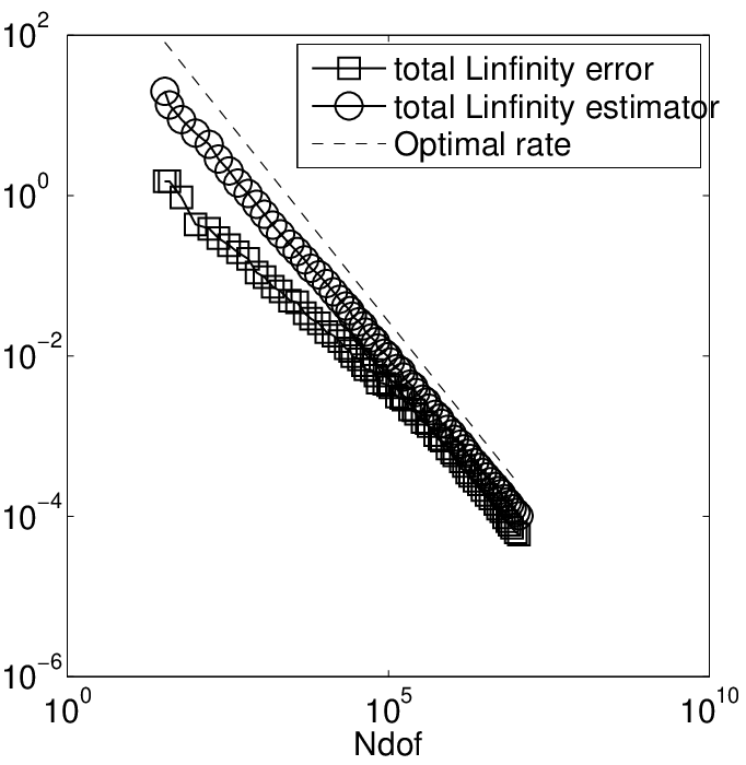
A sequence of adaptively refined meshes was generated from an initial mesh (consisting of 12 congruent triangles) by using a maximum strategy to mark elements for refinement. The number of degrees of freedom Ndof is three times the number of vertices in the mesh. Figure 1 shows the results and we can observe that, once the mesh has been sufficiently refined, the error and estimator converge at the optimal rate.

Refer to caption — Figure 1: The error $\|(e_{\bar{\mathsf{y}}},e_{\bar{\mathsf{p}}},e_{\bar{\mathsf{u}}})\|_{\Omega}$ and the estimator $\mathscr{E}(\bar{\mathsf{y}}_{\mathscr{T}},\bar{\mathsf{p}}_{\mathscr{T}},\bar{\mathsf{u}}_{\mathscr{T}};\mathscr{T})$ (left) and the 24th adaptively refined mesh (right).

Acknowledgements.

A. Allendes was supported in part by CONICYT through FONDECYT project 1170579. E. Otárola was supported in part by CONICYT through FONDECYT project 3160201. A. J. Salgado was supported in part by NSF grant DMS-1418784.

References

(1) Ainsworth, M., Oden, J.T.: A posteriori error estimation in finite element analysis. Wiley-Interscience, New York (2000)
(2) Allendes, A., Otárola, E., Rankin, R., Salgado, A.J.: An a posteriori error analysis for an optimal control problem with point sources. arXiv:1608.08137 (2017)
(3) Dari, E., Durán, R.G., Padra, C.: Maximum norm error estimators for three-dimensional elliptic problems. SIAM J. Numer. Anal. 37(2), 683–700 (2000)
(4) Demlow, A., Kopteva, N.: Maximum-norm a posteriori error estimates for singularly perturbed elliptic reaction-diffusion problems. Numer. Math. 133(4), 707–742 (2016)
(5) Ern, A., Guermond, J.L.: Theory and practice of finite elements. Springer, New York (2004)
(6) Jerison, D., Kenig, C.E.: The inhomogeneous Dirichlet problem in Lipschitz domains. J. Funct. Anal. 130(1), 161–219 (1995)
(7) Nochetto, R.H.: Pointwise a posteriori error estimates for elliptic problems on highly graded meshes. Math. Comp. 64(209), 1–22 (1995)
(8) Nochetto, R.H., Schmidt, A., Siebert, K.G., Veeser, A.: Pointwise a posteriori error estimates for monotone semi-linear equations. Numer. Math. 104(4), 515–538 (2006)
(9) Verfürth, R.: A posteriori error estimation techniques for finite element methods. Oxford University Press, Oxford (2013)

	$\displaystyle\\|\bar{\mathsf{u}}-\bar{\mathsf{u}}_{\mathscr{T}}\\|^{2}_{L^{2}(\Omega)}\lesssim$	$\displaystyle\\|\tilde{\mathsf{u}}-\bar{\mathsf{u}}_{\mathscr{T}}\\|_{L^{2}(\Omega)}^{2}+\\|\hat{\mathsf{y}}-\bar{\mathsf{y}}_{\mathscr{T}}\\|_{L^{2}(\Omega)}^{2}+\\|\hat{\mathsf{p}}-\bar{\mathsf{p}}_{\mathscr{T}}\\|_{L^{2}(\Omega)}^{2}$
	$\displaystyle\lesssim$	$\displaystyle\\|\tilde{\mathsf{u}}-\bar{\mathsf{u}}_{\mathscr{T}}\\|_{L^{\infty}(\Omega)}^{2}+\\|\hat{\mathsf{y}}-\bar{\mathsf{y}}_{\mathscr{T}}\\|_{L^{\infty}(\Omega)}^{2}+\\|\hat{\mathsf{p}}-\bar{\mathsf{p}}_{\mathscr{T}}\\|_{L^{\infty}(\Omega)}^{2}.$		(27)

	$\displaystyle\\|\bar{\mathsf{p}}-\bar{\mathsf{p}}_{\mathscr{T}}\\|_{L^{\infty}(\Omega)}^{2}\lesssim$	$\displaystyle\\|\bar{\mathsf{p}}-\hat{\mathsf{p}}\\|_{L^{\infty}(\Omega)}^{2}+\\|\hat{\mathsf{p}}-\bar{\mathsf{p}}_{\mathscr{T}}\\|_{L^{\infty}(\Omega)}^{2}$
	$\displaystyle\lesssim$	$\displaystyle\\|\hat{\mathsf{y}}-\bar{\mathsf{y}}_{\mathscr{T}}\\|_{L^{\infty}(\Omega)}^{2}+\\|\hat{\mathsf{p}}-\bar{\mathsf{p}}_{\mathscr{T}}\\|_{L^{\infty}(\Omega)}^{2}+\\|\tilde{\mathsf{u}}-\bar{\mathsf{u}}_{\mathscr{T}}\\|_{L^{\infty}(\Omega)}^{2}.$		(29)

		$\displaystyle\left\|\int_{T}\Delta\beta_{T}(\bar{\mathsf{y}}-\bar{\mathsf{y}}_{\mathscr{T}})\right\|$
	$\displaystyle\lesssim$	$\displaystyle\left(h_{T}^{d/2-1}\\|\nabla(\mathcal{P}_{\mathscr{T}}\mathsf{f}+\bar{\mathsf{u}}_{\mathscr{T}})\\|_{L^{2}(T)}+h_{T}^{d/2-2}\\|\mathcal{P}_{\mathscr{T}}\mathsf{f}+\bar{\mathsf{u}}_{\mathscr{T}}\\|_{L^{2}(T)}\right)\\|\bar{\mathsf{y}}-\bar{\mathsf{y}}_{\mathscr{T}}\\|_{L^{\infty}(T)}$
	$\displaystyle\lesssim$	$\displaystyle h_{T}^{d/2-2}\\|\mathcal{P}_{\mathscr{T}}\mathsf{f}+\bar{\mathsf{u}}_{\mathscr{T}}\\|_{L^{2}(T)}\\|\bar{\mathsf{y}}-\bar{\mathsf{y}}_{\mathscr{T}}\\|_{L^{\infty}(T)}.$

	$\displaystyle\left\|\int_{T}(\bar{\mathsf{u}}-\bar{\mathsf{u}}_{\mathscr{T}})\beta_{T}\right\|\lesssim$	$\displaystyle\\|\bar{\mathsf{u}}-\bar{\mathsf{u}}_{\mathscr{T}}\\|_{L^{2}(T)}\\|\mathcal{P}_{\mathscr{T}}\mathsf{f}+\bar{\mathsf{u}}_{\mathscr{T}}\\|_{L^{2}(T)}$
	$\displaystyle\lesssim$	$\displaystyle h_{T}^{d/2}\\|\bar{\mathsf{u}}-\bar{\mathsf{u}}_{\mathscr{T}}\\|_{L^{\infty}(T)}\\|\mathcal{P}_{\mathscr{T}}\mathsf{f}+\bar{\mathsf{u}}_{\mathscr{T}}\\|_{L^{2}(T)}$

		$\displaystyle\left\|\int_{S}\llbracket\nabla\bar{\mathsf{y}}_{\mathscr{T}}\cdot\nu\rrbracket\varphi_{S}\right\|$
	$\displaystyle\leq$	$\displaystyle\sum_{T^{\prime}\in\mathcal{N}_{S}}\int_{T^{\prime}}\|\mathsf{f}+\bar{\mathsf{u}}\|\varphi_{S}+\sum_{T^{\prime}\in\mathcal{N}_{S}}\int_{T^{\prime}}\|\bar{\mathsf{y}}-\bar{\mathsf{y}}_{\mathscr{T}}\|\|{\Delta}\varphi_{S}\|+\sum_{T^{\prime}\in\mathcal{N}_{S}}\sum_{S^{\prime}\in\mathscr{S}_{T^{\prime}}}\int_{S^{\prime}}\|\bar{\mathsf{y}}-\bar{\mathsf{y}}_{\mathscr{T}}\|\|\llbracket\nabla\varphi_{S}\cdot\nu\rrbracket\|$
	$\displaystyle\lesssim$	$\displaystyle\sum_{T^{\prime}\in\mathcal{N}_{S}}\|T^{\prime}\|^{1/2}\left(\\|\mathsf{f}+\bar{\mathsf{u}}_{\mathscr{T}}\\|_{L^{2}(T^{\prime})}+\|T^{\prime}\|^{1/2}\\|\bar{\mathsf{u}}-\bar{\mathsf{u}}_{\mathscr{T}}\\|_{L^{\infty}(T^{\prime})}\right)$
		$\displaystyle+\sum_{T^{\prime}\in\mathcal{N}_{S}}\left(h_{S}^{-2}\|T^{\prime}\|+h_{S}^{-1}\sum_{S^{\prime}\in\mathscr{S}_{T^{\prime}}}\|S^{\prime}\|\right)\\|\bar{\mathsf{y}}-\bar{\mathsf{y}}_{\mathscr{T}}\\|_{L^{\infty}(T^{\prime})}.$

Maximum–norm a posteriori error estimates for an optimal control problem

Abstract

Keywords:

MSC

1 Introduction

2 Notation

3 Optimal control problem

4 A posteriori error analysis: reliability

Theorem 4.1 (global reliability)

Proof

5 A posteriori error analysis: efficiency

Lemma 1 (local efficiency of ℰ𝗒\mathscr{E}_{\mathsf{y}})

Proof

Lemma 2 (local efficiency of ℰ𝗉\mathscr{E}_{\mathsf{p}})

Lemma 3 (local efficiency of ℰ𝗎\mathscr{E}_{\mathsf{u}})

Proof

Theorem 5.1 (local and global efficiency of ℰ\mathscr{E})

6 Numerical example

Acknowledgements.

References

Lemma 1 (local efficiency of $\mathscr{E}_{\mathsf{y}}$ )

Lemma 2 (local efficiency of $\mathscr{E}_{\mathsf{p}}$ )

Lemma 3 (local efficiency of $\mathscr{E}_{\mathsf{u}}$ )

Theorem 5.1 (local and global efficiency of $\mathscr{E}$ )