跳到论文正文
W Papers独立论文阅读器 arXiv:1711.06642 论文正文 计算阅读时间 · 0%
引用这篇论文根据当前论文元数据生成,正式投稿前建议核对。


License: arXiv.org perpetual non-exclusive license
arXiv:1711.06642v1 [stat.ME] 17 Nov 2017

Nonparametric independence testing via mutual information

Thomas B. Berrett    Richard J. Samworth Affiliation: Statistical Laboratory, University of Cambridge
Abstract

We propose a test of independence of two multivariate random vectors, given a sample from the underlying population. Our approach, which we call MINT, is based on the estimation of mutual information, whose decomposition into joint and marginal entropies facilitates the use of recently-developed efficient entropy estimators derived from nearest neighbour distances. The proposed critical values, which may be obtained from simulation (in the case where one marginal is known) or resampling, guarantee that the test has nominal size, and we provide local power analyses, uniformly over classes of densities whose mutual information satisfies a lower bound. Our ideas may be extended to provide a new goodness-of-fit tests of normal linear models based on assessing the independence of our vector of covariates and an appropriately-defined notion of an error vector. The theory is supported by numerical studies on both simulated and real data.

1 Introduction

Independence is a fundamental concept in statistics and many related fields, underpinning the way practitioners frequently think about model building, as well as much of statistical theory. Often we would like to assess whether or not the assumption of independence is reasonable, for instance as a method of exploratory data analysis (Steuer et al., 2002; Albert et al., 2015; Nguyen and Eisenstein, 2017), or as a way of evaluating the goodness-of-fit of a statistical model (Einmahl and van Keilegom, 2008). Testing independence and estimating dependence are well-established areas of statistics, with the related idea of the correlation between two random variables dating back to Francis Galton’s work at the end of the 19th century (Stigler, 1989), which was subsequently expanded upon by Karl Pearson (Pearson, 1920, e.g.). Since then many new measures of dependence have been developed and studied, each with its own advantages and disadvantages, and there is no universally accepted measure. For surveys of several measures, see, for example, Schweizer (1981), Joe (1989), Mari and Kotz (2001) and the references therein. We give an overview of more recently-introduced quantities below; see also Josse and Holmes (2016).

In addition to the applications mentioned above, dependence measures play an important role in independent component analysis (ICA), a special case of blind source separation, in which a linear transformation of the data is sought so that the transformed data is maximally independent; see e.g. Comon (1994), Bach and Jordan (2002), Miller and Fisher (2003) and Samworth and Yuan (2012). Here, independence tests may be carried out to check the convergence of an ICA algorithm and to validate the results (Wu, Yu and Li, 2009, e.g.). Further examples include feature selection, where one seeks a set of features which contains the maximum possible information about a response (Torkkola, 2003; Song et al., 2012), and the evaluation of the quality of a clustering in cluster analysis (Vinh, Epps and Bailey, 2010).

When dealing with discrete data, often presented in a contingency table, the independence testing problem is typically reduced to testing the equality of two discrete distributions via a chi-squared test. Here we will focus on the case of distributions that are absolutely continuous with respect to the relevant Lebesgue measure. Classical nonparametric approaches to measuring dependence and independence testing in such cases include Pearson’s correlation coefficient, Kendall’s tau and Spearman’s rank correlation coefficient. Though these approaches are widely used, they suffer from a lack of power against many alternatives; indeed Pearson’s correlation only measures linear relationships between variables, while Kendall’s tau and Spearman’s rank correlation coefficient measure monotonic relationships. Thus, for example, if XX has a symmetric distribution on the real line, and Y=X2Y=X^{2}, then the population quantities corresponding to these test statistics are zero in all three cases. Hoeffding’s test of independence (Hoeffding, 1948) is able to detect a wider class of departures from independence and is distribution-free under the null hypothesis but, as with these other classical methods, was only designed for univariate variables. Recent work of Weihs, Drton and Meinshausen (2017) has aimed to address some of computational challenges involved in extending these ideas to multivariate settings.

Recent research has focused on constructing tests that can be used for more complex data and that are consistent against wider classes of alternatives. The concept of distance covariance was introduced in Székely, Rizzo and Bakirov (2007) and can be expressed as a weighted L2L_{2} norm between the characteristic function of the joint distribution and the product of the marginal characteristic functions. This concept has also been studied in high dimensions (Székely and Rizzo, 2013; Yao, Zhang and Shao, 2017), and for testing independence of several random vectors (Fan et al., 2017). In Sejdinovic et al. (2013) tests based on distance covariance were shown to be equivalent to a reproducing kernel Hilbert space (RKHS) test for a specific choice of kernel. RKHS tests have been widely studied in the machine learning community, with early understanding of the subject given by Bach and Jordan (2002) and Gretton et al. (2005), in which the Hilbert–Schmidt independence criterion was proposed. These tests are based on embedding the joint distribution and product of the marginal distributions into a Hilbert space and considering the norm of their difference in this space. One drawback of the kernel paradigm here is the computational complexity, though Jitkrittum, Szabó and Gretton (2016) and Zhang et al. (2017) have recently attempted to address this issue. The performance of these methods may also be strongly affected by the choice of kernel. In another line of work, there is a large literature on testing independence based on an empirical copula process; see for example Kojadinovic and Holmes (2009) and the references therein. Other test statistics include those based on partitioning the sample space (Gretton and Györfi, 2010; Heller et al., 2016, e.g.). These have the advantage of being distribution-free under the null hypothesis, though their performance depends on the particular partition chosen.

We also remark that the basic independence testing problem has spawned many variants. For instance, Pfister et al. (2017) extend kernel tests to tests of mutual independence between a group of random vectors. Another important extension is to the problem of testing conditional independence, which is central to graphical modelling (Lauritzen, 1996) and also relevant to causal inference (Pearl, 2009). Existing tests of conditional independence include the proposals of Su and White (2008), Zhang et al. (2011) and Fan, Feng and Xia (2017).

To formalise the problem we consider, let XX and YY have (Lebesgue) densities fXf_{X} on ℝdX\mathbb{R}^{d_{X}} and fYf_{Y} on ℝdY\mathbb{R}^{d_{Y}} respectively, and let Z=(X,Y)Z=(X,Y) have density ff on ℝd\mathbb{R}^{d}, where d:=dX+dYd:=d_{X}+d_{Y}. Given independent and identically distributed copies Z1,…,ZnZ_{1},\ldots,Z_{n} of ZZ, we wish to test the null hypothesis that XX and YY are independent, denoted H0:X⟂⟂YH_{0}:X\perp\!\!\!\perp Y, against the alternative that XX and YY are not independent, written H1:X​⟂⟂YH_{1}:X\not\!\perp\!\!\!\perp Y. Our approach is based on constructing an estimator I^n=I^n​(Z1,…,Zn)\widehat{I}_{n}=\widehat{I}_{n}(Z_{1},\ldots,Z_{n}) of the mutual information I⁡(X,Y)I(X;Y) between XX and YY. Mutual information turns out to be a very attractive measure of dependence in this context; we review its definition and basic properties in Section 2 below. In particular, its decomposition into joint and marginal entropies (see (1) below) facilitates the use of recently-developed efficient entropy estimators derived from nearest neighbour distances (Berrett, Samworth and Yuan, 2017).

The next main challenge is to identify an appropriate critical value for the test. In the simpler setting where either of the marginals fXf_{X} and fYf_{Y} is known, a simulation-based approach can be employed to yield a test of any given size q∈(0,1)q\in(0,1). We further provide regularity conditions under which the power of our test converges to 11 as n→∞n\rightarrow\infty, uniformly over classes of alternatives with I⁡(X,Y)≥bnI(X;Y)\geq b_{n}, say, where we may even take bn=o(n−1/2)b_{n}=o(n^{-1/2}). To the best of our knowledge this is the first time that such a local power analysis has been carried out for an independence test for multivariate data. When neither marginal is known, we obtain our critical value via a permutation approach, again yielding a test of the nominal size. Here, under our regularity conditions, the test is uniformly consistent (has power converging to 1) against alternatives whose mutual information is bounded away from zero. We call our test MINT, short for Mutual Information Test; it is implemented in the R package IndepTest (Berrett, Grose and Samworth, 2017).

As an application of these ideas, we are able to introduce new goodness-of-fit tests of normal linear models based on assessing the independence of our vector of covariates and an appropriately-defined notion of an error vector. Such tests do not follow immediately from our earlier work, because we do not observe realisations of the error vector directly; instead, we only have access to residuals from a fitted model. Nevertheless, we are able to provide rigorous justification, again in the form of a local analysis, for our approach. It seems that, when fitting normal linear models, current standard practice in the applied statistics community for assessing goodness-of-fit is based on visual inspection of diagnostic plots such as those provided by the plot command in R when applied to an object of class lm. Our aim, then, is to augment the standard toolkit by providing a formal basis for inference regarding the validity of the model. Related work here includes Neumeyer (2009), Neumeyer and Van Keilegom (2010), Müller, Schick and Wefelmeyer (2012), Sen and Sen (2014) and Shah and Bühlmann (2017).

The remainder of the paper is organised as follows: after reviewing the concept of mutual information in Section 2.1, we explain in Section 2.2 how it can be estimated effectively from data using efficient entropy estimators. Our new tests, for the cases where one of the marginals is known and where they are both unknown, are introduced in Sections 3 and 4 respectively. The regression setting is considered in Section 5, and numerical studies on both simulated and real data are presented in Section 6. Proofs are given in Section 7.

The following notation is used throughout. For a generic dimension D∈ℕD\in\mathbb{N}, let λD\lambda_{D} and ∥⋅∥\|\cdot\| denote Lebesgue measure and the Euclidean norm on ℝD\mathbb{R}^{D} respectively. If f=d​μ/d​λDf=d\mu/d\lambda_{D} and g=d​ν/d​λDg=d\nu/d\lambda_{D} are densities on ℝD\mathbb{R}^{D} with respect to λD\lambda_{D}, we write f≪gf\ll g if μ≪ν\mu\ll\nu. For z∈ℝDz\in\mathbb{R}^{D} and r∈[0,∞)r\in[0,\infty), we write Bz​(r):={w∈ℝD:‖w−z‖≤r}B_{z}(r):=\{w\in\mathbb{R}^{D}:\|w-z\|\leq r\} and Bz∘​(r):=Bz​(r)∖{z}B_{z}^{\circ}(r):=B_{z}(r)\setminus\{z\}. We write λmin​(A)\lambda_{\min}(A) for the smallest eigenvalue of a positive definite matrix AA, and ‖B‖F\|B\|_{\mathrm{F}} for the Frobenius norm of a matrix BB.

2 Mutual information

2.1 Definition and basic properties

Retaining our notation from the introduction, let 𝒵:={(x,y):f⁡(x,y)>0}\mathcal{Z}:=\{(x,y):f(x,y)>0\}. A very natural measure of dependence is the mutual information between XX and YY, defined to be

I⁡(X,Y)=I⁡(f):=∫𝒵f⁡(x,y)​log⁡f⁡(x,y)fX​(x)​fY​(y)​d​λd​(x,y),I(X;Y)=I(f):=\int_{\mathcal{Z}}f(x,y)\log\frac{f(x,y)}{f_{X}(x)f_{Y}(y)}\,d\lambda_{d}(x,y),

when f≪fX​fYf\ll f_{X}f_{Y}, and defined to be ∞\infty otherwise. This is the Kullback–Leibler divergence between the joint distribution of (X,Y)(X,Y) and the product of the marginal distributions, so is non-negative, and equal to zero if and only if XX and YY are independent. Another attractive feature of mutual information as a measure of dependence is that it is invariant to smooth, invertible transformations of XX and YY. Indeed, suppose that 𝒳:={x:fX​(x)>0}\mathcal{X}:=\{x:f_{X}(x)>0\} is an open subset of ℝdX\mathbb{R}^{d_{X}} and ϕ:𝒳→𝒳′\phi:\mathcal{X}\rightarrow\mathcal{X}^{\prime} is a continuously differentiable bijection whose inverse ϕ−1\phi^{-1} has Jacobian determinant J⁡(x′)J(x^{\prime}) that never vanishes on 𝒳′\mathcal{X}^{\prime}. Let Φ:𝒳×𝒴→𝒳′×𝒴\Phi:\mathcal{X}\times\mathcal{Y}\rightarrow\mathcal{X}^{\prime}\times\mathcal{Y} be given by Φ⁡(x,y):=(ϕ⁡(x),y)\Phi(x,y):=\bigl(\phi(x),y\bigr), so that Φ−1​(x′,y)=(ϕ−1​(x′),y)\Phi^{-1}(x^{\prime},y)=\bigl(\phi^{-1}(x^{\prime}),y) also has Jacobian determinant J⁡(x′)J(x^{\prime}). Then Φ⁡(X,Y)\Phi(X,Y) has density g⁡(x′,y)=f⁡(ϕ−1​(x′),y)​|J⁡(x′)|g(x^{\prime},y)=f\bigl(\phi^{-1}(x^{\prime}),y\bigr)|J(x^{\prime})| on Φ⁡(𝒵)\Phi(\mathcal{Z}) and X′=ϕ⁡(X)X^{\prime}=\phi(X) has density gX′​(x′)=fX​(ϕ−1​(x′))​|J⁡(x′)|g_{X^{\prime}}(x^{\prime})=f_{X}\bigl(\phi^{-1}(x^{\prime})\bigr)|J(x^{\prime})| on 𝒳′\mathcal{X}^{\prime}. It follows that

I⁡(ϕ⁡(X),Y)\displaystyle I\bigl(\phi(X);Y\bigr) =∫Φ⁡(𝒵)g⁡(x′,y)​log⁡g⁡(x′,y)gX′​(x′)​fY​(y)​d​λd​(x′,y)\displaystyle=\int_{\Phi(\mathcal{Z})}g(x^{\prime},y)\log\frac{g(x^{\prime},y)}{g_{X^{\prime}}(x^{\prime})f_{Y}(y)}\,d\lambda_{d}(x^{\prime},y)
=∫Φ⁡(𝒵)g⁡(x′,y)​log⁡f⁡(ϕ−1​(x′),y)fX​(ϕ−1​(x′))​fY​(y)​d​λd​(x′,y)=I⁡(X,Y).\displaystyle=\int_{\Phi(\mathcal{Z})}g(x^{\prime},y)\log\frac{f\bigl(\phi^{-1}(x^{\prime}),y\bigr)}{f_{X}\bigl(\phi^{-1}(x^{\prime})\bigr)f_{Y}(y)}\,d\lambda_{d}(x^{\prime},y)=I(X;Y).

This means that mutual information is nonparametric in the sense of Weihs, Drton and Meinshausen (2017), whereas several other measures of dependence, including distance covariance, RKHS measures and correlation-based notions are not in general. Under a mild assumption, the mutual information between XX and YY can be expressed in terms of their joint and marginal entropies; more precisely, writing 𝒴:={y:fY​(y)>0}\mathcal{Y}:=\{y:f_{Y}(y)>0\}, and provided that each of H⁡(X,Y)H(X,Y), H⁡(X)H(X) and H⁡(Y)H(Y) are finite,

I⁡(X,Y)\displaystyle I(X;Y) =∫𝒵f​log⁡f​d​λd−∫𝒳fX​log​fX​d​μdX−∫𝒴fY​log​fY​d​μdY\displaystyle=\int_{\mathcal{Z}}f\log f\,d\lambda_{d}-\int_{\mathcal{X}}f_{X}\log f_{X}\,d\mu_{d_{X}}-\int_{\mathcal{Y}}f_{Y}\log f_{Y}\,d\mu_{d_{Y}}
=:−H⁡(X,Y)+H⁡(X)+H⁡(Y).\displaystyle=:-H(X,Y)+H(X)+H(Y). (1)

Thus, mutual information estimators can be constructed from entropy estimators.

Moreover, the concept of mutual information is easily generalised to more complex situations. For instance, suppose now that (X,Y,W)(X,Y,W) has joint density ff on ℝd+dW\mathbb{R}^{d+d_{W}}, and let f(X,Y)|W(⋅|w)f_{(X,Y)|W}(\cdot|w), fX|W(⋅|w)f_{X|W}(\cdot|w) and fY|W(⋅|w)f_{Y|W}(\cdot|w) denote the joint conditional density of (X,Y)(X,Y) given W=wW=w and the conditional densities of XX given W=wW=w and YY given W=wW=w respectively. When f(X,Y)|W(⋅,⋅|w)≪fX|W(⋅|w)fY|W(⋅|w)f_{(X,Y)|W}(\cdot,\cdot|w)\ll f_{X|W}(\cdot|w)f_{Y|W}(\cdot|w) for each ww in the support of WW, the conditional mutual information between XX and YY given WW is defined as

I⁡(X;Y|W):=∫𝒲f⁡(x,y,w)​log⁡f(X,Y)|W​(x,y|w)fX|W​(x|w)​fY|W​(y|w)​d​λd+dW​(x,y,w),I(X;Y|W):=\int_{\mathcal{W}}f(x,y,w)\log\frac{f_{(X,Y)|W}(x,y|w)}{f_{X|W}(x|w)f_{Y|W}(y|w)}\,d\lambda_{d+d_{W}}(x,y,w),

where 𝒲:={(x,y,w):f⁡(x,y,w)>0}\mathcal{W}:=\{(x,y,w):f(x,y,w)>0\}. This can similarly be written as

I⁡(X;Y|W)=H⁡(X,W)+H⁡(Y,W)−H⁡(X,Y,W)−H⁡(W),I(X;Y|W)=H(X,W)+H(Y,W)-H(X,Y,W)-H(W),

provided each of the summands is finite.

Finally, we mention that the concept of mutual information easily generalises to situations with pp random vectors. In particular, suppose that X1,…,XpX_{1},\ldots,X_{p} have joint density ff on ℝd\mathbb{R}^{d}, where d=d1+…+dpd=d_{1}+\ldots+d_{p} and that XjX_{j} has marginal density fjf_{j} on ℝdj\mathbb{R}^{d_{j}}. Then, when f≪f1​…​fpf\ll f_{1}\ldots f_{p}, and writing 𝒳p:={(x1,…,xp)∈ℝd:f⁡(x1,…,xp)>0}\mathcal{X}_{p}:=\{(x_{1},\ldots,x_{p})\in\mathbb{R}^{d}:f(x_{1},\ldots,x_{p})>0\}, we can define

I⁡(X1,…,Xp)\displaystyle I(X_{1};\ldots;X_{p}) :=∫𝒳pf⁡(x1,…,xp)​log⁡f⁡(x1,…,xp)f1​(x1)​…​fp​(xp)​d​λd​(x1,…,xp)\displaystyle:=\int_{\mathcal{X}_{p}}f(x_{1},\ldots,x_{p})\log\frac{f(x_{1},\ldots,x_{p})}{f_{1}(x_{1})\ldots f_{p}(x_{p})}\,d\lambda_{d}(x_{1},\ldots,x_{p})
=∑j=1pH⁡(Xj)−H⁡(X1,…,Xp),\displaystyle=\sum_{j=1}^{p}H(X_{j})-H(X_{1},\ldots,X_{p}),

with the second equality holding provided that each of the entropies is finite. The tests we introduce in Sections 3 and 4 therefore extend in a straightforward manner to tests of independence of several random vectors.

2.2 Estimation of mutual information

For i=1,…,ni=1,\dots,n, let Z(1),i,…,Z(n−1),iZ_{(1),i},\ldots,Z_{(n-1),i} denote a permutation of {Z1,…,Zn}∖{Zi}\{Z_{1},\ldots,Z_{n}\}\setminus\{Z_{i}\} such that ‖Z(1),i−Zi‖≤…≤‖Z(n−1),i−Zi‖\|Z_{(1),i}-Z_{i}\|\leq\ldots\leq\|Z_{(n-1),i}-Z_{i}\|. For conciseness, we let

ρ(k),i:=‖Z(k),i−Zi‖\rho_{(k),i}:=\|Z_{(k),i}-Z_{i}\|

denote the distance between ZiZ_{i} and the kkth nearest neighbour of ZiZ_{i}. To estimate the unknown entropies, we will use a weighted version of the Kozachenko–Leonenko estimator (Kozachenko and Leonenko, 1987). For k=kZ∈{1,…,n−1}k=k^{Z}\in\{1,\ldots,n-1\} and weights w1Z,…,wkZw_{1}^{Z},\ldots,w_{k}^{Z} satisfying ∑j=1kwjZ=1\sum_{j=1}^{k}w_{j}^{Z}=1, this is defined as

H^nZ=H^n,kd,wZ​(Z1,…,Zn):=1n​∑i=1n∑j=1kwjZ​log⁡(ρ(j),id​Vd​(n−1)eΨ⁡(j)),\widehat{H}_{n}^{Z}=\widehat{H}_{n,k}^{d,w^{Z}}(Z_{1},\ldots,Z_{n}):=\frac{1}{n}\sum_{i=1}^{n}\sum_{j=1}^{k}w_{j}^{Z}\log\biggl(\frac{\rho_{(j),i}^{d}V_{d}(n-1)}{e^{\Psi(j)}}\biggr),

where Vd:=πd/2/Γ⁡(1+d/2)V_{d}:=\pi^{d/2}/\Gamma(1+d/2) denotes the volume of the unit dd-dimensional Euclidean ball and where Ψ\Psi denotes the digamma function. Berrett, Samworth and Yuan (2017) provided conditions on kk, w1Z,…,wkZw_{1}^{Z},\ldots,w_{k}^{Z} and the underlying data generating mechanism under which H^nZ\widehat{H}_{n}^{Z} is an efficient estimator of H⁡(Z)H(Z) (in the sense that its asymptotic normalised squared error risk achieves the local asymptotic minimax lower bound) in arbitrary dimensions. With estimators H^nX\widehat{H}_{n}^{X} and H^nY\widehat{H}_{n}^{Y} of H⁡(X)H(X) and H⁡(Y)H(Y) defined analogously as functions of (X1,…,Xn)(X_{1},\ldots,X_{n}) and (Y1,…,Yn)(Y_{1},\ldots,Y_{n}) respectively, we can use (1) to define an estimator of mutual information by

I^n=I^n​(Z1,…,Zn)=H^nX+H^nY−H^nZ.\widehat{I}_{n}=\widehat{I}_{n}(Z_{1},\ldots,Z_{n})=\widehat{H}_{n}^{X}+\widehat{H}_{n}^{Y}-\widehat{H}_{n}^{Z}. (2)

Having identified an appropriate mutual information estimator, we turn our attention in the next two sections to obtaining appropriate critical values for our independence tests.

3 The case of one known marginal distribution

In this section, we consider the case where at least one of fXf_{X} and fYf_{Y} in known (in our experience, little is gained by knowledge of the second marginal density), and without loss of generality, we take the known marginal to be fYf_{Y}. We further assume that we can generate independent and identically distributed copies of YY, denoted {Yi(b):i=1,…,n,b=1,…,B}\{Y_{i}^{(b)}:i=1,\ldots,n,b=1,\ldots,B\}, independently of Z1,…,ZnZ_{1},\ldots,Z_{n}. Our test in this setting, which we refer to as MINTknown (or MINTknown(q)(q) when the nominal size q∈(0,1)q\in(0,1) needs to be made explicit), will reject H0H_{0} for large values of I^n\widehat{I}_{n}. The ideal critical value, if both marginal densities were known, would therefore be

Cq(n):=inf{r∈ℝ:ℙfX​fY​(I^n>r)≤q}.C_{q}^{(n)}:=\inf\{r\in\mathbb{R}:\mathbb{P}_{f_{X}f_{Y}}(\widehat{I}_{n}>r)\leq q\}.

Using our pseudo-data {Yi(b):i=1,…,n,b=1,…,B}\{Y_{i}^{(b)}:i=1,\ldots,n,b=1,\ldots,B\}, generated as described above, we define the statistics

I^n(b)=I^n​((X1,Y1(b)),…,(Xn,Yn(b)))\widehat{I}_{n}^{(b)}=\widehat{I}_{n}\bigl((X_{1},Y_{1}^{(b)}),\ldots,(X_{n},Y_{n}^{(b)})\bigr)

for b=1,…,Bb=1,\ldots,B. Motivated by the fact that these statistics have the same distribution as I^n\widehat{I}_{n} under H0H_{0}, we can estimate the critical value Cq(n)C_{q}^{(n)} by

C^q(n),B:=inf{r∈ℝ:1B+1∑b=0B𝟙{I^n(b)≥r}≤q},\widehat{C}_{q}^{(n),B}:=\inf\biggl\{r\in\mathbb{R}:\frac{1}{B+1}\sum_{b=0}^{B}\mathbbm{1}_{\{\widehat{I}_{n}^{(b)}\geq r\}}\leq q\biggr\},

the (1−q)(1-q)th quantile of {I^n(0),…,I^n(B)}\{\widehat{I}_{n}^{(0)},\ldots,\widehat{I}_{n}^{(B)}\}, where I^n(0):=I^n\widehat{I}_{n}^{(0)}:=\widehat{I}_{n}. The following lemma justifies this critical value estimate.

Lemma 1.

For any q∈(0,1)q\in(0,1) and B∈ℕB\in\mathbb{N}, the MINTknown(q)(q) test that rejects H0H_{0} if and only if I^n>C^q(n),B\widehat{I}_{n}>\widehat{C}_{q}^{(n),B} has size at most qq, in the sense that

supk∈{1,…,n−1}sup(X,Y):I⁡(X,Y)=0ℙ(I^n>C^q(n),B)≤q,\sup_{k\in\{1,\ldots,n-1\}}\sup_{(X,Y):I(X;Y)=0}\mathbb{P}\bigl(\widehat{I}_{n}>\widehat{C}_{q}^{(n),B}\bigr)\leq q,

where the inner supremum is over all joint distributions of pairs (X,Y)(X,Y) with I⁡(X,Y)=0I(X;Y)=0.

An interesting feature of MINTknown, which is apparent from the proof of Lemma 1, is that there is no need to calculate H^nX\widehat{H}_{n}^{X} in (1), either on the original data, or on the pseudo-data sets {(X1,Y1(b)),…,(Xn,Yn(b)):b=1,…,B}\{(X_{1},Y_{1}^{(b)}),\ldots,(X_{n},Y_{n}^{(b)}):b=1,\ldots,B\}. This is because in the decomposition of the event {I^n(b)≥I^n}\{\widehat{I}_{n}^{(b)}\geq\widehat{I}_{n}\} into entropy estimates, H^nX\widehat{H}_{n}^{X} appears on both sides of the inequality, so it cancels. This observation somewhat simplifies our assumptions and analysis, as well as reducing the number of tuning parameters that need to be chosen.

The remainder of this section is devoted to a rigorous study of the power of MINTknown that is compatible with a sequence of local alternatives (fn)(f_{n}) having mutual information In→0I_{n}\rightarrow 0. To this end, we first define the classes of alternatives that we consider; these parallel the classes introduced by Berrett, Samworth and Yuan (2017) in the context of entropy estimation. Let ℱd\mathcal{F}_{d} denote the class of all density functions with respect to Lebesgue measure on ℝd\mathbb{R}^{d}. For f∈ℱdf\in\mathcal{F}_{d} and α>0\alpha>0, let

μα​(f):=∫ℝd‖z‖α​f​(z)​𝑑z.\mu_{\alpha}(f):=\int_{\mathbb{R}^{d}}\|z\|^{\alpha}f(z)\,dz.

Now let 𝒜\mathcal{A} denote the class of decreasing functions a:(0,∞)→[1,∞)a:(0,\infty)\rightarrow[1,\infty) satisfying a⁡(δ)=o⁡(δ−ϵ)a(\delta)=o(\delta^{-\epsilon}) as δ↘0\delta\searrow 0, for every ϵ>0\epsilon>0. If a∈𝒜a\in\mathcal{A}, β>0\beta>0, f∈ℱdf\in\mathcal{F}_{d} is m:=(⌈β⌉−1CLOSEm:=(\lceil\beta\rceil-1)-times differentiable and z∈𝒵z\in\mathcal{Z}, we define ra(z):={8d1/2a(f(z))}−1/(β∧1)r_{a}(z):=\{8d^{1/2}a(f(z))\}^{-1/(\beta\wedge 1)} and

Mf,a,β​(z):=max⁡{maxt=1,…,m⁡‖f(t)​(z)‖f⁡(z),supw∈Bz∘​(ra​(z))‖f(m)​(w)−f(m)​(z)‖f⁡(z)​‖w−z‖β−m}.M_{f,a,\beta}(z):=\max\biggl\{\max_{t=1,\ldots,m}\frac{\|f^{(t)}(z)\|}{f(z)}\,,\,\sup_{w\in B_{z}^{\circ}(r_{a}(z))}\frac{\|f^{(m)}(w)-f^{(m)}(z)\|}{f(z)\|w-z\|^{\beta-m}}\biggr\}.

The quantity Mf,a,β​(z)M_{f,a,\beta}(z) measures the smoothness of derivatives of ff in neighbourhoods of zz, relative to f⁡(z)f(z) itself. Note that these neighbourhoods of zz are allowed to become smaller when f⁡(z)f(z) is small. Finally, for Θ:=(0,∞)4×𝒜\Theta:=(0,\infty)^{4}\times\mathcal{A}, and θ=(α,β,ν,γ,a)∈Θ\theta=(\alpha,\beta,\nu,\gamma,a)\in\Theta, let

ℱd,θ:={f∈ℱd:μα(f)≤ν,∥f∥∞≤γ,supz:f⁡(z)≥δMf,a,β(z)≤a(δ)∀δ>0}.\mathcal{F}_{d,\theta}:=\biggl\{f\in\mathcal{F}_{d}:\mu_{\alpha}(f)\leq\nu,\|f\|_{\infty}\leq\gamma,\sup_{z:f(z)\geq\delta}M_{f,a,\beta}(z)\leq a(\delta)\ \forall\delta>0\biggr\}.

Berrett, Samworth and Yuan (2017) show that all Gaussian and multivariate-tt densities (amongst others) belong to ℱd,θ\mathcal{F}_{d,\theta} for appropriate θ∈Θ\theta\in\Theta.

Now, for dX,dY∈ℕd_{X},d_{Y}\in\mathbb{N} and ϑ=(θ,θY)∈Θ2\vartheta=(\theta,\theta_{Y})\in\Theta^{2}, define

ℱdX,dY,ϑ:={f∈ℱdX+dY,θ:fY∈ℱdY,θY,fXfY∈ℱdX+dY,θ}\mathcal{F}_{d_{X},d_{Y},\vartheta}:=\Bigl\{f\in\mathcal{F}_{d_{X}+d_{Y},\theta}:f_{Y}\in\mathcal{F}_{d_{Y},\theta_{Y}},f_{X}f_{Y}\in\mathcal{F}_{d_{X}+d_{Y},\theta}\Bigr\}

and, for b≥0b\geq 0, let

ℱdX,dY,ϑ​(b):={f∈ℱdX,dY,ϑ:I⁡(f)>b}.\mathcal{F}_{d_{X},d_{Y},\vartheta}(b):=\Bigl\{f\in\mathcal{F}_{d_{X},d_{Y},\vartheta}:I(f)>b\Bigr\}.

Thus, ℱdX,dY,ϑ​(b)\mathcal{F}_{d_{X},d_{Y},\vartheta}(b) consists of joint densities whose mutual information is greater than bb. In Theorem 2 below, we will show that for a suitable choice of b=bnb=b_{n} and for certain ϑ∈Θ2\vartheta\in\Theta^{2}, the power of the test defined in Lemma 1 converges to 1, uniformly over ℱdX,dY,ϑ​(b)\mathcal{F}_{d_{X},d_{Y},\vartheta}(b).

Before we can state this result, however, we must define the allowable choices of kk and the weight vectors. Given d∈ℕd\in\mathbb{N} and θ=(α,β,γ,ν,a)∈Θ\theta=(\alpha,\beta,\gamma,\nu,a)\in\Theta let

τ1​(d,θ):=min⁡{2​α5​α+3​d,α−d2​α,4​(β∧1)4​(β∧1)+3​d}\tau_{1}(d,\theta):=\min\biggl\{\frac{2\alpha}{5\alpha+3d}\,,\,\frac{\alpha-d}{2\alpha}\,,\,\frac{4(\beta\wedge 1)}{4(\beta\wedge 1)+3d}\biggr\}

and

τ2​(d,θ):=min⁡{1−d2​β, 1−d/4⌊d/4⌋+1}\tau_{2}(d,\theta):=\min\biggl\{1-\frac{d}{2\beta}\,,\,1-\frac{d/4}{\lfloor d/4\rfloor+1}\biggr\}

Note that mini=1,2⁡τi​(d,θ)>0\min_{i=1,2}\tau_{i}(d,\theta)>0 if and only if both α>d\alpha>d and β>d/2\beta>d/2. Finally, for k∈ℕk\in\mathbb{N}, let

𝒲(k):={w=(w1,…,wk)T∈ℝk:\displaystyle\mathcal{W}^{(k)}:=\biggl\{w=(w_{1},\ldots,w_{k})^{T}\in\mathbb{R}^{k}: ∑j=1kwj​Γ⁡(j+2​ℓ/d)Γ⁡(j)=0for​ℓ=1,…,⌊d/4⌋\displaystyle\sum_{j=1}^{k}w_{j}\frac{\Gamma(j+2\ell/d)}{\Gamma(j)}=0\quad\text{for}\,\,\ell=1,\ldots,\lfloor d/4\rfloor
∑j=1kwj=1andwj=0ifj∉{⌊k/d⌋,⌊2k/d⌋,…,k}}.\displaystyle\sum_{j=1}^{k}w_{j}=1\,\text{and}\,\,w_{j}=0\,\,\text{if}\,j\notin\{\lfloor k/d\rfloor,\lfloor 2k/d\rfloor,\ldots,k\}\biggr\}.

Thus, our weights sum to 1; the other constraints ensure that the dominant contributions to the bias of the unweighted Kozachenko–Leonenko estimator cancel out to sufficiently high order, and that the corresponding jjth nearest neighbour distances are not too highly correlated.

Theorem 2.

Fix dX,dY∈ℕd_{X},d_{Y}\in\mathbb{N}, set d=dX+dYd=d_{X}+d_{Y} and fix ϑ=(θ,θY)∈Θ2\vartheta=(\theta,\theta_{Y})\in\Theta^{2} with

min⁡{τ1​(d,θ),τ1​(dY,θY),τ2​(d,θ),τ2​(dY,θY)}>0.\min\Bigl\{\tau_{1}(d,\theta)\,,\,\tau_{1}(d_{Y},\theta_{Y})\,,\,\tau_{2}(d,\theta)\,,\,\tau_{2}(d_{Y},\theta_{Y})\Bigr\}>0.

Let k0∗=k0,n∗,kY∗=kY,n∗k_{0}^{*}=k_{0,n}^{*},k_{Y}^{*}=k_{Y,n}^{*} and k∗=kn∗k^{*}=k_{n}^{*} denote any deterministic sequences of positive integers with k0∗≤min⁡{kY∗,k∗}k_{0}^{*}\leq\min\{k_{Y}^{*},k^{*}\}, with k0∗/log5⁡n→∞k_{0}^{*}/\log^{5}n\rightarrow\infty and with

max⁡{k∗nτ1​(d,θ)−ϵ,kY∗nτ1​(dY,θY)−ϵ,k∗nτ2​(d,θ),kY∗nτ2​(dY,θY)}→0\max\biggl\{\frac{k^{*}}{n^{\tau_{1}(d,\theta)-\epsilon}}\,,\,\frac{k_{Y}^{*}}{n^{\tau_{1}(d_{Y},\theta_{Y})-\epsilon}}\,,\,\frac{k^{*}}{n^{\tau_{2}(d,\theta)}}\,,\,\frac{k_{Y}^{*}}{n^{\tau_{2}(d_{Y},\theta_{Y})}}\biggr\}\rightarrow 0

for some ϵ>0\epsilon>0. Also suppose that wY=wY(kY)∈𝒲(kY)w_{Y}=w_{Y}^{(k_{Y})}\in\mathcal{W}^{(k_{Y})} and w=w(k)∈𝒲(k)w=w^{(k)}\in\mathcal{W}^{(k)}, and that lim supnmax⁡(‖w‖,‖wY‖)<∞\limsup_{n}\max(\|w\|,\|w_{Y}\|)<\infty. Then there exists a sequence (bn)(b_{n}) such that bn=o(n−1/2)b_{n}=o(n^{-1/2}) and with the property that for each q∈(0,1)q\in(0,1) and any sequence (Bn∗)(B_{n}^{*}) with Bn∗→∞B_{n}^{*}\rightarrow\infty,

infBn≥Bn∗infkY∈{k0∗,…,kY∗}k∈{k0∗,…,k∗}inff∈ℱdX,dY,ϑ​(bn)ℙf​(I^n>C^q(n),Bn)→1.\inf_{B_{n}\geq B_{n}^{*}}\inf_{\begin{subarray}{c}k_{Y}\in\{k_{0}^{*},\ldots,k_{Y}^{*}\}\\ k\in\{k_{0}^{*},\ldots,k^{*}\}\end{subarray}}\inf_{f\in\mathcal{F}_{d_{X},d_{Y},\vartheta}(b_{n})}\mathbb{P}_{f}(\widehat{I}_{n}>\widehat{C}_{q}^{(n),B_{n}})\rightarrow 1.

Theorem 2 provides a strong guarantee on the ability of MINTknown to detect alternatives, uniformly over classes whose mutual information is at least bnb_{n}, where we may even have bn=o(n−1/2)b_{n}=o(n^{-1/2}).

4 The case of unknown marginal distributions

We now consider the setting in which the marginal distributions of both XX and YY are unknown. Our test statistic remains the same, but now we estimate the critical value by permuting our sample in an attempt to mimic the behaviour of the test statistic under H0H_{0}. More explicity, for some B∈ℕB\in\mathbb{N}, we propose independently of (X1,Y1),…,(Xn,Yn)(X_{1},Y_{1}),\ldots,(X_{n},Y_{n}) to simulate independent random variables τ1,…,τB\tau_{1},\ldots,\tau_{B} uniformly from SnS_{n}, the permutation group of {1,…,n}\{1,\ldots,n\}, and for b=1,…,Bb=1,\ldots,B, set Zi(b):=(Xi,Yτb​(i))Z_{i}^{(b)}:=(X_{i},Y_{\tau_{b}(i)}) and I~n(b):=I^n​(Z1(b),…,Zn(b))\tilde{I}_{n}^{(b)}:=\widehat{I}_{n}(Z_{1}^{(b)},\ldots,Z_{n}^{(b)}). For q∈(0,1)q\in(0,1), we can now estimate Cq(n)C_{q}^{(n)} by

C~q(n),B:=inf{r∈ℝ:1B+1∑b=0B𝟙{I~n(b)≥r}≤q},\tilde{C}_{q}^{(n),B}:=\inf\biggl\{r\in\mathbb{R}:\frac{1}{B+1}\sum_{b=0}^{B}\mathbbm{1}_{\{\tilde{I}_{n}^{(b)}\geq r\}}\leq q\biggr\},

where I~n(0):=I^n\tilde{I}_{n}^{(0)}:=\widehat{I}_{n}, and refer to the test that rejects H0H_{0} if and only if I^n>C~q(n),B\widehat{I}_{n}>\tilde{C}_{q}^{(n),B} as MINTunknown(q)(q).

Lemma 3.

For any q∈(0,1)q\in(0,1) and B∈ℕB\in\mathbb{N}, the MINTunknown(q)(q) test has size at most qq:

supk∈{1,…,n−1}sup(X,Y):I⁡(X,Y)=0ℙ(I^n>C~q(n),B)≤q.\sup_{k\in\{1,\ldots,n-1\}}\sup_{(X,Y):I(X;Y)=0}\mathbb{P}\bigl(\widehat{I}_{n}>\tilde{C}_{q}^{(n),B}\bigr)\leq q.

Note that I^n>C~q(n),B\widehat{I}_{n}>\tilde{C}_{q}^{(n),B} if and only if

1B+1∑b=0B𝟙{I~n(b)≥I^n}≤q.\frac{1}{B+1}\sum_{b=0}^{B}\mathbbm{1}_{\{\tilde{I}_{n}^{(b)}\geq\widehat{I}_{n}\}}\leq q. (3)

This shows that estimating either of the marginal entropies is unnecessary to carry out the test, since I~n(b)−I^n=H^nZ−H~n(b)\tilde{I}_{n}^{(b)}-\widehat{I}_{n}=\widehat{H}_{n}^{Z}-\tilde{H}_{n}^{(b)}, where H~n(b):=H^n,kd,wZ​(Z1(b),…,Zn(b))\tilde{H}_{n}^{(b)}:=\widehat{H}_{n,k}^{d,w^{Z}}(Z_{1}^{(b)},\ldots,Z_{n}^{(b)}) is the weighted Kozachenko–Leonenko joint entropy estimator based on the permuted data.

We now study the power of MINTunknown, and begin by introducing the classes of marginal densities that we consider. To define an appropriate notion of smoothness, for z∈{w:g⁡(w)>0}=:𝒲z\in\{w:g(w)>0\}=:\mathcal{W}, g∈ℱdg\in\mathcal{F}_{d} and δ>0\delta>0, let

rz,g,δ:={δ​eΨ⁡(k)Vd​(n−1)​g​(z)}1/d.r_{z,g,\delta}:=\biggl\{\frac{\delta e^{\Psi(k)}}{V_{d}(n-1)g(z)}\biggr\}^{1/d}. (4)

Now, for AA belonging to the class of Borel subsets of 𝒲\mathcal{W}, denoted ℬ⁡(𝒲)\mathcal{B}(\mathcal{W}), define

Mg​(A):=supδ∈(0,2]supz∈A|1Vd​rz,g,δd​g​(z)​∫Bz​(rz,g,δ)g​d​λd−1|.M_{g}(A):=\sup_{\delta\in(0,2]}\sup_{z\in A}\biggl|\frac{1}{V_{d}r_{z,g,\delta}^{d}g(z)}\int_{B_{z}(r_{z,g,\delta})}g\,d\lambda_{d}-1\biggr|.

Both rz,g,δr_{z,g,\delta} and Mg​(⋅)M_{g}(\cdot) depend on nn and kk, but for simplicity we suppress this in our notation. Let ϕ=(α,μ,ν,(cn),(pn))∈(0,∞)3×[0,∞)ℕ×[0,∞)ℕ=:Φ\phi=(\alpha,\mu,\nu,(c_{n}),(p_{n}))\in(0,\infty)^{3}\times[0,\infty)^{\mathbb{N}}\times[0,\infty)^{\mathbb{N}}=:\Phi and define

𝒢dX,dY,ϕ:={f\displaystyle\mathcal{G}_{d_{X},d_{Y},\phi}:=\biggl\{f ∈ℱdX+dY:max⁡{μα​(fX),μα​(fY)}≤μ,max⁡{‖fX‖∞,‖fY‖∞}≤ν,\displaystyle\in\mathcal{F}_{d_{X}+d_{Y}}:\max\{\mu_{\alpha}(f_{X}),\mu_{\alpha}(f_{Y})\}\leq\mu,\max\{\|f_{X}\|_{\infty},\|f_{Y}\|_{\infty}\}\leq\nu,
∃𝒲n∈ℬ(𝒳×𝒴)s.t.MfX​fY(𝒲n)≤cn,∫𝒲ncfXfYdλd≤pn∀n∈ℕ}.\displaystyle\exists\mathcal{W}_{n}\in\mathcal{B}(\mathcal{X}\times\mathcal{Y})\,\text{s.t.}\,M_{f_{X}f_{Y}}(\mathcal{W}_{n})\leq c_{n},\int_{\mathcal{W}_{n}^{c}}f_{X}f_{Y}\,d\lambda_{d}\leq p_{n}\ \forall n\in\mathbb{N}\biggr\}.

In addition to controlling the α\alphath moment and uniform norms of the marginals fXf_{X} and fYf_{Y}, the class 𝒢d,ϕ\mathcal{G}_{d,\phi} asks for there to be a (large) set 𝒲n\mathcal{W}_{n} on which this product of marginal densities is uniformly well approximated by a constant over small balls. This latter condition is satisfied by products of many standard parametric families of marginal densities, including normal, Weibull, Gumbel, logistic, gamma, beta, and tt densities, and is what ensures that nearest neighbour methods are effective in this context.

The corresponding class of joint densities we consider, for ϕ=(α,μ,ν,(cn),(pn))∈Φ\phi=(\alpha,\mu,\nu,(c_{n}),(p_{n}))\in\Phi, is

ℋd,ϕ:={f∈ℱd\displaystyle\mathcal{H}_{d,\phi}:=\biggl\{f\in\mathcal{F}_{d} :μα​(f)≤μ,‖f‖∞≤ν,\displaystyle:\mu_{\alpha}(f)\leq\mu,\|f\|_{\infty}\leq\nu,
∃𝒵n∈ℬ(𝒵)s.t.Mf(𝒵n)≤cn,∫𝒵ncfdλd≤pn∀n∈ℕ}.\displaystyle\exists\mathcal{Z}_{n}\in\mathcal{B}(\mathcal{Z})\,\text{s.t.}\,M_{f}(\mathcal{Z}_{n})\leq c_{n},\int_{\mathcal{Z}_{n}^{c}}f\,d\lambda_{d}\leq p_{n}\ \forall n\in\mathbb{N}\biggr\}.

In many cases, we may take 𝒵n={z:f⁡(z)≥δn}\mathcal{Z}_{n}=\{z:f(z)\geq\delta_{n}\}, for some appropriately chosen sequence (δn)(\delta_{n}) with δn→0\delta_{n}\rightarrow 0 as n→∞n\rightarrow\infty. For instance, suppose we fix d∈ℕd\in\mathbb{N} and θ=(α,β,ν,γ,a)∈Θ\theta=(\alpha,\beta,\nu,\gamma,a)\in\Theta. Then, by Berrett, Samworth and Yuan (2017, Lemma 12), there exists such a sequence (δn)(\delta_{n}), as well as sequences (cn)(c_{n}) and (pn)(p_{n}), where

δn=k​a​(k/(n−1))dβ∧1n−1​log⁡(n−1),cn=157​2β∧1d​d3/2d+(β∧1)​log−β∧1d⁡(n−1),\delta_{n}=\frac{ka(k/(n-1))^{\frac{d}{\beta\wedge 1}}}{n-1}\log(n-1),\quad c_{n}=\frac{15}{7}\frac{2^{\frac{\beta\wedge 1}{d}}d^{3/2}}{d+(\beta\wedge 1)}\log^{-\frac{\beta\wedge 1}{d}}(n-1),

for large nn and pn=o⁡((k/n)αα+d−ϵ)p_{n}=o((k/n)^{\frac{\alpha}{\alpha+d}-\epsilon}) for every ϵ>0\epsilon>0, such that ℱd,θ⊆ℋd,ϕ\mathcal{F}_{d,\theta}\subseteq\mathcal{H}_{d,\phi} with ϕ=(α,μ,ν,(cn),(pn))∈Φ\phi=(\alpha,\mu,\nu,(c_{n}),(p_{n}))\in\Phi. We are now in a position to state our main result on the power of MINTunknown.

Theorem 4.

Let dX,dY∈ℕd_{X},d_{Y}\in\mathbb{N}, let d=dX+dYd=d_{X}+d_{Y} and fix ϕ=(α,μ,ν,(cn),(pn))∈Φ\phi=(\alpha,\mu,\nu,(c_{n}),(p_{n}))\in\Phi with cn→0c_{n}\rightarrow 0 and pn=o⁡(1/log⁡n)p_{n}=o(1/\log n) as n→∞n\rightarrow\infty. Let k0∗=k0,n∗k_{0}^{*}=k_{0,n}^{*} and k1∗=k1,n∗k_{1}^{*}=k_{1,n}^{*} denote two deterministic sequences of positive integers satisfying k0∗≤k1∗k_{0}^{*}\leq k_{1}^{*}, k0∗/log2⁡n→∞k_{0}^{*}/\log^{2}n\rightarrow\infty and (k1∗​log2​n)/n→0(k_{1}^{*}\log^{2}n)/n\rightarrow 0. Then for any b>0b>0, q∈(0,1)q\in(0,1) and any sequence (Bn∗)(B_{n}^{*}) with Bn∗→∞B_{n}^{*}\rightarrow\infty as n→∞n\rightarrow\infty,

infBn≥Bn∗infk∈{k0∗,…,k1∗}inff∈𝒢dX,dY,ϕ∩ℋd,ϕ:I⁡(f)≥bℙf(I^n>C~q(n),Bn)→1\inf_{B_{n}\geq B_{n}^{*}}\inf_{k\in\{k_{0}^{*},\ldots,k_{1}^{*}\}}\inf_{\begin{subarray}{c}f\in\mathcal{G}_{d_{X},d_{Y},\phi}\cap\mathcal{H}_{d,\phi}:\\ I(f)\geq b\end{subarray}}\mathbb{P}_{f}(\widehat{I}_{n}>\tilde{C}_{q}^{(n),B_{n}})\rightarrow 1

as n→∞n\rightarrow\infty.

Theorem 4 shows that MINTunknown is uniformly consistent against a wide class of alternatives.

5 Regression setting

In this section we aim to extend the ideas developed above to the problem of goodness-of-fit testing in linear models. Suppose we have independent and identically distributed pairs (X1,Y1),…,(Xn,Yn)(X_{1},Y_{1}),\ldots,(X_{n},Y_{n}) taking values in ℝp×ℝ\mathbb{R}^{p}\times\mathbb{R}, with 𝔼⁡(Y12)<∞\mathbb{E}(Y_{1}^{2})<\infty and 𝔼⁡(X1​X1T)\mathbb{E}(X_{1}X_{1}^{T}) finite and positive definite. Then

β0:=argminβ∈ℝp𝔼​{(Y1−X1T​β)2}\beta_{0}:=\argmin_{\beta\in\mathbb{R}^{p}}\mathbb{E}\{(Y_{1}-X_{1}^{T}\beta)^{2}\}

is well-defined, and we can further define ϵi:=Yi−XiT​β0\epsilon_{i}:=Y_{i}-X_{i}^{T}\beta_{0} for i=1,…,ni=1,\ldots,n. We show in the proof of Theorem 6 below that 𝔼⁡(ϵ1​X1)=0\mathbb{E}(\epsilon_{1}X_{1})=0, but for the purposes of interpretability and inference, it is often convenient if the random design linear model

Yi=XiTβ0+ϵi,i=1,…,n,Y_{i}=X_{i}^{T}\beta_{0}+\epsilon_{i},\quad i=1,\ldots,n,

holds with XiX_{i} and ϵi\epsilon_{i} independent. A goodness-of-fit test of this property amounts to a test of H0:X1⟂⟂ϵ1H_{0}:X_{1}\perp\!\!\!\perp\epsilon_{1} against H1:X1​⟂⟂ϵ1H_{1}:X_{1}\not\!\perp\!\!\!\perp\epsilon_{1}. The main difficulty here is that ϵ1,…,ϵn\epsilon_{1},\ldots,\epsilon_{n} are not observed directly. Given an estimator β^\widehat{\beta} of β0\beta_{0}, the standard approach for dealing with this problem is to compute residuals ϵ^i:=Yi−XiT​β^\widehat{\epsilon}_{i}:=Y_{i}-X_{i}^{T}\widehat{\beta} for i=1,…,ni=1,\ldots,n, and use these as a proxy for ϵ1,…,ϵn\epsilon_{1},\ldots,\epsilon_{n}. Many introductory statistics textbooks, e.g. Dobson (2002, Section 2.3.4), Dalgaard (2002, Section 5.2) suggest examining for patterns plots of residuals against fitted values, as well as plots of residuals against each covariate in turn, as a diagnostic, though it is difficult to formalise this procedure. (It is also interesting to note that when applying the plot function in R to an object of type lm, these latter plots of residuals against each covariate in turn are not produced, presumably because it would be prohibitively time-consuming to check them all in the case of many covariates.)

The naive approach based on our work so far is simply to use the permutation test of Section 4 on the data (X1,ϵ^1),…,(Xn,ϵ^n)(X_{1},\widehat{\epsilon}_{1}),\ldots,(X_{n},\widehat{\epsilon}_{n}). Unfortunately, calculating the test statistic I^n\widehat{I}_{n} on permuted data sets does not result in an exchangeable sequence, which makes it difficult to ensure that this test has the nominal size qq. To circumvent this issue, we assume that the marginal distribution of ϵ1\epsilon_{1} under H0H_{0} has 𝔼⁡(ϵ1)=0\mathbb{E}(\epsilon_{1})=0 and is known up to a scale factor σ2:=𝔼⁡(ϵ12)\sigma^{2}:=\mathbb{E}(\epsilon_{1}^{2}); in practice, it will often be the case that this marginal distribution is taken to be N⁡(0,σ2)N(0,\sigma^{2}), for some unknown σ>0\sigma>0. We also assume that we can sample from the density fηf_{\eta} of η1:=ϵ1/σ\eta_{1}:=\epsilon_{1}/\sigma; of course, this is straightforward in the normal distribution case above. Let X=(X1⋯Xn)TX=(X_{1}\cdots X_{n})^{T}, Y=(Y1,…,Yn)TY=(Y_{1},\ldots,Y_{n})^{T}, and suppose the vector of residuals ϵ^:=(ϵ^1,…,ϵ^n)T\widehat{\epsilon}:=(\widehat{\epsilon}_{1},\ldots,\widehat{\epsilon}_{n})^{T} is computed from the least squares estimator β^:=(XT​X)−1​XT​Y\widehat{\beta}:=(X^{T}X)^{-1}X^{T}Y. We then define standardised residuals by η^i:=ϵ^i/σ^\widehat{\eta}_{i}:=\widehat{\epsilon}_{i}/\widehat{\sigma}, for i=1,…,ni=1,\ldots,n, where σ^2:=n−1​‖ϵ^‖2\widehat{\sigma}^{2}:=n^{-1}\|\widehat{\epsilon}\|^{2}; these standardised residuals are invariant under changes of scale of ϵ:=(ϵ1,…,ϵn)T\epsilon:=(\epsilon_{1},\ldots,\epsilon_{n})^{T}. Suppressing the dependence of our entropy estimators on kk and the weights w1,…,wkw_{1},\ldots,w_{k} for notational simplicity, our test statistic is now given by

Iˇn(0):=H^np​(X1,…,Xn)+H^n1​(η^1,…,η^n)−H^np+1​((X1,η^1),…,(Xn,η^n)).\check{I}_{n}^{(0)}:=\widehat{H}_{n}^{p}(X_{1},\ldots,X_{n})+\widehat{H}_{n}^{1}(\widehat{\eta}_{1},\ldots,\widehat{\eta}_{n})-\widehat{H}_{n}^{p+1}\bigl((X_{1},\widehat{\eta}_{1}),\ldots,(X_{n},\widehat{\eta}_{n})\bigr).

Writing η:=ϵ/σ\eta:=\epsilon/\sigma, we note that

η^i=1σ^​(Yi−XiT​β^)=1σ^​{ϵi−XiT​(β^−β0)}=n1/2​{ηi−XiT​(XT​X)−1​XT​η}‖η−XT​(XT​X)−1​XT​η‖,\widehat{\eta}_{i}=\frac{1}{\widehat{\sigma}}(Y_{i}-X_{i}^{T}\widehat{\beta})=\frac{1}{\widehat{\sigma}}\bigl\{\epsilon_{i}-X_{i}^{T}(\widehat{\beta}-\beta_{0})\bigr\}=\frac{n^{1/2}\bigl\{\eta_{i}-X_{i}^{T}(X^{T}X)^{-1}X^{T}\eta\bigr\}}{\|\eta-X^{T}(X^{T}X)^{-1}X^{T}\eta\|},

whose distribution does not depend on the unknown β0\beta_{0} or σ2\sigma^{2}. Let {η(b)=(η1(b),…,ηn(b))T:b=1,…,B}\{\eta^{(b)}=(\eta_{1}^{(b)},\ldots,\eta_{n}^{(b)})^{T}:b=1,\ldots,B\} denote independent random vectors, whose components are generated independently from fηf_{\eta}. For b=1,…,Bb=1,\ldots,B we then set s^(b):=n−1/2∥η^(b)∥\widehat{s}^{(b)}:=n^{-1/2}\|\widehat{\eta}^{(b)}\| and, for i=1,…,ni=1,\ldots,n, let

η^i(b):=1s^(b)​{ηi(b)−XiT​(XT​X)−1​XT​η(b)}.\widehat{\eta}_{i}^{(b)}:=\frac{1}{\widehat{s}^{(b)}}\bigl\{\eta_{i}^{(b)}-X_{i}^{T}(X^{T}X)^{-1}X^{T}\eta^{(b)}\bigr\}.

We finally compute

Iˇn(b):=H^np​(X1,…,Xn)+H^n1​(η^1(b),…,η^n(b))−H^np+1​((X1,η^1(b)),…,(Xn,η^n(b))).\check{I}_{n}^{(b)}:=\widehat{H}_{n}^{p}(X_{1},\ldots,X_{n})+\widehat{H}_{n}^{1}(\widehat{\eta}_{1}^{(b)},\ldots,\widehat{\eta}_{n}^{(b)})-\widehat{H}_{n}^{p+1}\bigl((X_{1},\widehat{\eta}_{1}^{(b)}),\ldots,(X_{n},\widehat{\eta}_{n}^{(b)})\bigr).

Analogously to our development in Sections 3 and 4, we can then define a critical value by

Cˇq(n),B:=inf{r∈ℝ:1B+1∑b=0B𝟙{Iˇn(b)≥r}≤q}.\check{C}_{q}^{(n),B}:=\inf\biggl\{r\in\mathbb{R}:\frac{1}{B+1}\sum_{b=0}^{B}\mathbbm{1}_{\{\check{I}_{n}^{(b)}\geq r\}}\leq q\biggr\}.

Conditional on XX and under H0H_{0}, the sequence (Iˇn(0),…,Iˇn(B))(\check{I}_{n}^{(0)},\ldots,\check{I}_{n}^{(B)}) is independent and identically distributed and unconditionally it is an exchangeable sequence under H0H_{0}. This is the crucial observation from which we can immediately derive that the resulting test has the nominal size.

Lemma 5.

For each q∈(0,1)q\in(0,1) and B∈ℕB\in\mathbb{N}, the MINTregression(qq) test that rejects H0H_{0} if and only if Iˇn(0)>Cˇq(n),B\check{I}_{n}^{(0)}>\check{C}_{q}^{(n),B} has size at most qq:

supk∈{1,…,n−1}sup(X,Y):I⁡(X,Y)=0ℙ(Iˇn>Cˇq(n),B)≤q.\sup_{k\in\{1,\ldots,n-1\}}\sup_{(X,Y):I(X;Y)=0}\mathbb{P}\bigl(\check{I}_{n}>\check{C}_{q}^{(n),B}\bigr)\leq q.

As in previous sections, we are only interested in the differences Iˇn(0)−Iˇn(b)\check{I}_{n}^{(0)}-\check{I}_{n}^{(b)} for b=1,…,Bb=1,\ldots,B, and in these differences, the H^np​(X1,…,Xn)\widehat{H}_{n}^{p}(X_{1},\ldots,X_{n}) terms cancel out, so these marginal entropy estimators need not be computed.

In fact, to simplify our power analysis, it is more convenient to define a slightly modified test, which also has the nominal size. Specifically, we assume for simplicity that m:=n/2m:=n/2 is an integer, and consider a test in which the sample is split in half, with the second half of the sample used to calculate the estimators β^(2)\widehat{\beta}_{(2)} and σ^(2)2\widehat{\sigma}_{(2)}^{2} of β0\beta_{0} and σ2\sigma^{2} respectively. On the first half of the sample, we calculate

η^i,(1):=Yi−XiT​β^(2)σ^(2)\widehat{\eta}_{i,(1)}:=\frac{Y_{i}-X_{i}^{T}\widehat{\beta}_{(2)}}{\widehat{\sigma}_{(2)}}

for i=1,…,mi=1,\ldots,m and the test statistic

I˘n(0):=H^mp​(X1,…,Xm)+H^m1​(η^1,(1),…,η^m,(1))−H^mp+1​((X1,η^1,(1)),…,(Xm,η^m,(1))).\breve{I}_{n}^{(0)}:=\widehat{H}_{m}^{p}(X_{1},\ldots,X_{m})+\widehat{H}_{m}^{1}(\widehat{\eta}_{1,(1)},\ldots,\widehat{\eta}_{m,(1)})-\widehat{H}_{m}^{p+1}\bigl((X_{1},\widehat{\eta}_{1,(1)}),\ldots,(X_{m},\widehat{\eta}_{m,(1)})\bigr).

Corresponding estimators {I˘n(b):b=1,…,B}\{\breve{I}_{n}^{(b)}:b=1,\ldots,B\} based on the simulated data may also be computed using the same sample-splitting procedure, and we then obtain the critical value C˘q(n),B\breve{C}_{q}^{(n),B} in the same way as above. The advantage from a theoretical perspective of this approach is that, conditional on β^(2)\widehat{\beta}_{(2)} and σ^(2)2\widehat{\sigma}_{(2)}^{2}, the random variables η^1,(1),…,η^m,(1)\widehat{\eta}_{1,(1)},\ldots,\widehat{\eta}_{m,(1)} are independent and identically distributed.

To describe the power properties of MINTregression, we first define several densities: for γ∈ℝp\gamma\in\mathbb{R}^{p} and s>0s>0, let fη^γ,sf_{\widehat{\eta}}^{\gamma,s} and fη^(1)γ,sf_{\widehat{\eta}^{(1)}}^{\gamma,s} denote the densities of η^1γ,s:=(η1−X1T​γ)/s\widehat{\eta}_{1}^{\gamma,s}:=(\eta_{1}-X_{1}^{T}\gamma)/s and η^1(1),γ,s:=(η1(1)−X1T​γ)/s\widehat{\eta}_{1}^{(1),\gamma,s}:=(\eta_{1}^{(1)}-X_{1}^{T}\gamma)/s respectively; further, let fX,η^γ,sf_{X,\widehat{\eta}}^{\gamma,s} and fX,η^(1)γ,sf_{X,\widehat{\eta}^{(1)}}^{\gamma,s} be the densities of (X1,η^1γ,s)(X_{1},\widehat{\eta}_{1}^{\gamma,s}) and (X1,η^1(1),γ,s)(X_{1},\widehat{\eta}_{1}^{(1),\gamma,s}) respectively. Note that imposing assumptions on these densities amounts to imposing assumptions on the joint density ff of (X,ϵ)(X,\epsilon). For Ω:=Θ×Θ×(0,∞)×(0,1)×(0,∞)×(0,∞)\Omega:=\Theta\times\Theta\times(0,\infty)\times(0,1)\times(0,\infty)\times(0,\infty), and ω=(θ1,θ2,r0,s0,Λ,λ0)\omega=(\theta_{1},\theta_{2},r_{0},s_{0},\Lambda,\lambda_{0}), we therefore let ℱp+1,ω∗\mathcal{F}_{p+1,\omega}^{*} denote the class of joint densities ff of (X,ϵ)(X,\epsilon) satisfying the following three requirements:

  1. (i)
    {fη^γ,s:γ∈B0(r0),s∈[s0,1/s0]}∪{fη^(1)γ,s:γ∈B0(r0),s∈[s0,1/s0]}⊆ℱ1,θ1\Bigl\{f_{\widehat{\eta}}^{\gamma,s}:\gamma\in B_{0}(r_{0}),s\in[s_{0},1/s_{0}]\Bigr\}\cup\Bigl\{f_{\widehat{\eta}^{(1)}}^{\gamma,s}:\gamma\in B_{0}(r_{0}),s\in[s_{0},1/s_{0}]\Bigr\}\subseteq\mathcal{F}_{1,\theta_{1}}

    and

    {fX,η^γ,s:γ∈B0(r0),s∈[s0,1/s0]}∪{fX,η^(1)γ,s:γ∈B0(r0),s∈[s0,1/s0]}⊆ℱp+1,θ2.\Bigl\{f_{X,\widehat{\eta}}^{\gamma,s}:\gamma\in B_{0}(r_{0}),s\in[s_{0},1/s_{0}]\Bigr\}\cup\Bigl\{f_{X,\widehat{\eta}^{(1)}}^{\gamma,s}:\gamma\in B_{0}(r_{0}),s\in[s_{0},1/s_{0}]\Bigr\}\subseteq\mathcal{F}_{p+1,\theta_{2}}.
  2. (ii)
    supγ∈B0​(r0)max⁡{𝔼​log2​fη^γ,1​(η1),𝔼​log2​fη^(1)γ,1​(η1)}≤Λ,\sup_{\gamma\in B_{0}(r_{0})}\max\Bigl\{\mathbb{E}\log^{2}f_{\widehat{\eta}}^{\gamma,1}(\eta_{1})\,,\,\mathbb{E}\log^{2}f_{\widehat{\eta}^{(1)}}^{\gamma,1}(\eta_{1})\Bigr\}\leq\Lambda,\quad (5)

    and

    supγ∈B0​(r0)max⁡{𝔼​log2​fη​(η^1γ,1),𝔼​log2​fη​(η^1(1),γ,1)}≤Λ.\sup_{\gamma\in B_{0}(r_{0})}\max\Bigl\{\mathbb{E}\log^{2}f_{\eta}\bigl(\widehat{\eta}_{1}^{\gamma,1}\bigr)\,,\,\mathbb{E}\log^{2}f_{\eta}\bigl(\widehat{\eta}_{1}^{(1),\gamma,1}\bigr)\Bigr\}\leq\Lambda. (6)
  3. (iii)

    Writing Σ:=𝔼⁡(X1​X1T)\Sigma:=\mathbb{E}(X_{1}X_{1}^{T}), we have λmin​(Σ)≥λ0\lambda_{\min}(\Sigma)\geq\lambda_{0}.

The first of these requirements ensures that we can estimate efficiently the marginal entropy of our scaled residuals, as well as the joint entropy of these scaled residuals and our covariates. The second condition is a moment condition that allows us to control |H⁡(η1−X1T​γ)−H⁡(η1)||H(\eta_{1}-X_{1}^{T}\gamma)-H(\eta_{1})| (and similar quantities) in terms of ‖γ‖\|\gamma\|, when γ\gamma belongs to a small ball around the origin. To illustrate the second part of this condition, it is satisfied, for instance, if fηf_{\eta} is a standard normal density and 𝔼⁡(‖X1‖4)<∞\mathbb{E}(\|X_{1}\|^{4})<\infty, or if fηf_{\eta} is a tt density and 𝔼⁡(‖X1‖α)<∞\mathbb{E}(\|X_{1}\|^{\alpha})<\infty for some α>0\alpha>0; the first part of the condition is a little more complicated but similar. The final condition is very natural for random design regression problems.

By the same observation on the sequence (I˘n(0),…,I˘n(B))(\breve{I}_{n}^{(0)},\ldots,\breve{I}_{n}^{(B)}) as was made regarding the sequence (Iˇn(0),…,Iˇn(B))(\check{I}_{n}^{(0)},\ldots,\check{I}_{n}^{(B)}) just before Lemma 5, we see that the sample-splitting version of the MINTregression(q)(q) test has size at most qq.

Theorem 6.

Fix p∈ℕp\in\mathbb{N} and ω=(θ1,θ2,r0,s0,Λ,λ0)∈Ω\omega=(\theta_{1},\theta_{2},r_{0},s_{0},\Lambda,\lambda_{0})\in\Omega, where the first component of θ2\theta_{2} is α2≥4\alpha_{2}\geq 4 and the second component of θ1\theta_{1} is β1≥1\beta_{1}\geq 1. Assume that

min⁡{τ1​(1,θ1),τ1​(p+1,θ2),τ2​(1,θ1),τ2​(p+1,θ2)}>0.\min\Bigl\{\tau_{1}(1,\theta_{1})\,,\,\tau_{1}(p+1,\theta_{2})\,,\,\tau_{2}(1,\theta_{1})\,,\,\tau_{2}(p+1,\theta_{2})\Bigr\}>0.

Let k0∗=k0,n∗,kη∗=kη,n∗k_{0}^{*}=k_{0,n}^{*},k_{\eta}^{*}=k_{\eta,n}^{*} and k∗=kn∗k^{*}=k_{n}^{*} denote any deterministic sequences of positive integers with k0∗≤min⁡{kη∗,k∗}k_{0}^{*}\leq\min\{k_{\eta}^{*},k^{*}\}, with k0∗/log5⁡n→∞k_{0}^{*}/\log^{5}n\rightarrow\infty and with

max⁡{k∗nτ1​(p+1,θ2)−ϵ,kη∗nτ1​(1,θ1)−ϵ,k∗nτ2​(p+1,θ2),kη∗nτ2​(1,θ1)}→0\max\biggl\{\frac{k^{*}}{n^{\tau_{1}(p+1,\theta_{2})-\epsilon}}\,,\,\frac{k_{\eta}^{*}}{n^{\tau_{1}(1,\theta_{1})-\epsilon}}\,,\,\frac{k^{*}}{n^{\tau_{2}(p+1,\theta_{2})}}\,,\,\frac{k_{\eta}^{*}}{n^{\tau_{2}(1,\theta_{1})}}\biggr\}\rightarrow 0

for some ϵ>0\epsilon>0. Also suppose that wη=wη(kη)∈𝒲(kη)w_{\eta}=w_{\eta}^{(k_{\eta})}\in\mathcal{W}^{(k_{\eta})} and w=w(k)∈𝒲(k)w=w^{(k)}\in\mathcal{W}^{(k)}, and that lim supnmax⁡(‖w‖,‖wη‖)<∞\limsup_{n}\max(\|w\|,\|w_{\eta}\|)<\infty. Then for any sequence (bn)(b_{n}) such that n1/2​bn→∞n^{1/2}b_{n}\rightarrow\infty, any q∈(0,1)q\in(0,1) and any sequence (Bn∗)(B_{n}^{*}) with Bn∗→∞B_{n}^{*}\rightarrow\infty,

infBn≥Bn∗infkη∈{k0∗,…,kη∗}k∈{k0∗,…,k∗}inff∈ℱ1,p+1∗:I⁡(f)≥bnℙf(I˘n>C˘q(n),Bn)→1.\inf_{B_{n}\geq B_{n}^{*}}\inf_{\begin{subarray}{c}k_{\eta}\in\{k_{0}^{*},\ldots,k_{\eta}^{*}\}\\ k\in\{k_{0}^{*},\ldots,k^{*}\}\end{subarray}}\inf_{f\in\mathcal{F}_{1,p+1}^{*}:I(f)\geq b_{n}}\mathbb{P}_{f}(\breve{I}_{n}>\breve{C}_{q}^{(n),B_{n}})\rightarrow 1.

Finally in this section, we consider partitioning our design matrix as X=(X∗​X∗⁣∗)∈ℝn×(p0+p1)X=(X^{*}\,X^{**})\in\mathbb{R}^{n\times(p_{0}+p_{1})}, with p0+p1=pp_{0}+p_{1}=p, and describe an extension of MINTregression to cases where we are interested in testing the independence between ϵ\epsilon and X∗X^{*}. For instance, X∗⁣∗X^{**} may consist of an intercept term, or transformations of variables in X∗X^{*}, as in the real data example presented in Section 6.3 below. Our method for simulating standardised residual vectors {η^(b):b=1,…,B}\{\widehat{\eta}^{(b)}:b=1,\ldots,B\} remains unchanged, but our test statistic and corresponding null statistics become

I¯n(0)\displaystyle\bar{I}_{n}^{(0)} :=H^np​(X1∗,…,Xn∗)+H^n1​(η^1,…,η^n)−H^np+1​((X1∗,η^1),…,(Xn∗,η^n))\displaystyle:=\widehat{H}_{n}^{p}(X_{1}^{*},\ldots,X_{n}^{*})+\widehat{H}_{n}^{1}(\widehat{\eta}_{1},\ldots,\widehat{\eta}_{n})-\widehat{H}_{n}^{p+1}\bigl((X_{1}^{*},\widehat{\eta}_{1}),\ldots,(X_{n}^{*},\widehat{\eta}_{n})\bigr)
I¯n(b)\displaystyle\bar{I}_{n}^{(b)} :=H^np(X1∗,…,Xn∗)+H^n1(η^1(b),…,η^n(b))−H^np+1((X1∗,η^1(b)),…,(Xn∗,η^n(b))),b=1,…,B.\displaystyle:=\widehat{H}_{n}^{p}(X_{1}^{*},\ldots,X_{n}^{*})+\widehat{H}_{n}^{1}(\widehat{\eta}_{1}^{(b)},\ldots,\widehat{\eta}_{n}^{(b)})-\widehat{H}_{n}^{p+1}\bigl((X_{1}^{*},\widehat{\eta}_{1}^{(b)}),\ldots,(X_{n}^{*},\widehat{\eta}_{n}^{(b)})\bigr),\ b=1,\ldots,B.

The sequence (I¯n(0),I¯n(1),…,I¯n(B))(\bar{I}_{n}^{(0)},\bar{I}_{n}^{(1)},\ldots,\bar{I}_{n}^{(B)}) is again exchangeable under H0H_{0}, so a pp-value for this modified test is given by

1B+1∑b=0B𝟙{I¯n(b)≥I¯n(0)}.\frac{1}{B+1}\sum_{b=0}^{B}\mathbbm{1}_{\{\bar{I}_{n}^{(b)}\geq\bar{I}_{n}^{(0)}\}}.

6 Numerical studies

6.1 Practical considerations

For practical implementation of the MINTunknown test, we consider both a direct, data-driven approach to choosing kk, and a multiscale approach that averages over a range of values of kk. To describe the first method, let 𝒦⊆{1,…,n−1}\mathcal{K}\subseteq\{1,\ldots,n-1\} denote a plausible set of values of kk. For a given N∈ℕN\in\mathbb{N} and independently of the data, generate τ1,…,τ2​N\tau_{1},\ldots,\tau_{2N} independently and uniformly from SnS_{n}, and for each k∈𝒦k\in\mathcal{K} and j=1,…,2​Nj=1,\ldots,2N let H^n,k(j)\widehat{H}_{n,k}^{(j)} be the (unweighted) Kozachenko–Leonenko joint entropy estimate with tuning parameter kk based on the sample {(Xi,Yτj​(i)):i=1,…,n}\{(X_{i},Y_{\tau_{j}(i)}):i=1,\ldots,n\}. We may then choose

k^:=sargmink∈𝒦∑j=1N(H^n,k(2​j)−H^n,k(2​j−1))2,\widehat{k}:=\sargmin_{k\in\mathcal{K}}\sum_{j=1}^{N}(\widehat{H}_{n,k}^{(2j)}-\widehat{H}_{n,k}^{(2j-1)})^{2},

where sargmin\sargmin denotes the smallest index of the argmin\argmin in the case of a tie. In our simulations below, which use N=100N=100, we refer to the resulting test as MINTauto.

For our multiscale approach, we again let 𝒦⊆{1,…,n−1}\mathcal{K}\subseteq\{1,\ldots,n-1\} and, for k∈𝒦k\in\mathcal{K}, let h^(0)​(k):=H^n,k\widehat{h}^{(0)}(k):=\widehat{H}_{n,k} denote the (unweighted) Kozachenko–Leonenko entropy estimate with tuning parameter kk based on the original data (X1,Y1),…,(Xn,Yn)(X_{1},Y_{1}),\ldots,(X_{n},Y_{n}). Now, for b=1,…,Bb=1,\ldots,B and k∈𝒦k\in\mathcal{K}, we let h^(b)​(k):=H~n,(k)(b)\widehat{h}^{(b)}(k):=\tilde{H}_{n,(k)}^{(b)} denote the Kozachenko–Leonenko entropy estimate with tuning parameter kk based on the permuted data Z1(b),…,Zn(b)Z_{1}^{(b)},\ldots,Z_{n}^{(b)}. Writing h¯(b):=|𝒦|−1​∑k∈𝒦h^(b)​(k)\bar{h}^{(b)}:=|\mathcal{K}|^{-1}\sum_{k\in\mathcal{K}}\widehat{h}^{(b)}(k) for b=0,1,…,Bb=0,1,\ldots,B, we then define the pp-value for our test to be

1B+1∑b=0B𝟙{h¯(0)≥h¯(b)}.\frac{1}{B+1}\sum_{b=0}^{B}\mathbbm{1}_{\{\bar{h}^{(0)}\geq\bar{h}^{(b)}\}}.

By the exchangeability of (h¯(0),h¯(1),…,h¯(B))(\bar{h}^{(0)},\bar{h}^{(1)},\ldots,\bar{h}^{(B)}) under H0H_{0}, the corresponding test has the nominal size. We refer to this test as MINTav, and note that if 𝒦\mathcal{K} is taken to be a singleton set then we recover MINTunknown. In our simulations below, we took 𝒦={1,…,20}\mathcal{K}=\{1,\ldots,20\} and B=100B=100.

6.2 Simulated data

To study the empirical performance of our methods, we first compare our tests to existing approaches through their performance on simulated data. For comparison, we present corresponding results for a test based on the empirical copula process decribed by Kojadinovic and Holmes (2009) and implemented in the R package copula (Hofert et al., 2017), a test based on the HSIC implemented in the R package dHSIC (Pfister and Peters, 2017), a test based on the distance covariance implemented in the R package energy (Rizzo and Szekely, 2017) and the improvement of Hoeffding’s test described in Bergsma and Dassios (2014) and implemented in the R package TauStar (Weihs, Drton and Leung, 2016). We also present results for an oracle version of our tests, denoted simply as MINT, which for each parameter value in each setting, uses the best (most powerful) choice of kk. Throughout, we took q=0.05q=0.05 and n=200n=200, ran 5000 repetitions for each parameter setting, and for our comparison methods, used the default tuning parameter values recommended by the corresponding authors. We consider three classes of data generating mechanisms, designed to illustrate different possible types of dependence:

  1. (i)

    For l∈ℕl\in\mathbb{N} and (x,y)∈[−π,π]2(x,y)\in[-\pi,\pi]^{2}, define the density function

    fl​(x,y)=1π2​{1+sin⁡(l​x)​sin⁡(l​y)}.f_{l}(x,y)=\frac{1}{\pi^{2}}\{1+\sin(lx)\sin(ly)\}.

    This class of densities, which we refer to as sinusoidal, are identified by Sejdinovic et al. (2013) as challenging ones to detect dependence, because as ll increases, the dependence becomes increasingly localised, while the marginal densities are uniform on [−π,π][-\pi,\pi] for each ll. Despite this, by the periodicity of the sine function, we have that the mutual information does not depend on ll: indeed,

    I⁡(fl)\displaystyle I(f_{l}) =1π2​∫−ππ∫−ππ{1+sin⁡(l​x)​sin⁡(l​y)}​log⁡(1+sin⁡(l​x)​sin⁡(l​y))​𝑑x​𝑑y\displaystyle=\frac{1}{\pi^{2}}\int_{-\pi}^{\pi}\int_{-\pi}^{\pi}\{1+\sin(lx)\sin(ly)\}\log\bigl(1+\sin(lx)\sin(ly)\bigr)\,dx\,dy
    =1π2​∫−ππ∫−ππ(1+sin⁡u​sin⁡v)​log⁡(1+sin⁡u​sin⁡v)​𝑑u​𝑑v≈0.0145.\displaystyle=\frac{1}{\pi^{2}}\int_{-\pi}^{\pi}\int_{-\pi}^{\pi}(1+\sin u\sin v)\log(1+\sin u\sin v)\,du\,dv\approx 0.0145.
  2. (ii)

    Let L,Θ,ϵ1,ϵ2L,\Theta,\epsilon_{1},\epsilon_{2} be independent with L∼U⁡({1,…,l})L\sim U(\{1,\ldots,l\}) for some parameter l∈ℕl\in\mathbb{N}, Θ∼U⁡[0,2​π]\Theta\sim U[0,2\pi], and ϵ1,ϵ2∼N⁡(0,1)\epsilon_{1},\epsilon_{2}\sim N(0,1). Set X=L​cos⁡Θ+ϵ1/4X=L\cos\Theta+\epsilon_{1}/4 and Y=L​sin⁡Θ+ϵ2/4Y=L\sin\Theta+\epsilon_{2}/4. For large values of ll, the distribution of (X/l,Y/l)(X/l,Y/l) approaches the uniform distribution on the unit disc.

  3. (iii)

    Let X,ϵX,\epsilon be independent with X∼U⁡[−1,1]X\sim U[-1,1], ϵ∼N⁡(0,1)\epsilon\sim N(0,1), and for a parameter ρ∈[0,∞)\rho\in[0,\infty), let Y=|X|ρ​ϵY=|X|^{\rho}\epsilon.

For each of these three classes of data generating mechanisms, we also consider a corresponding multivariate setting in which we wish to test the independence of XX and YY when X=(X1,X2)T,Y=(Y1,Y2)TX=(X_{1},X_{2})^{T},Y=(Y_{1},Y_{2})^{T}. Here, (X1,Y1),X2,Y2(X_{1},Y_{1}),X_{2},Y_{2} are independent, with X1X_{1} and Y1Y_{1} having the dependence structures described above, and X2,Y2∼U⁡(0,1)X_{2},Y_{2}\sim U(0,1). In these multivariate settings, the generalisations of the TauStar test were too computationally intensive, so were omitted from the comparison.

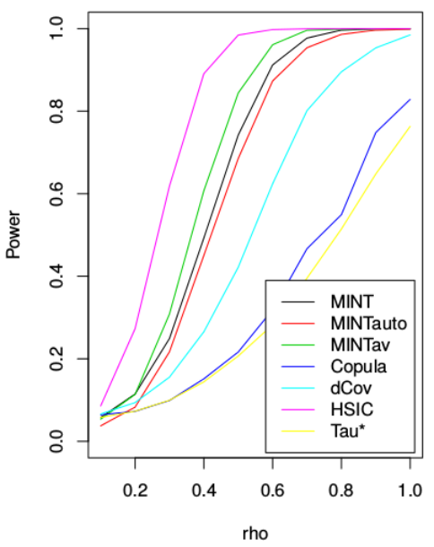
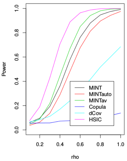
The results are presented in Figure 1. Unsurprisingly, there is no uniformly most powerful test among those considered, and if the form of the dependence were known in advance, it may well be possible to design a tailor-made test with good power. Nevertheless, Figure 1 shows that, especially in the first and second of the three settings described above, the MINT and MINTav approaches have very strong performance. In these examples, the dependence becomes increasingly localised as ll increases, and the flexibility to choose a smaller value of kk in such settings means that MINT approaches are particularly effective. Where the dependence is more global in nature, such as in setting (iii), other approaches may be better suited, though even here, MINT is competitive. Interestingly, the multiscale MINTav appears to be much more effective than the MINTauto approach of choosing a single value of kk; indeed, in setting (iii), MINTav even outperforms the oracle choice of kk.

Refer to caption
Refer to caption
Refer to caption
Refer to caption
Refer to caption
Refer to caption
Figure 1: Power curves for the different tests considered, for settings (i) (left), (ii) (middle) and (iii) (right). The marginals are univariate (top) and bivariate (bottom).

6.3 Real data

In this section we illustrate the use of MINTregression on a data set comprising the average minimum daily January temperature, between 1931 and 1960 and measured in degrees Fahrenheit, in 56 US cities, indexed by their latitude and longitude (Peixoto, 1990). Fitting a normal linear model to the data with temperature as the response and latitude and longitude as covariates leads to the diagnostic plots shown in Figures 2 and 2. Based on these plots, it is relatively difficult to assess the strength of evidence against the model. Centering all of the variables and running MINTregression with kη=6k_{\eta}=6, k=3k=3 and B=1785=⌊105/56⌋B=1785=\lfloor 10^{5}/56\rfloor yielded a pp-value of 0.00224, providing strong evidence that the normal linear model is not a good fit to the data. Further investigation is possible via partial regression: in Figure 2 we plot residuals based on a simple linear fit of Temperature on Latitude against the residuals of another linear fit of Longitude on Latitude. This partial regression plot is indicative of a cubic relationship between Temperature and Longitude after removing the effects of Latitude.

Refer to caption
Refer to caption
Refer to caption
Figure 2: Plots of residuals against fitted values (left) and square roots of the absolute values of the standardised residuals against fitted values (middle) for the US cities temperature data. The right panel gives a partial regression plot after removing the effect of latitude from both the response and longitude.

Based on this evidence we fitted a new model with a quadratic and cubic term in Longitude added to the first model. The pp-value of the resulting FF-test was <2.2×10⁻¹⁶<2.2\times 10^{-16}, giving overwhelming evidence in favour of the inclusion of the quadratic and cubic terms. We then ran our extension of MINTregression to test the independence of ϵ\epsilon and (Longitude,Latitude)(\mathrm{Longitude},\mathrm{Latitude}), as described at the end of Section 5 with B=1000B=1000. This resulted in a pp-value of 0.0679, so we do not reject this model at the 5%5\% significance level.

7 Proofs

7.1 Proofs from Section 3

Proof of Lemma 1.

Under H0H_{0}, the finite sequence (I^n,I^n(1),…,I^n(B))(\widehat{I}_{n},\widehat{I}_{n}^{(1)},\ldots,\widehat{I}_{n}^{(B)}) is exchangeable. If follows that under H0H_{0}, if we split ties at random, then every possible ordering of I^n,I^n(1),…,I^n(B)\widehat{I}_{n},\widehat{I}_{n}^{(1)},\ldots,\widehat{I}_{n}^{(B)} is equally likely. In particular, the (descending order) rank of I^n\widehat{I}_{n} among {I^n,I^n(1),…,I^n(B)}\{\widehat{I}_{n},\widehat{I}_{n}^{(1)},\ldots,\widehat{I}_{n}^{(B)}\}, denoted rank⁡(I^n)\mathrm{rank}(\widehat{I}_{n}), is uniformly distributed on {1,2,…,B+1}\{1,2,\ldots,B+1\}. We deduce that for any k∈{1,…,n−1}k\in\{1,\ldots,n-1\} and writing ℙH0\mathbb{P}_{H_{0}} for the probability under the product of any marginal distributions for XX and YY,

ℙH0​(I^n>C^q(n),B)\displaystyle\mathbb{P}_{H_{0}}\bigl(\widehat{I}_{n}>\widehat{C}_{q}^{(n),B}\bigr) =ℙH0(1B+1∑b=0B𝟙{I^n(b)≥I^n}≤q)\displaystyle=\mathbb{P}_{H_{0}}\biggl(\frac{1}{B+1}\sum_{b=0}^{B}\mathbbm{1}_{\{\widehat{I}_{n}^{(b)}\geq\widehat{I}_{n}\}}\leq q\biggr)
≤ℙH0​(rank⁡(I^n)≤q⁡(B+1))=⌊q⁡(B+1)⌋B+1≤q,\displaystyle\leq\mathbb{P}_{H_{0}}\bigl(\mathrm{rank}(\widehat{I}_{n})\leq q(B+1)\bigr)=\frac{\lfloor q(B+1)\rfloor}{B+1}\leq q,

as required. ∎

Let V⁡(f):=Var​log⁡f⁡(X,Y)fX​(X)​fY​(Y)V(f):=\mathrm{Var}\log\frac{f(X,Y)}{f_{X}(X)f_{Y}(Y)}. The following result will be useful in the proof of Theorem 2.

Lemma 7.

Fix dX,dY∈ℕd_{X},d_{Y}\in\mathbb{N} and ϑ∈Θ2\vartheta\in\Theta^{2}. Then

supf∈ℱdX,dY,ϑ​(0)V⁡(f)I​(f)1/4<∞.\sup_{f\in\mathcal{F}_{d_{X},d_{Y},\vartheta}(0)}\frac{V(f)}{I(f)^{1/4}}<\infty.
Proof of Lemma 7.

For x∈ℝx\in\mathbb{R} we write x−:=max⁡(0,−x)x_{-}:=\max(0,-x). We have

𝔼⁡[{log⁡f⁡(X,Y)fX​(X)​fY​(Y)}−]\displaystyle\mathbb{E}\biggl[\biggl\{\log\frac{f(X,Y)}{f_{X}(X)f_{Y}(Y)}\biggr\}_{-}\biggr] =∫{(x,y):f⁡(x,y)≤fX​(x)​fY​(y)}f(x,y)logfX​(x)​fY​(y)f⁡(x,y)dλd(x,y)\displaystyle=\int_{\{(x,y):f(x,y)\leq f_{X}(x)f_{Y}(y)\}}f(x,y)\log\frac{f_{X}(x)f_{Y}(y)}{f(x,y)}\,d\lambda_{d}(x,y)
≤∫{(x,y):f⁡(x,y)≤fX​(x)​fY​(y)}f(x,y){fX​(x)​fY​(y)f⁡(x,y)−1}dλd(x,y)\displaystyle\leq\int_{\{(x,y):f(x,y)\leq f_{X}(x)f_{Y}(y)\}}f(x,y)\biggl\{\frac{f_{X}(x)f_{Y}(y)}{f(x,y)}-1\biggr\}\,d\lambda_{d}(x,y)
=supA∈ℬ⁡(ℝd){∫AfX​fY−∫Af}≤{I⁡(f)/2}1/2,\displaystyle=\sup_{A\in\mathcal{B}(\mathbb{R}^{d})}\biggl\{\int_{A}f_{X}f_{Y}-\int_{A}f\biggr\}\leq\{I(f)/2\}^{1/2},

where the final inequality is Pinsker’s inequality. We therefore have that

V⁡(f)\displaystyle V(f) ≤𝔼​log2​f⁡(X,Y)fX​(X)​fY​(Y)=𝔼⁡{|log⁡f⁡(X,Y)fX​(X)​fY​(Y)|1/2​|log⁡f⁡(X,Y)fX​(X)​fY​(Y)|3/2}\displaystyle\leq\mathbb{E}\log^{2}\frac{f(X,Y)}{f_{X}(X)f_{Y}(Y)}=\mathbb{E}\biggl\{\Bigl|\log\frac{f(X,Y)}{f_{X}(X)f_{Y}(Y)}\Bigr|^{1/2}\Bigl|\log\frac{f(X,Y)}{f_{X}(X)f_{Y}(Y)}\Bigr|^{3/2}\biggr\}
≤{𝔼​|log⁡f⁡(X,Y)fX​(X)​fY​(Y)|}1/2​{𝔼​|log⁡f⁡(X,Y)fX​(X)​fY​(Y)|3}1/2\displaystyle\leq\biggl\{\mathbb{E}\Bigl|\log\frac{f(X,Y)}{f_{X}(X)f_{Y}(Y)}\Bigr|\biggr\}^{1/2}\biggl\{\mathbb{E}\Bigl|\log\frac{f(X,Y)}{f_{X}(X)f_{Y}(Y)}\Bigr|^{3}\biggr\}^{1/2}
=(I⁡(f)+2​𝔼​[{log⁡f⁡(X,Y)fX​(X)​fY​(Y)}−])1/2​{𝔼​|log⁡f⁡(X,Y)fX​(X)​fY​(Y)|3}1/2\displaystyle=\biggl(I(f)+2\mathbb{E}\biggl[\biggl\{\log\frac{f(X,Y)}{f_{X}(X)f_{Y}(Y)}\biggr\}_{-}\biggr]\biggr)^{1/2}\biggl\{\mathbb{E}\Bigl|\log\frac{f(X,Y)}{f_{X}(X)f_{Y}(Y)}\Bigr|^{3}\biggr\}^{1/2}
≤2​{I⁡(f)+21/2​I​(f)1/2}1/2​{𝔼​|log⁡(fX​(X)​fY​(Y))|3+𝔼​|log⁡f⁡(X,Y)|3}1/2.\displaystyle\leq 2\bigl\{I(f)+2^{1/2}I(f)^{1/2}\bigr\}^{1/2}\bigl\{\mathbb{E}\bigl|\log\bigl(f_{X}(X)f_{Y}(Y)\bigr)\bigr|^{3}+\mathbb{E}|\log f(X,Y)|^{3}\bigr\}^{1/2}.

By Berrett, Samworth and Yuan (2017, Lemma 11(i)), we conclude that

supf∈ℱdX,dY,ϑ:I⁡(f)≤1V⁡(f)I​(f)1/4<∞.\sup_{f\in\mathcal{F}_{d_{X},d_{Y},\vartheta}:I(f)\leq 1}\frac{V(f)}{I(f)^{1/4}}<\infty.

The result follows from this fact, together with the observation that

supf∈ℱdX,dY,ϑV⁡(f)≤2​supf∈ℱdX,dY,ϑ{𝔼​log2⁡f⁡(X,Y)+𝔼​log2⁡(fX​(X)​fY​(Y))}<∞,\sup_{f\in\mathcal{F}_{d_{X},d_{Y},\vartheta}}V(f)\leq 2\sup_{f\in\mathcal{F}_{d_{X},d_{Y},\vartheta}}\bigl\{\mathbb{E}\log^{2}f(X,Y)+\mathbb{E}\log^{2}\bigl(f_{X}(X)f_{Y}(Y)\bigr)\bigr\}<\infty, (7)

where the final bound follows from another application of Berrett, Samworth and Yuan (2017, Lemma 11(i)). ∎

Proof of Theorem 2.

Fix f∈ℱdX,dY,ϑ​(bn)f\in\mathcal{F}_{d_{X},d_{Y},\vartheta}(b_{n}). We have by two applications of Markov’s inequality that

ℙf​(I^n≤C^q(n),Bn)\displaystyle\mathbb{P}_{f}(\widehat{I}_{n}\leq\widehat{C}_{q}^{(n),B_{n}}) ≤1q⁡(Bn+1)​{1+Bn​ℙf​(I^n(1)≥I^n)}\displaystyle\leq\frac{1}{q(B_{n}+1)}\{1+B_{n}\mathbb{P}_{f}(\widehat{I}_{n}^{(1)}\geq\widehat{I}_{n})\}
≤1q​ℙf​(|I^n−I^n(1)−I⁡(f)|≥I⁡(f))+1q⁡(Bn+1)\displaystyle\leq\frac{1}{q}\mathbb{P}_{f}\bigl(|\widehat{I}_{n}-\widehat{I}_{n}^{(1)}-I(f)|\geq I(f)\bigr)+\frac{1}{q(B_{n}+1)}
≤1q​I​(f)2​𝔼f​[{I^n−I^n(1)−I⁡(f)}2]+1q⁡(Bn+1).\displaystyle\leq\frac{1}{qI(f)^{2}}\mathbb{E}_{f}[\{\widehat{I}_{n}-\widehat{I}_{n}^{(1)}-I(f)\}^{2}]+\frac{1}{q(B_{n}+1)}. (8)

It is convenient to define the following entropy estimators based on pseudo-data, as well as oracle versions of our entropy estimators: let Zi(1):=(XiT,Yi(1)​T)TZ_{i}^{(1)}:=(X_{i}^{T},Y_{i}^{(1)T})^{T}, Z(1):=(Z1(1),…,Zn(1))TZ^{(1)}:=(Z_{1}^{(1)},\ldots,Z_{n}^{(1)})^{T} and Y(1):=(Y1(1),…,Yn(1))TY^{(1)}:=(Y_{1}^{(1)},\ldots,Y_{n}^{(1)})^{T} and set

H^nZ,(1):=H^n,kZ,wZ​(Z(1)),\displaystyle\widehat{H}_{n}^{Z,(1)}:=\widehat{H}_{n,k}^{Z,w^{Z}}(Z^{(1)}),\quad H^nY,(1):=H^n,kY,wY​(Y(1))\displaystyle\widehat{H}_{n}^{Y,(1)}:=\widehat{H}_{n,k}^{Y,w^{Y}}(Y^{(1)})
Hn∗:=−1n∑i=1nlogf(Xi,Yi),\displaystyle H_{n}^{*}:=-\frac{1}{n}\sum_{i=1}^{n}\log f(X_{i},Y_{i}),\quad Hn∗,Y:=−1n∑i=1nlogfY(Yi),\displaystyle H_{n}^{*,Y}:=-\frac{1}{n}\sum_{i=1}^{n}\log f_{Y}(Y_{i}),
Hn∗,(1):=−1n∑i=1nlogfX(Xi)fY(Yi(1)),\displaystyle H_{n}^{*,(1)}:=-\frac{1}{n}\sum_{i=1}^{n}\log f_{X}(X_{i})f_{Y}(Y_{i}^{(1)}),\quad Hn∗,Y,(1):=−1n∑i=1nlogfY(Yi(1)).\displaystyle H_{n}^{*,Y,(1)}:=-\frac{1}{n}\sum_{i=1}^{n}\log f_{Y}(Y_{i}^{(1)}).

Writing In∗:=1n​∑i=1nlog⁡f⁡(Xi,Yi)fX​(Xi)​fY​(Yi)I_{n}^{*}:=\frac{1}{n}\sum_{i=1}^{n}\log\frac{f(X_{i},Y_{i})}{f_{X}(X_{i})f_{Y}(Y_{i})} we have by Berrett, Samworth and Yuan (2017, Theorem 1) that

supkY∈{k0∗,…,kY∗}k∈{k0∗,…,k∗}supf∈ℱdX,dY,ϑn​𝔼f​{(I^n−I^n(1)−In∗)2}\displaystyle\sup_{\begin{subarray}{c}k_{Y}\in\{k_{0}^{*},\ldots,k_{Y}^{*}\}\\ k\in\{k_{0}^{*},\ldots,k^{*}\}\end{subarray}}\sup_{f\in\mathcal{F}_{d_{X},d_{Y},\vartheta}}n\mathbb{E}_{f}\{(\widehat{I}_{n}-\widehat{I}_{n}^{(1)}-I_{n}^{*})^{2}\}
=supkY∈{k0∗,…,kY∗}k∈{k0∗,…,k∗}supf∈ℱdX,dY,ϑn​𝔼f​[{H^nY−H^n−H^nY,(1)+H^n(1)−(Hn∗,Y−Hn∗−Hn∗,Y,(1)+Hn∗,(1))}2]\displaystyle=\!\!\!\sup_{\begin{subarray}{c}k_{Y}\in\{k_{0}^{*},\ldots,k_{Y}^{*}\}\\ k\in\{k_{0}^{*},\ldots,k^{*}\}\end{subarray}}\sup_{f\in\mathcal{F}_{d_{X},d_{Y},\vartheta}}\!\!\!\!n\mathbb{E}_{f}\biggl[\biggl\{\widehat{H}_{n}^{Y}-\widehat{H}_{n}-\widehat{H}_{n}^{Y,(1)}+\widehat{H}_{n}^{(1)}-\bigl(H_{n}^{*,Y}-H_{n}^{*}-H_{n}^{*,Y,(1)}+H_{n}^{*,(1)}\bigr)\biggr\}^{2}\biggr]
≤4nsupkY∈{k0∗,…,kY∗}k∈{k0∗,…,k∗}supf∈ℱdX,dY,ϑ𝔼f{(H^nY−Hn∗,Y)2+(H^n−Hn∗)2\displaystyle\leq 4n\sup_{\begin{subarray}{c}k_{Y}\in\{k_{0}^{*},\ldots,k_{Y}^{*}\}\\ k\in\{k_{0}^{*},\ldots,k^{*}\}\end{subarray}}\sup_{f\in\mathcal{F}_{d_{X},d_{Y},\vartheta}}\mathbb{E}_{f}\Bigl\{(\widehat{H}_{n}^{Y}-H_{n}^{*,Y})^{2}+(\widehat{H}_{n}-H_{n}^{*})^{2}
+(H^nY,(1)−Hn∗,Y,(1))2+(H^n(1)−Hn∗,(1))2}→0.\displaystyle\hskip 199.16928pt+(\widehat{H}_{n}^{Y,(1)}-H_{n}^{*,Y,(1)})^{2}+(\widehat{H}_{n}^{(1)}-H_{n}^{*,(1)})^{2}\Bigr\}\rightarrow 0.

It follows by Cauchy–Schwarz and the fact that 𝔼⁡[{In∗−I⁡(f)}2]=V⁡(f)/n\mathbb{E}\bigl[\bigl\{I_{n}^{*}-I(f)\bigr\}^{2}\bigr]=V(f)/n that

ϵn2\displaystyle\epsilon_{n}^{2} :=supkY∈{k0∗,…,kY∗}k∈{k0∗,…,k∗}supf∈ℱdX,dY,ϑ|n​𝔼f​[{I^n−I^n(1)−I⁡(f)}2]−V⁡(f)|\displaystyle:=\sup_{\begin{subarray}{c}k_{Y}\in\{k_{0}^{*},\ldots,k_{Y}^{*}\}\\ k\in\{k_{0}^{*},\ldots,k^{*}\}\end{subarray}}\sup_{f\in\mathcal{F}_{d_{X},d_{Y},\vartheta}}\Bigl|n\mathbb{E}_{f}\bigl[\bigl\{\widehat{I}_{n}-\widehat{I}_{n}^{(1)}-I(f)\bigr\}^{2}\bigr]-V(f)\Bigr|
≤supkY∈{k0∗,…,kY∗}k∈{k0∗,…,k∗}supf∈ℱdX,dY,ϑ{n​𝔼f​{(I^n−I^n(1)−In∗)2}+2​[n​𝔼f​{(I^n−I^n(1)−In∗)2}​V​(f)]1/2}\displaystyle\leq\sup_{\begin{subarray}{c}k_{Y}\in\{k_{0}^{*},\ldots,k_{Y}^{*}\}\\ k\in\{k_{0}^{*},\ldots,k^{*}\}\end{subarray}}\sup_{f\in\mathcal{F}_{d_{X},d_{Y},\vartheta}}\Bigl\{n\mathbb{E}_{f}\{(\widehat{I}_{n}-\widehat{I}_{n}^{(1)}-I_{n}^{*})^{2}\}+2\bigl[n\mathbb{E}_{f}\{(\widehat{I}_{n}-\widehat{I}_{n}^{(1)}-I_{n}^{*})^{2}\}V(f)\bigr]^{1/2}\Bigr\}
→0,\displaystyle\rightarrow 0, (9)

where we use (7) to bound V⁡(f)V(f) above. Now consider bn:=max(ϵn1/2n−1/2,n−4/7logn)b_{n}:=\max(\epsilon_{n}^{1/2}n^{-1/2},n^{-4/7}\log n). By (8), (9) and Lemma 7 we have that

infBn≥Bn∗infkY∈{k0∗,…,kY∗}k∈{k0∗,…,k∗}\displaystyle\inf_{B_{n}\geq B_{n}^{*}}\inf_{\begin{subarray}{c}k_{Y}\in\{k_{0}^{*},\ldots,k_{Y}^{*}\}\\ k\in\{k_{0}^{*},\ldots,k^{*}\}\end{subarray}} inff∈ℱdX,dY,ϑ​(bn)ℙf​(I^n>Cq(n),Bn)\displaystyle\inf_{f\in\mathcal{F}_{d_{X},d_{Y},\vartheta}(b_{n})}\mathbb{P}_{f}(\widehat{I}_{n}>C_{q}^{(n),B_{n}})
≥1−supkY∈{k0∗,…,kY∗}k∈{k0∗,…,k∗}supf∈ℱdX,dY,ϑ​(bn)𝔼⁡[{I^n−I^n(1)−I⁡(f)}2]q​I​(f)2−1q⁡(Bn∗+1)\displaystyle\geq 1-\sup_{\begin{subarray}{c}k_{Y}\in\{k_{0}^{*},\ldots,k_{Y}^{*}\}\\ k\in\{k_{0}^{*},\ldots,k^{*}\}\end{subarray}}\sup_{f\in\mathcal{F}_{d_{X},d_{Y},\vartheta}(b_{n})}\frac{\mathbb{E}[\{\widehat{I}_{n}-\widehat{I}_{n}^{(1)}-I(f)\}^{2}]}{qI(f)^{2}}-\frac{1}{q(B_{n}^{*}+1)}
≥1−supf∈ℱdX,dY,ϑ​(bn)V⁡(f)+ϵn2n​q​I​(f)2−1q⁡(Bn∗+1)\displaystyle\geq 1-\sup_{f\in\mathcal{F}_{d_{X},d_{Y},\vartheta}(b_{n})}\frac{V(f)+\epsilon_{n}^{2}}{nqI(f)^{2}}-\frac{1}{q(B_{n}^{*}+1)}
≥1−1q​log7/4​n​supf∈ℱdX,dY,ϑ​(0)V⁡(f)I​(f)1/4−ϵnq−1q⁡(Bn∗+1)→1,\displaystyle\geq 1-\frac{1}{q\log^{7/4}n}\sup_{f\in\mathcal{F}_{d_{X},d_{Y},\vartheta}(0)}\frac{V(f)}{I(f)^{1/4}}-\frac{\epsilon_{n}}{q}-\frac{1}{q(B_{n}^{*}+1)}\rightarrow 1,

as required. ∎

7.2 Proofs from Section 4

Proof of Lemma 3.

We first claim that (I^n(0),I^n(1),…,I^n(B))(\widehat{I}_{n}^{(0)},\widehat{I}_{n}^{(1)},\ldots,\widehat{I}_{n}^{(B)}) is an exchangeable sequence under H0H_{0}. Indeed, let σ\sigma be an arbitrary permutation of {0,1,…,B}\{0,1,\ldots,B\}, and recall that I^n(b)\widehat{I}_{n}^{(b)} is computed from (Xi,Yτb​(i))i=1n(X_{i},Y_{\tau_{b}(i)})_{i=1}^{n}, where τb\tau_{b} is uniformly distributed on SnS_{n}. Note that, under H0H_{0}, we have (Xi,Yi)i=1n​=𝑑​(Xi,Yτ⁡(i))i=1n(X_{i},Y_{i})_{i=1}^{n}\overset{d}{=}(X_{i},Y_{\tau(i)})_{i=1}^{n} for any τ∈Sn\tau\in S_{n}. Hence, for any A∈ℬ⁡(ℝB+1)A\in\mathcal{B}(\mathbb{R}^{B+1}),

ℙH0​((I^n(σ⁡(0)),…,I^n(σ⁡(B)))∈A)\displaystyle\mathbb{P}_{H_{0}}\bigl((\widehat{I}_{n}^{(\sigma(0))},\ldots,\widehat{I}_{n}^{(\sigma(B))})\in A\bigr)
=1(n!)B​∑π1,…,πB∈SnℙH0​((I^n(σ⁡(0)),…,I^n(σ⁡(B)))∈A|τ1=π1,…,τB=πB)\displaystyle=\frac{1}{(n!)^{B}}\sum_{\pi_{1},\ldots,\pi_{B}\in S_{n}}\mathbb{P}_{H_{0}}\bigl((\widehat{I}_{n}^{(\sigma(0))},\ldots,\widehat{I}_{n}^{(\sigma(B))})\in A|\tau_{1}=\pi_{1},\ldots,\tau_{B}=\pi_{B}\bigr)
=1(n!)B​∑π1,…,πB∈SnℙH0​((I^n(0),…,I^n(B))∈A|τ1=πσ⁡(1)​πσ⁡(0)−1,…,τB=πσ⁡(B)​πσ⁡(0)−1)\displaystyle=\frac{1}{(n!)^{B}}\sum_{\pi_{1},\ldots,\pi_{B}\in S_{n}}\mathbb{P}_{H_{0}}\bigl((\widehat{I}_{n}^{(0)},\ldots,\widehat{I}_{n}^{(B)})\in A|\tau_{1}=\pi_{\sigma(1)}\pi_{\sigma(0)}^{-1},\ldots,\tau_{B}=\pi_{\sigma(B)}\pi_{\sigma(0)}^{-1}\bigr)
=ℙH0​((I^n(0),…,I^n(B))∈A).\displaystyle=\mathbb{P}_{H_{0}}\bigl((\widehat{I}_{n}^{(0)},\ldots,\widehat{I}_{n}^{(B)})\in A\bigr).

By the same argument as in the proof of Lemma 1 we now have that

ℙH0​(I^n>C~q(n),B)≤⌊q⁡(B+1)⌋B+1≤q,\mathbb{P}_{H_{0}}(\widehat{I}_{n}>\tilde{C}_{q}^{(n),B})\leq\frac{\lfloor q(B+1)\rfloor}{B+1}\leq q,

as required. ∎

Recall the definition of H^n(1)\widehat{H}_{n}^{(1)} given just after (3). We give the proof of Theorem 4 below, followed by Lemma 8, which is the key ingredient on which it is based.

Proof of Theorem 4.

We have by Markov’s inequality that

ℙf​(I^n≤C~q(n),Bn)\displaystyle\mathbb{P}_{f}(\widehat{I}_{n}\leq\tilde{C}_{q}^{(n),B_{n}}) ≤1q⁡(Bn+1)​{1+Bn​ℙf​(I^n≤I~n(1))}≤1q​ℙf​(H^nZ≥H~n(1))+1q⁡(Bn+1).\displaystyle\leq\frac{1}{q(B_{n}+1)}\{1+B_{n}\mathbb{P}_{f}(\widehat{I}_{n}\leq\tilde{I}_{n}^{(1)})\}\leq\frac{1}{q}\mathbb{P}_{f}(\widehat{H}_{n}^{Z}\geq\tilde{H}_{n}^{(1)})+\frac{1}{q(B_{n}+1)}. (10)

But

ℙf​(H^nZCLOSE\displaystyle\mathbb{P}_{f}(\widehat{H}_{n}^{Z} OPEN≥H^n(1))=ℙf​(H^nZ−H⁡(X,Y)≥H^n(1)−H⁡(X)−H⁡(Y)+I⁡(X,Y))\displaystyle\geq\widehat{H}_{n}^{(1)})=\mathbb{P}_{f}\bigl(\widehat{H}_{n}^{Z}-H(X,Y)\geq\widehat{H}_{n}^{(1)}-H(X)-H(Y)+I(X;Y)\bigr)
≤ℙ⁡(|H^nZ−H⁡(X,Y)|≥12​I​(X,Y))+ℙ⁡(|H^n(1)−H⁡(X)−H⁡(Y)|≥12​I​(X,Y))\displaystyle\leq\mathbb{P}\Bigl(|\widehat{H}_{n}^{Z}-H(X,Y)|\geq\frac{1}{2}I(X;Y)\Bigr)+\mathbb{P}\Bigl(|\widehat{H}_{n}^{(1)}-H(X)-H(Y)|\geq\frac{1}{2}I(X;Y)\Bigr)
≤2I⁡(X,Y)​{𝔼​|H^nZ−H⁡(X,Y)​|+𝔼|​H^n(1)−H⁡(X)−H⁡(Y)|}.\displaystyle\leq\frac{2}{I(X;Y)}\bigl\{\mathbb{E}|\widehat{H}_{n}^{Z}-H(X,Y)|+\mathbb{E}|\widehat{H}_{n}^{(1)}-H(X)-H(Y)|\bigr\}. (11)

The theorem therefore follows immediately from (10), (11) and Lemma 8 below. ∎

Lemma 8.

Let dX,dY∈ℕd_{X},d_{Y}\in\mathbb{N}, let d=dX+dYd=d_{X}+d_{Y} and fix ϕ=(α,μ,ν,(cn),(pn))∈Φ\phi=(\alpha,\mu,\nu,(c_{n}),(p_{n}))\in\Phi with cn→0c_{n}\rightarrow 0 and pn=o⁡(1/log⁡n)p_{n}=o(1/\log n) as n→∞n\rightarrow\infty. Let k0∗=k0,n∗k_{0}^{*}=k_{0,n}^{*} and k1∗=k1,n∗k_{1}^{*}=k_{1,n}^{*} denote two deterministic sequences of positive integers satisfying k0∗≤k1∗k_{0}^{*}\leq k_{1}^{*}, k0∗/log2⁡n→∞k_{0}^{*}/\log^{2}n\rightarrow\infty and (k1∗​log2​n)/n→0(k_{1}^{*}\log^{2}n)/n\rightarrow 0. Then

supk∈{k0∗,…,k1∗}supf∈𝒢dX,dY,ϕ\displaystyle\sup_{k\in\{k_{0}^{*},\ldots,k_{1}^{*}\}}\sup_{f\in\mathcal{G}_{d_{X},d_{Y},\phi}} 𝔼f​|H^n(1)−H⁡(X)−H⁡(Y)|→0,\displaystyle\mathbb{E}_{f}|\widehat{H}_{n}^{(1)}-H(X)-H(Y)|\rightarrow 0,
supk∈{k0∗,…,k1∗}supf∈ℋd,ϕ\displaystyle\sup_{k\in\{k_{0}^{*},\ldots,k_{1}^{*}\}}\sup_{f\in\mathcal{H}_{d,\phi}} 𝔼f​|H^nZ−H⁡(X,Y)|→0\displaystyle\mathbb{E}_{f}|\widehat{H}_{n}^{Z}-H(X,Y)|\rightarrow 0

as n→∞n\rightarrow\infty.

Proof.

We prove only the first claim in Lemma 8, since the second claim involves similar arguments but is more straightforward because the estimator is based on an independent and identically distributed sample and no permutations are involved. Throughout this proof, we write a≲ba\lesssim b to mean that there exists C>0C>0, depending only on dX,dY∈ℕd_{X},d_{Y}\in\mathbb{N} and ϕ∈Φ\phi\in\Phi, such that a≤C​ba\leq Cb. Fix f∈𝒢dX,dY,ϕf\in\mathcal{G}_{d_{X},d_{Y},\phi}, where ϕ=(α,μ,ν,(cn),(pn))\phi=(\alpha,\mu,\nu,(c_{n}),(p_{n})). Write ρ(k),i,(1)\rho_{(k),i,(1)} for the distance from Zi(1)Z_{i}^{(1)} to its kkth nearest neighbour in the sample Z1(1),…,Zn(1)Z_{1}^{(1)},\ldots,Z_{n}^{(1)} and ξi(1):=e−Ψ⁡(k)​Vd​(n−1)​ρ(k),i,(1)d\xi_{i}^{(1)}:=e^{-\Psi(k)}V_{d}(n-1)\rho_{(k),i,(1)}^{d} so that

H^n(1)=1n​∑i=1nlog⁡ξi(1).\widehat{H}_{n}^{(1)}=\frac{1}{n}\sum_{i=1}^{n}\log\xi_{i}^{(1)}.

Recall that SnS_{n} denotes the set of all permutations of {1,…,n}\{1,\ldots,n\}, and define Snl⊆SnS_{n}^{l}\subseteq S_{n} to be the set of permutations that fix {1,…,l}\{1,\ldots,l\} and have no fixed points among {l+1,…,n}\{l+1,\ldots,n\}; thus |Snl|=(n−l)!​∑r=0n−l(−1)r/r!|S_{n}^{l}|=(n-l)!\sum_{r=0}^{n-l}(-1)^{r}/r!. For τ∈Sn\tau\in S_{n}, write ℙτ(⋅):=ℙ(⋅|τ1=τ)\mathbb{P}_{\tau}(\cdot):=\mathbb{P}(\cdot|\tau_{1}=\tau), and 𝔼τ(⋅):=𝔼(⋅|τ1=τ)\mathbb{E}_{\tau}(\cdot):=\mathbb{E}(\cdot|\tau_{1}=\tau). Let ln:=⌊log⁡log⁡n⌋l_{n}:=\lfloor\log\log n\rfloor. For i=1,…,ni=1,\ldots,n, let

Ai′:={The k nearest neighbours of Zi(1) are among Zl+1(1),…,Zn(1)},A^{\prime}_{i}:=\{\text{The $k$ nearest neighbours of $Z_{i}^{(1)}$ are among $Z_{l+1}^{(1)},\ldots,Z_{n}^{(1)}$}\},

and let Ai:=Ai′∩{Zi(1)∈𝒲n}A_{i}:=A^{\prime}_{i}\cap\{Z_{i}^{(1)}\in\mathcal{W}_{n}\}. Using the exchangeability of ξ1(1),…,ξn(1)\xi_{1}^{(1)},\ldots,\xi_{n}^{(1)}, our basic decomposition is as follows:

𝔼​|H^n(1)−H⁡(X)−H⁡(Y)|\displaystyle\mathbb{E}\bigl|\widehat{H}_{n}^{(1)}-H(X)-H(Y)|
≤1n!​∑l=0ln(nl)​∑τ∈Snl{1n​∑i=1l𝔼τ​|log⁡ξi(1)​|+𝔼τ|​1n​∑i=l+1nlog⁡ξi(1)−H⁡(X)−H⁡(Y)|}\displaystyle\leq\frac{1}{n!}\sum_{l=0}^{l_{n}}\binom{n}{l}\sum_{\tau\in S_{n}^{l}}\biggl\{\frac{1}{n}\sum_{i=1}^{l}\mathbb{E}_{\tau}|\log\xi_{i}^{(1)}|+\mathbb{E}_{\tau}\biggl|\frac{1}{n}\sum_{i=l+1}^{n}\log\xi_{i}^{(1)}-H(X)-H(Y)\biggr|\biggr\}
+1n!∑l=ln+1n(nl)∑τ∈Snl𝔼τ|H^n(1)−H(X)−H(Y)|\displaystyle\hskip 199.16928pt+\frac{1}{n!}\sum_{l=l_{n}+1}^{n}\binom{n}{l}\sum_{\tau\in S_{n}^{l}}\mathbb{E}_{\tau}\bigl|\widehat{H}_{n}^{(1)}-H(X)-H(Y)\bigr|
≤1n!∑l=0ln(nl)∑τ∈Snl{1n∑i=1l𝔼τ|logξi(1)|+𝔼τ|1n∑i=l+1n(logξi(1))𝟙Ai−H(X)−H(Y)|\displaystyle\leq\frac{1}{n!}\sum_{l=0}^{l_{n}}\binom{n}{l}\sum_{\tau\in S_{n}^{l}}\biggl\{\frac{1}{n}\sum_{i=1}^{l}\mathbb{E}_{\tau}|\log\xi_{i}^{(1)}|+\mathbb{E}_{\tau}\biggl|\frac{1}{n}\sum_{i=l+1}^{n}(\log\xi_{i}^{(1)})\mathbbm{1}_{A_{i}}-H(X)-H(Y)\biggr|
+1n∑i=l+1n𝔼τ(|logξi(1)|𝟙{(Aic∖(Ai′)c)∪(Ai′)c})}+1n!∑l=ln+1n(nl)∑τ∈Snl𝔼τ(|H^n(1)|+|H(X)+H(Y)|).\displaystyle+\frac{1}{n}\sum_{i=l+1}^{n}\mathbb{E}_{\tau}\bigl(|\log\xi_{i}^{(1)}|\mathbbm{1}_{\{(A_{i}^{c}\setminus(A_{i}^{\prime})^{c})\cup(A_{i}^{\prime})^{c}\}}\bigr)\biggr\}+\frac{1}{n!}\sum_{l=l_{n}+1}^{n}\binom{n}{l}\sum_{\tau\in S_{n}^{l}}\mathbb{E}_{\tau}\bigl(|\widehat{H}_{n}^{(1)}|+|H(X)+H(Y)|\bigr). (12)

The rest of the proof consists of handling each of these four terms.

Step 1: We first show that

supk∈{1,…,n−1}supf∈𝒢dX,dY,ϕ1n!​∑l=ln+1n(nl)​∑τ∈Snl𝔼τ​(|H^n(1)|+|H⁡(X)+H⁡(Y)|)→0\sup_{k\in\{1,\ldots,n-1\}}\sup_{f\in\mathcal{G}_{d_{X},d_{Y},\phi}}\frac{1}{n!}\sum_{l=l_{n}+1}^{n}\binom{n}{l}\sum_{\tau\in S_{n}^{l}}\mathbb{E}_{\tau}\bigl(|\widehat{H}_{n}^{(1)}|+|H(X)+H(Y)|\bigr)\rightarrow 0 (13)

as n→∞n\rightarrow\infty. Writing ρ(k),i,X\rho_{(k),i,X} for the distance from XiX_{i} to its kkth nearest neighbour in the sample X1,…,XnX_{1},\ldots,X_{n} and defining ρ(k),i,Y\rho_{(k),i,Y} similarly, we have

max⁡{ρ(k),i,X2,ρ(k),τ1​(i),Y2}≤ρ(k),i,(1)2≤ρ(n−1),i,X2+ρ(n−1),τ1​(i),Y2.\max\{\rho_{(k),i,X}^{2},\rho_{(k),\tau_{1}(i),Y}^{2}\}\leq\rho_{(k),i,(1)}^{2}\leq\rho_{(n-1),i,X}^{2}+\rho_{(n-1),\tau_{1}(i),Y}^{2}.

Using the fact that log⁡(a+b)≤log⁡2+|log⁡a|+|log⁡b|\log(a+b)\leq\log 2+|\log a|+|\log b| for a,b>0a,b>0, we therefore have that

|\displaystyle| log⁡ξi(1)|≤|log⁡(Vd​(n−1)eΨ⁡(k))​|+d|​log⁡ρ(k),i,X|+d2​log⁡(ρ(k),i,(1)2ρ(k),i,X2)\displaystyle\log\xi_{i}^{(1)}|\leq\biggl|\log\biggl(\frac{V_{d}(n-1)}{e^{\Psi(k)}}\biggr)\biggr|+d|\log\rho_{(k),i,X}|+\frac{d}{2}\log\biggl(\frac{\rho_{(k),i,(1)}^{2}}{\rho_{(k),i,X}^{2}}\biggr)
≤|log⁡(Vd​(n−1)eΨ⁡(k))|+2​d|log⁡ρ(k),i,X​|+d2​log​2+d|​log​ρ(n−1),i,X|+d​|log⁡ρ(n−1),τ1​(i),Y|\displaystyle\leq\biggl|\log\biggl(\frac{V_{d}(n-1)}{e^{\Psi(k)}}\biggr)\biggr|+2d|\log\rho_{(k),i,X}|+\frac{d}{2}\log 2+d|\log\rho_{(n-1),i,X}|+d|\log\rho_{(n-1),\tau_{1}(i),Y}| (14)
≤|log⁡(Vd​(n−1)eΨ⁡(k))|+d2​log⁡2\displaystyle\leq\biggl|\log\biggl(\frac{V_{d}(n-1)}{e^{\Psi(k)}}\biggr)\biggr|+\frac{d}{2}\log 2
+4​d​maxj=1,…,n​max⁡{−log⁡ρ(1),j,X,−log⁡ρ(1),j,Y,log⁡ρ(n−1),j,X,log⁡ρ(n−1),j,Y}.\displaystyle\hskip 28.45274pt+4d\max_{j=1,\ldots,n}\max\{-\log\rho_{(1),j,X}\,,\,-\log\rho_{(1),j,Y}\,,\,\log\rho_{(n-1),j,X}\,,\,\log\rho_{(n-1),j,Y}\}. (15)

Now, by the triangle inequality, a union bound and Markov’s inequality,

𝔼{maxj=1,…,n\displaystyle\mathbb{E}\Bigl\{\max_{j=1,\ldots,n} logρ(n−1),j,X}−log2≤𝔼log(maxj=1,…,n∥Xj∥)≤𝔼[{log(maxj=1,…,n∥Xj∥)}+]\displaystyle\log\rho_{(n-1),j,X}\Bigr\}-\log 2\leq\mathbb{E}\log\Bigl(\max_{j=1,\ldots,n}\|X_{j}\|\Bigr)\leq\mathbb{E}\Bigl[\Bigl\{\log\Bigl(\max_{j=1,\ldots,n}\|X_{j}\|\Bigr)\Bigr\}_{+}\Bigr]
=∫0∞ℙ⁡(maxj=1,…,n⁡‖Xj‖≥eM)​𝑑M\displaystyle=\int_{0}^{\infty}\mathbb{P}\Bigl(\max_{j=1,\ldots,n}\|X_{j}\|\geq e^{M}\Bigr)\,dM
≤1α​max​{0,log⁡n+log⁡𝔼⁡(‖X1‖α)}+1α​n​𝔼​(‖X1‖α)​exp​{−log⁡n−log⁡𝔼⁡(‖X1‖α)}\displaystyle\leq\frac{1}{\alpha}\max\bigl\{0,\log n+\log\mathbb{E}(\|X_{1}\|^{\alpha})\bigr\}+\frac{1}{\alpha}n\mathbb{E}(\|X_{1}\|^{\alpha})\exp\bigl\{-\log n-\log\mathbb{E}(\|X_{1}\|^{\alpha})\bigr\}
≤1α​{1+log⁡n+max⁡(0,log⁡μ)},\displaystyle\leq\frac{1}{\alpha}\bigl\{1+\log n+\max(0,\log\mu)\bigr\}, (16)

and the same bound holds for 𝔼​maxj=1,…,n​log⁡ρ(n−1),j,Y\mathbb{E}\max_{j=1,\ldots,n}\log\rho_{(n-1),j,Y}. Similarly,

𝔼⁡[{minj=1,…,n⁡log⁡ρ(1),j,X}−]\displaystyle\mathbb{E}\Bigl[\Bigl\{\min_{j=1,\ldots,n}\log\rho_{(1),j,X}\Bigr\}_{-}\Bigr] =∫0∞ℙ⁡(minj=1,…,n⁡ρ(1),j,X≤e−M)​𝑑M\displaystyle=\int_{0}^{\infty}\mathbb{P}\Bigl(\min_{j=1,\ldots,n}\rho_{(1),j,X}\leq e^{-M}\Bigr)\,dM
≤2​dX−1​log⁡n+n⁡(n−1)​VdX|fX|∫2​dX−1​log⁡n∞∞⁡e−M​dX​𝑑M\displaystyle\leq 2d_{X}^{-1}\log n+n(n-1)V_{d_{X}}\|f_{X}\|_{\infty}\int_{2d_{X}^{-1}\log n}^{\infty}e^{-Md_{X}}\,dM
≤2​dX−1​log⁡n+dX−1​VdX​ν,\displaystyle\leq 2d_{X}^{-1}\log n+d_{X}^{-1}V_{d_{X}}\nu, (17)

and the same bound holds for 𝔼⁡[{minj=1,…,n⁡log⁡ρ(1),j,Y}−]\mathbb{E}\bigl[\bigl\{\min_{j=1,\ldots,n}\log\rho_{(1),j,Y}\bigr\}_{-}\bigr] once we replace dXd_{X} with dYd_{Y}. By (15), (16), (17) and Stirling’s approximation,

∑l=ln+1n\displaystyle\sum_{l=l_{n}+1}^{n} (nl)maxk=1,…,n−1supf∈𝒢dX,dY,ϕ𝔼(|H^n(1)|𝟙{τ1∈Snl})≲logn∑l=ln+1n(nl)ℙ(τ1∈Snl)\displaystyle\binom{n}{l}\max_{k=1,\ldots,n-1}\sup_{f\in\mathcal{G}_{d_{X},d_{Y},\phi}}\mathbb{E}(|\widehat{H}_{n}^{(1)}|\mathbbm{1}_{\{\tau_{1}\in S_{n}^{l}\}})\lesssim\log n\sum_{l=l_{n}+1}^{n}\binom{n}{l}\mathbb{P}(\tau_{1}\in S_{n}^{l})
≤log⁡nn!​(nln+1)​(n−ln−1)!=log⁡n(ln+1)!≤log⁡n2​π​(ln+1)​(eln+1)ln+1→0\displaystyle\leq\frac{\log n}{n!}\binom{n}{l_{n}+1}(n-l_{n}-1)!=\frac{\log n}{(l_{n}+1)!}\leq\frac{\log n}{\sqrt{2\pi(l_{n}+1)}}\biggl(\frac{e}{l_{n}+1}\biggr)^{l_{n}+1}\rightarrow 0 (18)

as n→∞n\rightarrow\infty. Moreover, for any f∈𝒢dX,dY,ϕf\in\mathcal{G}_{d_{X},d_{Y},\phi} and (X,Y)∼f(X,Y)\sim f, writing ϵ=α/(α+2​dX)\epsilon=\alpha/(\alpha+2d_{X}),

|H⁡(X)|≤∫𝒳fX​|log⁡fX|\displaystyle|H(X)|\leq\int_{\mathcal{X}}f_{X}|\log f_{X}| ≤∫𝒳fX​(x)​log⁡(‖fX‖∞fX​(x))​𝑑x+|log⁡‖fX‖∞|\displaystyle\leq\int_{\mathcal{X}}f_{X}(x)\log\biggl(\frac{\|f_{X}\|_{\infty}}{f_{X}(x)}\biggr)\,dx+|\log\|f_{X}\|_{\infty}|
≤‖fX‖∞ϵϵ​∫𝒳fX​(x)1−ϵ​𝑑x+|log⁡‖fX‖∞|\displaystyle\leq\frac{\|f_{X}\|_{\infty}^{\epsilon}}{\epsilon}\int_{\mathcal{X}}f_{X}(x)^{1-\epsilon}\,dx+|\log\|f_{X}\|_{\infty}|
≤νϵϵ​(1+μ)1−ϵ​{∫ℝdX(1+‖x‖α)−1−ϵϵ​𝑑x}ϵ\displaystyle\leq\frac{\nu^{\epsilon}}{\epsilon}(1+\mu)^{1-\epsilon}\biggl\{\int_{\mathbb{R}^{d_{X}}}(1+\|x\|^{\alpha})^{-\frac{1-\epsilon}{\epsilon}}\,dx\biggr\}^{\epsilon}
+max⁡{log⁡ν,1α​log⁡(VdXα​μdX​(α+dX)α+dXαα​dXdX)},\displaystyle\hskip 42.67912pt+\max\biggl\{\log\nu\,,\,\frac{1}{\alpha}\log\biggl(\frac{V_{d_{X}}^{\alpha}\mu^{d_{X}}(\alpha+d_{X})^{\alpha+d_{X}}}{\alpha^{\alpha}d_{X}^{d_{X}}}\biggr)\biggr\}, (19)

where the lower bound on ‖fX‖∞\|f_{X}\|_{\infty} is due to the fact that VdXα​μα​(fX)dX​‖fX‖∞α≥αα​dXdX/(α+dX)α+dXV_{d_{X}}^{\alpha}\mu_{\alpha}(f_{X})^{d_{X}}\|f_{X}\|_{\infty}^{\alpha}\geq\alpha^{\alpha}d_{X}^{d_{X}}/(\alpha+d_{X})^{\alpha+d_{X}} by Berrett, Samworth and Yuan (2017, Lemma 10(i)). Combining (19) with the corresponding bound on H⁡(Y)H(Y), as well as (18), we deduce that (13) holds.

Step 2: We observe that by (15), (16) and (17),

supk∈{1,…,n−1}supf∈𝒢dX,dY,ϕ1n!​∑l=0ln(nl)​∑τ∈Snl1n​∑i=1l𝔼τ​|log⁡ξi(1)|≲ln​log⁡nn→0.\sup_{k\in\{1,\ldots,n-1\}}\sup_{f\in\mathcal{G}_{d_{X},d_{Y},\phi}}\frac{1}{n!}\sum_{l=0}^{l_{n}}\binom{n}{l}\sum_{\tau\in S_{n}^{l}}\frac{1}{n}\sum_{i=1}^{l}\mathbb{E}_{\tau}|\log\xi_{i}^{(1)}|\lesssim\frac{l_{n}\log n}{n}\rightarrow 0. (20)

Step 3: We now show that

supk∈{k0∗,…,k1∗}supf∈𝒢dX,dY,ϕ1n!​∑l=0ln(nl)​∑τ∈Snl1n​∑i=l+1n𝔼τ​(|log⁡ξi(1)|​𝟙{(Aic∖(Ai′)c)∪(Ai′)c})→0.\sup_{k\in\{k_{0}^{*},\ldots,k_{1}^{*}\}}\sup_{f\in\mathcal{G}_{d_{X},d_{Y},\phi}}\frac{1}{n!}\sum_{l=0}^{l_{n}}\binom{n}{l}\sum_{\tau\in S_{n}^{l}}\frac{1}{n}\sum_{i=l+1}^{n}\mathbb{E}_{\tau}\bigl(|\log\xi_{i}^{(1)}|\mathbbm{1}_{\{(A_{i}^{c}\setminus(A_{i}^{\prime})^{c})\cup(A_{i}^{\prime})^{c}\}}\bigr)\rightarrow 0. (21)

We use an argument that involves covering ℝd\mathbb{R}^{d} by cones; cf. Biau and Devroye (2015, Section 20.7). For w0∈ℝdw_{0}\in\mathbb{R}^{d}, z∈ℝd∖{0}z\in\mathbb{R}^{d}\setminus\{0\} and θ∈[0,π]\theta\in[0,\pi], define the cone of angle θ\theta centred at w0w_{0} in the direction zz by

𝒞⁡(w0,z,θ):=w0+{w∈ℝd∖{0}:cos−1⁡(zT​w/(‖z‖​‖w‖))≤θ}∪{0}.\mathcal{C}(w_{0},z,\theta):=w_{0}+\bigl\{w\in\mathbb{R}^{d}\setminus\{0\}:\cos^{-1}(z^{T}w/(\|z\|\|w\|))\leq\theta\bigr\}\cup\{0\}.

By Biau and Devroye (2015, Theorem 20.15), there exists a constant Cπ/6∈ℕC_{\pi/6}\in\mathbb{N} depending only on dd such that we may cover ℝd\mathbb{R}^{d} by Cπ/6C_{\pi/6} cones of angle π/6\pi/6 centred at Z1(1)Z_{1}^{(1)}. In each cone, mark the kk nearest points to Z1(1)Z_{1}^{(1)} among Z2(1),…,Zn(1)Z_{2}^{(1)},\ldots,Z_{n}^{(1)}. Now fix a point Zi(1)Z_{i}^{(1)} that is not marked and a cone that contains it, and let Zi1(1),…,Zik(1)Z_{i_{1}}^{(1)},\ldots,Z_{i_{k}}^{(1)} be the kk marked points in this cone. By Biau and Devroye (2015, Lemma 20.5) we have, for each j=1,…,kj=1,\ldots,k, that

‖Zi(1)−Zij(1)‖<‖Zi(1)−Z1(1)‖.\|Z_{i}^{(1)}-Z_{i_{j}}^{(1)}\|<\|Z_{i}^{(1)}-Z_{1}^{(1)}\|.

Thus, Z1(1)Z_{1}^{(1)} is not one of the kk nearest neighbours of the unmarked point Zi(1)Z_{i}^{(1)}, and only the marked points, of which there are at most k​Cπ/6kC_{\pi/6}, may have Z1(1)Z_{1}^{(1)} as one of their kk nearest neighbours. This immediately generalises to show that at most k​l​Cπ/6klC_{\pi/6} of the points Zl+1(1),…,Zn(1)Z_{l+1}^{(1)},\ldots,Z_{n}^{(1)} may have any of Z1(1),…,Zl(1)Z_{1}^{(1)},\ldots,Z_{l}^{(1)} among their kk nearest neighbours. Then, by (15), (16) and (17), we have that, uniformly over k∈{1,…,n−1}k\in\{1,\ldots,n-1\},

supf∈𝒢dX,dY,ϕmaxτ∈∪l=0lnSnl1n𝔼τ(∑i=l+1n|logξi(1)|𝟙(Ai′)c)≲k​lnnlogn.\sup_{f\in\mathcal{G}_{d_{X},d_{Y},\phi}}\max_{\tau\in\cup_{l=0}^{l_{n}}S_{n}^{l}}\frac{1}{n}\mathbb{E}_{\tau}\biggl(\sum_{i=l+1}^{n}|\log\xi_{i}^{(1)}|\mathbbm{1}_{(A^{\prime}_{i})^{c}}\biggr)\lesssim\frac{kl_{n}}{n}\log n. (22)

Now, for x∈𝒳x\in\mathcal{X} and r∈[0,∞)r\in[0,\infty), let hx​(r):=∫Bx​(r)fXh_{x}(r):=\int_{B_{x}(r)}f_{X}, and, for s∈[0,1)s\in[0,1), let hx−1​(s):=inf{r≥0:hx​(r)≥s}h_{x}^{-1}(s):=\inf\{r\geq 0:h_{x}(r)\geq s\}. We also write Bk,n−k​(s):=Γ⁡(n)Γ⁡(k)​Γ​(n−k)​sk−1​(1−s)n−k−1\mathrm{B}_{k,n-k}(s):=\frac{\Gamma(n)}{\Gamma(k)\Gamma(n-k)}s^{k-1}(1-s)^{n-k-1} for s∈(0,1)s\in(0,1). Then, by (4) and (13) in Berrett, Samworth and Yuan (2017), there exists C>0C>0, depending only on dXd_{X} and ϕ\phi, such that, uniformly for k∈{1,…,n−1}k\in\{1,\ldots,n-1\},

maxi=l+1,…,n𝔼τ{|logρ(k),i,X|𝟙{Zi(1)∈𝒲nc}}\displaystyle\max_{i=l+1,\ldots,n}\mathbb{E}_{\tau}\bigl\{|\log\rho_{(k),i,X}|\mathbbm{1}_{\{Z_{i}^{(1)}\in\mathcal{W}_{n}^{c}\}}\bigr\}
=∫𝒲ncfX​(x)​fY​(y)​∫01|log⁡(VdX​(n−1)​hx−1​(s)eΨ⁡(k))|​Bk,n−k​(s)​𝑑s​d​λd​(x,y)\displaystyle=\int_{\mathcal{W}_{n}^{c}}f_{X}(x)f_{Y}(y)\int_{0}^{1}\biggl|\log\biggl(\frac{V_{d_{X}}(n-1)h_{x}^{-1}(s)}{e^{\Psi(k)}}\biggr)\biggr|\mathrm{B}_{k,n-k}(s)\,ds\,d\lambda_{d}(x,y)
≲∫𝒲ncfX​(x)​fY​(y)​∫01{log⁡n−log⁡s−log⁡(1−s)+log⁡(1+C​‖x‖)}​Bk,n−k​(s)​𝑑s​d​λd​(x,y).\displaystyle\lesssim\int_{\mathcal{W}_{n}^{c}}f_{X}(x)f_{Y}(y)\int_{0}^{1}\bigl\{\log n-\log s-\log(1-s)+\log(1+C\|x\|)\bigr\}\mathrm{B}_{k,n-k}(s)\,ds\,d\lambda_{d}(x,y). (23)

Now, given ϵ∈(0,1)\epsilon\in(0,1), by Hölder’s inequality, and with Kϵ:=max⁡{1,(ϵ​α−1)​log⁡2,Cϵ​α}/(ϵ​α)K_{\epsilon}:=\max\{1,(\epsilon\alpha-1)\log 2,C^{\epsilon\alpha}\}/(\epsilon\alpha),

∫𝒲nc\displaystyle\int_{\mathcal{W}_{n}^{c}} fX​(x)​fY​(y)​log⁡(1+C​‖x‖)​d​λd​(x,y)≤Kϵ​∫𝒲ncfX​(x)​fY​(y)​(1+‖x‖ϵ​α)​d​λd​(x,y)\displaystyle f_{X}(x)f_{Y}(y)\log(1+C\|x\|)\,d\lambda_{d}(x,y)\leq K_{\epsilon}\int_{\mathcal{W}_{n}^{c}}f_{X}(x)f_{Y}(y)(1+\|x\|^{\epsilon\alpha})\,d\lambda_{d}(x,y)
≤Kϵ​{∫𝒲ncfX​(x)​fY​(y)​(1+‖x‖α)​d​λd​(x,y)}ϵ​{∫𝒲ncfX​(x)​fY​(y)​d​λd​(x,y)}1−ϵ\displaystyle\leq K_{\epsilon}\biggl\{\int_{\mathcal{W}_{n}^{c}}f_{X}(x)f_{Y}(y)(1+\|x\|^{\alpha})\,d\lambda_{d}(x,y)\biggr\}^{\epsilon}\biggl\{\int_{\mathcal{W}_{n}^{c}}f_{X}(x)f_{Y}(y)\,d\lambda_{d}(x,y)\biggr\}^{1-\epsilon}
≤Kϵ​(1+μ)ϵ​pn1−ϵ.\displaystyle\leq K_{\epsilon}(1+\mu)^{\epsilon}p_{n}^{1-\epsilon}. (24)

We deduce from (23) and (24) that for each ϵ∈(0,1)\epsilon\in(0,1) and uniformly for k∈{1,…,n−1}k\in\{1,\ldots,n-1\},

maxl+1=1,…,nsupf∈𝒢dX,dY,ϕ𝔼τ{|logρ(k),i,X|𝟙{Zi(1)∈𝒲nc}}≲pnlogn+Kϵpn1−ϵ.\max_{l+1=1,\ldots,n}\sup_{f\in\mathcal{G}_{d_{X},d_{Y},\phi}}\mathbb{E}_{\tau}\bigl\{|\log\rho_{(k),i,X}|\mathbbm{1}_{\{Z_{i}^{(1)}\in\mathcal{W}_{n}^{c}\}}\bigr\}\lesssim p_{n}\log n+K_{\epsilon}p_{n}^{1-\epsilon}.

From similar bounds on the corresponding terms with ρ(k),i,X\rho_{(k),i,X} replaced with ρ(n−1),i,X\rho_{(n-1),i,X} and ρ(n−1),τ1​(i),Y\rho_{(n-1),\tau_{1}(i),Y}, we conclude from (14) that for every ϵ∈(0,1)\epsilon\in(0,1) and uniformly for k∈{1,…,n−1}k\in\{1,\ldots,n-1\},

maxi=l+1,…,nsupf∈𝒢dX,dY,ϕ𝔼τ{|logξi(1)|𝟙{Zi(1)∈𝒲nc}}≲pnlogn+Kϵpn1−ϵ.\max_{i=l+1,\ldots,n}\sup_{f\in\mathcal{G}_{d_{X},d_{Y},\phi}}\mathbb{E}_{\tau}\bigl\{|\log\xi_{i}^{(1)}|\mathbbm{1}_{\{Z_{i}^{(1)}\in\mathcal{W}_{n}^{c}\}}\bigr\}\lesssim p_{n}\log n+K_{\epsilon}p_{n}^{1-\epsilon}. (25)

The claim (21) follows from (22) and (25).

Step 4: Finally, we show that

supk∈{k0∗,…,k1∗}supf∈𝒢dX,dY,ϕ1n!​∑l=0ln(nl)​∑τ∈Snl𝔼τ​|1n​∑i=l+1n(log⁡ξi(1))​𝟙Ai−H⁡(X)−H⁡(Y)|→0.\sup_{k\in\{k_{0}^{*},\ldots,k_{1}^{*}\}}\sup_{f\in\mathcal{G}_{d_{X},d_{Y},\phi}}\frac{1}{n!}\sum_{l=0}^{l_{n}}\binom{n}{l}\sum_{\tau\in S_{n}^{l}}\mathbb{E}_{\tau}\biggl|\frac{1}{n}\sum_{i=l+1}^{n}(\log\xi_{i}^{(1)})\mathbbm{1}_{A_{i}}-H(X)-H(Y)\biggr|\rightarrow 0. (26)

To this end, we consider the following further decomposition:

𝔼τ|\displaystyle\mathbb{E}_{\tau}\biggl| 1n∑i=l+1n(logξi(1))𝟙Ai−H(X)−H(Y)|\displaystyle\frac{1}{n}\sum_{i=l+1}^{n}(\log\xi_{i}^{(1)})\mathbbm{1}_{A_{i}}-H(X)-H(Y)\biggr|
≤1n​∑i=l+1n𝔼τ​|(log⁡ξi(1)​fX​fY​(Zi(1)))​𝟙Ai|+1n​𝔼τ​∑i=l+1n|(log⁡fX​fY​(Zi(1)))​𝟙{(Aic∖(Ai′)c)∪(Ai′)c}|\displaystyle\leq\frac{1}{n}\sum_{i=l+1}^{n}\mathbb{E}_{\tau}\bigl|\bigl(\log\xi_{i}^{(1)}f_{X}f_{Y}(Z_{i}^{(1)})\bigr)\mathbbm{1}_{A_{i}}\bigr|+\frac{1}{n}\mathbb{E}_{\tau}\sum_{i=l+1}^{n}\bigl|\bigl(\log f_{X}f_{Y}(Z_{i}^{(1)})\bigr)\mathbbm{1}_{\{(A_{i}^{c}\setminus(A_{i}^{\prime})^{c})\cup(A_{i}^{\prime})^{c}\}}\bigr|
+𝔼τ​|1n​∑i=l+1nlog⁡fX​fY​(Zi(1))−n−ln​{H⁡(X)+H⁡(Y)}​|+ln|​H​(X)+H⁡(Y)|.\displaystyle+\mathbb{E}_{\tau}\biggl|\frac{1}{n}\sum_{i=l+1}^{n}\log f_{X}f_{Y}(Z_{i}^{(1)})-\frac{n-l}{n}\bigl\{H(X)+H(Y)\bigr\}\biggr|+\frac{l}{n}\bigl|H(X)+H(Y)\bigr|. (27)

We deal first with the second term in (27). Now, by the arguments in Step 3,

1n𝔼τ∑i=l+1n\displaystyle\frac{1}{n}\mathbb{E}_{\tau}\sum_{i=l+1}^{n} |(log⁡fX​fY​(Zi(1)))​𝟙(Ai′)c|≤Cπ/6​k​ln​𝔼τ​(maxi=l+1,…,n⁡|log⁡fX​fY​(Zi(1))|)\displaystyle\bigl|\bigl(\log f_{X}f_{Y}(Z_{i}^{(1)})\bigr)\mathbbm{1}_{(A_{i}^{\prime})^{c}}\bigr|\leq\frac{C_{\pi/6}kl}{n}\mathbb{E}_{\tau}\biggl(\max_{i=l+1,\ldots,n}|\log f_{X}f_{Y}(Z_{i}^{(1)})|\biggr)
≤Cπ/6​k1∗​ln​{𝔼⁡(maxi=l+1,…,n⁡|log⁡fX​(Xi)|)+𝔼⁡(maxi=l+1,…,n⁡|log⁡fY​(Yi)|)}.\displaystyle\leq\frac{C_{\pi/6}k_{1}^{*}l}{n}\biggl\{\mathbb{E}\biggl(\max_{i=l+1,\ldots,n}|\log f_{X}(X_{i})|\biggr)+\mathbb{E}\biggl(\max_{i=l+1,\ldots,n}|\log f_{Y}(Y_{i})|\biggr)\biggr\}. (28)

Now, for any s>0s>0, by Hölder’s inequality,

ℙ\displaystyle\mathbb{P} {fX(X1)≤s}≤sα2​(α+dX)∫x:f⁡(x)≤sfX(x)1−α2​(α+dX)dx\displaystyle\bigl\{f_{X}(X_{1})\leq s\bigr\}\leq s^{\frac{\alpha}{2(\alpha+d_{X})}}\int_{x:f(x)\leq s}f_{X}(x)^{1-\frac{\alpha}{2(\alpha+d_{X})}}\,dx
≤sα2​(α+dX)​(1+μ)1−α2​(α+dX)​{∫ℝdX1(1+‖x‖α)(α+2​dX)/α​𝑑x}α2​(α+dX)=:K~dX,ϕ​sα2​(α+dX).\displaystyle\leq s^{\frac{\alpha}{2(\alpha+d_{X})}}(1+\mu)^{1-\frac{\alpha}{2(\alpha+d_{X})}}\biggl\{\int_{\mathbb{R}^{d_{X}}}\frac{1}{(1+\|x\|^{\alpha})^{(\alpha+2d_{X})/\alpha}}\,dx\biggr\}^{\frac{\alpha}{2(\alpha+d_{X})}}=:\tilde{K}_{d_{X},\phi}s^{\frac{\alpha}{2(\alpha+d_{X})}}.

Writing t∗:=−2​(α+dX)α​log⁡(n−l)t_{*}:=-\frac{2(\alpha+d_{X})}{\alpha}\log(n-l), we deduce that for n≥3n\geq 3,

𝔼⁡(maxi=l+1,…,n⁡|log⁡fX​(Xi)|)\displaystyle\mathbb{E}\biggl(\max_{i=l+1,\ldots,n}|\log f_{X}(X_{i})|\biggr) ≤log⁡ν−𝔼⁡(mini=l+1,…,n​log​fX​(Xi))\displaystyle\leq\log\nu-\mathbb{E}\biggl(\min_{i=l+1,\ldots,n}\log f_{X}(X_{i})\biggr)
≤log⁡ν+(n−l)​K~dX,ϕ​∫−∞t∗eα​t2​(α+dX)​𝑑t+2​(α+dX)α​log⁡n\displaystyle\leq\log\nu+(n-l)\tilde{K}_{d_{X},\phi}\int_{-\infty}^{t_{*}}e^{\frac{\alpha t}{2(\alpha+d_{X})}}\,dt+\frac{2(\alpha+d_{X})}{\alpha}\log n
=log⁡ν+2​(α+dX)α​K~dX,ϕ+2​(α+dX)α​log⁡n.\displaystyle=\log\nu+\frac{2(\alpha+d_{X})}{\alpha}\tilde{K}_{d_{X},\phi}+\frac{2(\alpha+d_{X})}{\alpha}\log n. (29)

Combining (29) with the corresponding bound on 𝔼⁡(maxi=l+1,…,n⁡|log⁡fY​(Yi)|)\mathbb{E}\bigl(\max_{i=l+1,\ldots,n}|\log f_{Y}(Y_{i})|\bigr), which is obtained in the same way, we conclude from (28) that

supk∈{k0∗,…,k1∗}supf∈𝒢dX,dY,ϕ1n​𝔼τ​∑i=l+1n|(log⁡fX​fY​(Zi(1)))​𝟙(Ai′)c|≲k1∗​ln​log⁡nn→0.\sup_{k\in\{k_{0}^{*},\ldots,k_{1}^{*}\}}\sup_{f\in\mathcal{G}_{d_{X},d_{Y},\phi}}\frac{1}{n}\mathbb{E}_{\tau}\sum_{i=l+1}^{n}\bigl|\bigl(\log f_{X}f_{Y}(Z_{i}^{(1)})\bigr)\mathbbm{1}_{(A_{i}^{\prime})^{c}}\bigr|\lesssim\frac{k_{1}^{*}l_{n}\log n}{n}\rightarrow 0. (30)

Moreover, given any ϵ∈(0,(α+2​d)/α)\epsilon\in\bigl(0,(\alpha+2d)/\alpha\bigr), set ϵ′:=α​ϵ/(α+2​d)\epsilon^{\prime}:=\alpha\epsilon/(\alpha+2d). Then by two applications of Hölder’s inequality,

1n\displaystyle\frac{1}{n} 𝔼τ∑i=l+1n|(logfXfY(Zi(1)))𝟙{Zi(1)∈𝒲nc}|\displaystyle\mathbb{E}_{\tau}\sum_{i=l+1}^{n}\bigl|\bigl(\log f_{X}f_{Y}(Z_{i}^{(1)})\bigr)\mathbbm{1}_{\{Z_{i}^{(1)}\in\mathcal{W}_{n}^{c}\}}\bigr|
≤∫𝒲ncfX​fY​(z)|log⁡fX​fY​(z)|𝑑z≤ν​pn+νϵ′ϵ′​∫𝒲ncfX​fY​(z)1−ϵ′​𝑑z\displaystyle\leq\int_{\mathcal{W}_{n}^{c}}f_{X}f_{Y}(z)|\log f_{X}f_{Y}(z)|\,dz\leq\nu p_{n}+\frac{\nu^{\epsilon^{\prime}}}{\epsilon^{\prime}}\int_{\mathcal{W}_{n}^{c}}f_{X}f_{Y}(z)^{1-\epsilon^{\prime}}\,dz
≤ν​pn+νϵ′ϵ′​pn1−ϵ​(∫𝒲ncfX​fY​(z)2​d/(α+2​d)​𝑑z)ϵ\displaystyle\leq\nu p_{n}+\frac{\nu^{\epsilon^{\prime}}}{\epsilon^{\prime}}p_{n}^{1-\epsilon}\biggl(\int_{\mathcal{W}_{n}^{c}}f_{X}f_{Y}(z)^{2d/(\alpha+2d)}\,dz\biggr)^{\epsilon}
≤ν​pn+νϵ′ϵ′​pn1−ϵ​[{1+max⁡(1,2α−1)​μ}2​d/(α+2​d)​{∫ℝd1(1+‖z‖α)2​d/α​𝑑z}α/(α+2​d)]ϵ≲pn1−ϵ.\displaystyle\leq\nu p_{n}+\frac{\nu^{\epsilon^{\prime}}}{\epsilon^{\prime}}p_{n}^{1-\epsilon}\biggl[\bigl\{1+\max(1,2^{\alpha-1})\mu\bigr\}^{2d/(\alpha+2d)}\biggl\{\int_{\mathbb{R}^{d}}\frac{1}{(1+\|z\|^{\alpha})^{2d/\alpha}}\,dz\biggr\}^{\alpha/(\alpha+2d)}\biggr]^{\epsilon}\lesssim p_{n}^{1-\epsilon}. (31)

From (30) and (31), we find that

supk∈{k0∗,…,k1∗}supf∈𝒢dX,dY,ϕmaxτ∈∪l=0lnSnl1n𝔼τ∑i=l+1n|(logfXfY(Zi(1)))𝟙{(Aic∖(Ai′)c)∪(Ai′)c}|→0,\sup_{k\in\{k_{0}^{*},\ldots,k_{1}^{*}\}}\sup_{f\in\mathcal{G}_{d_{X},d_{Y},\phi}}\max_{\tau\in\cup_{l=0}^{l_{n}}S_{n}^{l}}\frac{1}{n}\mathbb{E}_{\tau}\sum_{i=l+1}^{n}\bigl|\bigl(\log f_{X}f_{Y}(Z_{i}^{(1)})\bigr)\mathbbm{1}_{\{(A_{i}^{c}\setminus(A_{i}^{\prime})^{c})\cup(A_{i}^{\prime})^{c}\}}\bigr|\rightarrow 0, (32)

which takes care of the second term in (27).

For the third term in (27), since Zi(1)Z_{i}^{(1)} and {Zi(j):j∉{i,τ⁡(i),τ−1​(i)}}\bigl\{Z_{i}^{(j)}:j\notin\{i,\tau(i),\tau^{-1}(i)\}\bigr\} are independent, we have

𝔼τ|1n∑i=l+1n\displaystyle\mathbb{E}_{\tau}\biggl|\frac{1}{n}\sum_{i=l+1}^{n} log⁡fX​fY​(Zi(1))−n−ln​{H⁡(X)+H⁡(Y)}|≤Varτ1/2​(1n​∑i=l+1nlog⁡fX​fY​(Zi(1)))\displaystyle\log f_{X}f_{Y}(Z_{i}^{(1)})-\frac{n-l}{n}\bigl\{H(X)+H(Y)\bigr\}\biggr|\leq\mathrm{Var}_{\tau}^{1/2}\biggl(\frac{1}{n}\sum_{i=l+1}^{n}\log f_{X}f_{Y}(Z_{i}^{(1)})\biggr)
≤31/2n1/2​Varτ1/2​log⁡fX​fY​(Zn(1))≤31/2n1/2​[{𝔼​log2​fX​(X1)}1/2+{𝔼​log2​fY​(Y1)}1/2].\displaystyle\leq\frac{3^{1/2}}{n^{1/2}}\mathrm{Var}_{\tau}^{1/2}\log f_{X}f_{Y}(Z_{n}^{(1)})\leq\frac{3^{1/2}}{n^{1/2}}\biggl[\bigl\{\mathbb{E}\log^{2}f_{X}(X_{1})\bigr\}^{1/2}+\bigl\{\mathbb{E}\log^{2}f_{Y}(Y_{1})\bigr\}^{1/2}\biggr].

By a very similar argument to that in (19), we deduce that

supk∈{k0∗,…,k1∗}supf∈𝒢dX,dY,ϕmaxτ∈∪l=0lnSnl𝔼τ|1n∑i=l+1nlogfXfY(Zi(1))−n−ln{H(X)+H(Y)}|→0,\sup_{k\in\{k_{0}^{*},\ldots,k_{1}^{*}\}}\sup_{f\in\mathcal{G}_{d_{X},d_{Y},\phi}}\max_{\tau\in\cup_{l=0}^{l_{n}}S_{n}^{l}}\mathbb{E}_{\tau}\biggl|\frac{1}{n}\sum_{i=l+1}^{n}\log f_{X}f_{Y}(Z_{i}^{(1)})-\frac{n-l}{n}\bigl\{H(X)+H(Y)\bigr\}\biggr|\rightarrow 0, (33)

which handles the third term in (27).

For the fourth term in (27), we simply observe that, by (19),

supk∈{k0∗,…,k1∗}supf∈𝒢dX,dY,ϕmaxτ∈∪l=0lnSnllnn|H(X)+H(Y)|→0.\sup_{k\in\{k_{0}^{*},\ldots,k_{1}^{*}\}}\sup_{f\in\mathcal{G}_{d_{X},d_{Y},\phi}}\max_{\tau\in\cup_{l=0}^{l_{n}}S_{n}^{l}}\frac{l_{n}}{n}|H(X)+H(Y)|\rightarrow 0. (34)

Finally, we turn to the first term in (27). Recalling the definition of rz,fX​fY,δr_{z,f_{X}f_{Y},\delta} in (4), we define the random variables

Ni,δ:=∑j≠il+1≤j≤n𝟙{∥Zj(1)−Zi(1)∥≤rZi(1),fX​fY,δ}.N_{i,\delta}:=\sum_{\overset{l+1\leq j\leq n}{j\neq i}}\mathbbm{1}_{\bigl\{\|Z_{j}^{(1)}-Z_{i}^{(1)}\|\leq r_{Z_{i}^{(1)},f_{X}f_{Y},\delta}\bigr\}}.

We study the bias and the variance of Ni,δN_{i,\delta}. For δ∈(0,2]\delta\in(0,2] and z∈𝒲nz\in\mathcal{W}_{n}, we have that

𝔼τ​(Ni,δ|Zi(1)=z)\displaystyle\mathbb{E}_{\tau}(N_{i,\delta}|Z_{i}^{(1)}=z) ≥(n−ln−3)​∫Bz​(rz,fX​fY,δ)fX​fY​(w)​𝑑w\displaystyle\geq(n-l_{n}-3)\int_{B_{z}(r_{z,f_{X}f_{Y},\delta})}f_{X}f_{Y}(w)\,dw
≥(n−ln−3)​Vd​rz,fX​fY,δd​fX​fY​(z)​(1−cn)\displaystyle\geq(n-l_{n}-3)V_{d}r_{z,f_{X}f_{Y},\delta}^{d}f_{X}f_{Y}(z)(1-c_{n})
=δ⁡(1−cn)​eΨ⁡(k)​(n−ln−3n−1).\displaystyle=\delta(1-c_{n})e^{\Psi(k)}\biggl(\frac{n-l_{n}-3}{n-1}\biggr). (35)

Similarly, also, for δ∈(0,2]\delta\in(0,2] and z∈𝒲nz\in\mathcal{W}_{n},

𝔼τ​(Ni,δ|Zi(1)=z)\displaystyle\mathbb{E}_{\tau}(N_{i,\delta}|Z_{i}^{(1)}=z) ≤2+(n−ln−3)​∫Bz​(rz,fX​fY,δ)fX​fY​(w)​𝑑w\displaystyle\leq 2+(n-l_{n}-3)\int_{B_{z}(r_{z,f_{X}f_{Y},\delta})}f_{X}f_{Y}(w)\,dw
≤2+δ⁡(1+cn)​eΨ⁡(k)​(n−ln−3n−1).\displaystyle\leq 2+\delta(1+c_{n})e^{\Psi(k)}\biggl(\frac{n-l_{n}-3}{n-1}\biggr). (36)

Note that if j2∉{j1,τ⁡(j1),τ−1​(j1)}j_{2}\notin\{j_{1},\tau(j_{1}),\tau^{-1}(j_{1})\} then for δ∈(0,2]\delta\in(0,2] and z∈𝒲nz\in\mathcal{W}_{n},

Covτ(𝟙{∥Zj1(1)−z∥≤rz,fX​fY,δ},𝟙{∥Zj2(1)−z∥≤rz,fX​fY,δ}|Zi(1)=z)=0.\mathrm{Cov}_{\tau}\Bigl(\mathbbm{1}_{\bigl\{\|Z_{j_{1}}^{(1)}-z\|\leq r_{z,f_{X}f_{Y},\delta}\bigr\}},\mathbbm{1}_{\bigl\{\|Z_{j_{2}}^{(1)}-z\|\leq r_{z,f_{X}f_{Y},\delta}\bigr\}}|Z_{i}^{(1)}=z\Bigr)=0.

Also, for j∉{i,τ⁡(i),τ−1​(i)}j\notin\{i,\tau(i),\tau^{-1}(i)\} we have

Varτ(𝟙{∥Zj(1)−z∥≤rz,fX​fY,δ}|Zi(1)=z)≤∫Bz​(rz,fX​fY,δ)fXfY(w)dw≤δ⁡(1+cn)​eΨ⁡(k)n−1.\mathrm{Var}_{\tau}\Bigl(\mathbbm{1}_{\bigl\{\|Z_{j}^{(1)}-z\|\leq r_{z,f_{X}f_{Y},\delta}\bigr\}}|Z_{i}^{(1)}=z\Bigr)\leq\int_{B_{z}(r_{z,f_{X}f_{Y},\delta})}f_{X}f_{Y}(w)\,dw\leq\frac{\delta(1+c_{n})e^{\Psi(k)}}{n-1}.

When j∈{i,τ⁡(i),τ−1​(i)}j\in\{i,\tau(i),\tau^{-1}(i)\} we simply bound the variance above by 1/41/4 so that, by Cauchy–Schwarz, when n−1≥2​(1+cn​eΨ⁡(k))n-1\geq 2(1+c_{n}e^{\Psi(k)}),

Varτ​(Ni,δ|Zi(1)=z)≤3​(n−ln−3)​δ⁡(1+cn)​eΨ⁡(k)n−1+1.\displaystyle\mathrm{Var}_{\tau}(N_{i,\delta}|Z_{i}^{(1)}=z)\leq 3(n-l_{n}-3)\frac{\delta(1+c_{n})e^{\Psi(k)}}{n-1}+1. (37)

Letting ϵn,k:=max(k−1/2logn,cn1/2)\epsilon_{n,k}:=\max(k^{-1/2}\log n,c_{n}^{1/2}), there exists n0∈ℕn_{0}\in\mathbb{N}, depending only on dX,dYd_{X},d_{Y}, ϕ\phi and k0∗k_{0}^{*}, such that for n≥n0n\geq n_{0} and all k∈{k0∗,…,k1∗}k\in\{k_{0}^{*},\ldots,k_{1}^{*}\}, we have ϵn,k≤1/2\epsilon_{n,k}\leq 1/2 and

min⁡{(1+ϵn,k)​(1−cn)​eΨ⁡(k)​(n−ln−3n−1)−k,k−2−(1−ϵn,k)​(1+cn)​eΨ⁡(k)​(n−ln−3n−1)}≥k​ϵn,k2.\min\biggl\{(1+\epsilon_{n,k})(1-c_{n})e^{\Psi(k)}\Bigl(\frac{n\!-\!l_{n}\!-\!3}{n-1}\Bigr)-k\,,\,k-2-(1-\epsilon_{n,k})(1+c_{n})e^{\Psi(k)}\Bigl(\frac{n\!-\!l_{n}\!-\!3}{n-1}\Bigr)\biggr\}\geq\frac{k\epsilon_{n,k}}{2}.

We deduce from (37) and (35) that for n≥n0n\geq n_{0},

ℙτ({ξi(1)\displaystyle\mathbb{P}_{\tau}\bigl(\{\xi_{i}^{(1)} fXfY(Zi(1))−1}𝟙Ai≥ϵn,k)=ℙτ(Ai∩{ρ(k),i,(1)≥rZi(1),fX​fY,1+ϵn,k})\displaystyle f_{X}f_{Y}(Z_{i}^{(1)})-1\}\mathbbm{1}_{A_{i}}\geq\epsilon_{n,k}\bigr)=\mathbb{P}_{\tau}\bigl(A_{i}\cap\{\rho_{(k),i,(1)}\geq r_{Z_{i}^{(1)},f_{X}f_{Y},1+\epsilon_{n,k}}\}\bigr)
≤ℙτ​(Ni,1+ϵn,k≤k,Zi(1)∈𝒲n)=∫𝒲nfX​fY​(z)​ℙτ​(Ni,1+ϵn,k≤k|Zi(1)=z)​𝑑z\displaystyle\leq\mathbb{P}_{\tau}(N_{i,1+\epsilon_{n,k}}\leq k,Z_{i}^{(1)}\in\mathcal{W}_{n})=\int_{\mathcal{W}_{n}}f_{X}f_{Y}(z)\mathbb{P}_{\tau}(N_{i,1+\epsilon_{n,k}}\leq k|Z_{i}^{(1)}=z)\,dz
≤∫𝒲nfX​fY​(z)​Varτ(Ni,1+ϵn,k|Zi(1)=z){𝔼τ​(Ni,1+ϵn,k|Zi(1)=z)−k}2​𝑑z\displaystyle\leq\int_{\mathcal{W}_{n}}f_{X}f_{Y}(z)\frac{\Var_{\tau}(N_{i,1+\epsilon_{n,k}}|Z_{i}^{(1)}=z)}{\{\mathbb{E}_{\tau}(N_{i,1+\epsilon_{n,k}}|Z_{i}^{(1)}=z)-k\}^{2}}\,dz
≤3​(n−ln−3)​(1+ϵn,k)​(1+cn)​eΨ⁡(k)n−1+1{(1+ϵn,k)​(1−cn)​eΨ⁡(k)​(n−ln−3n−1)−k}2.\displaystyle\leq\frac{3(n-l_{n}-3)\frac{(1+\epsilon_{n,k})(1+c_{n})e^{\Psi(k)}}{n-1}+1}{\bigl\{(1+\epsilon_{n,k})(1-c_{n})e^{\Psi(k)}\bigl(\frac{n-l_{n}-3}{n-1}\bigr)-k\bigr\}^{2}}. (38)

Using very similar arguments, but using (36) in place of (35), we also have that for n≥n0n\geq n_{0},

ℙτ​({ξi(1)​fX​fY​(Zi(1))−1}​𝟙Ai≤−ϵn,k)≤3​(n−ln−3)​(1−ϵn,k)​(1+cn)​eΨ⁡(k)n−1+1{k−2−(1−ϵn,k)​(1+cn)​eΨ⁡(k)​(n−ln−3n−1)}2.\mathbb{P}_{\tau}\bigl(\{\xi_{i}^{(1)}f_{X}f_{Y}(Z_{i}^{(1)})-1\}\mathbbm{1}_{A_{i}}\leq-\epsilon_{n,k}\bigr)\leq\frac{3(n-l_{n}-3)\frac{(1-\epsilon_{n,k})(1+c_{n})e^{\Psi(k)}}{n-1}+1}{\bigl\{k-2-(1-\epsilon_{n,k})(1+c_{n})e^{\Psi(k)}\bigl(\frac{n-l_{n}-3}{n-1}\bigr)\bigr\}^{2}}. (39)

Now, by Markov’s inequality, for k≥3k\geq 3, i∈{l+1,…,n}i\in\{l+1,\ldots,n\}, τ∈Snl\tau\in S_{n}^{l} and δ∈(0,2]\delta\in(0,2],

ℙτ({ξi(1)fXfY(Zi(1))≤δ}∩Ai)\displaystyle\mathbb{P}_{\tau}\bigl(\bigl\{\xi_{i}^{(1)}f_{X}f_{Y}(Z_{i}^{(1)})\leq\delta\bigr\}\cap A_{i}\bigr) =ℙτ​(Ni,δ≥k,Zi(1)∈𝒲n)\displaystyle=\mathbb{P}_{\tau}(N_{i,\delta}\geq k,Z_{i}^{(1)}\in\mathcal{W}_{n})
≤n−l−3k−2​∫𝒲nfX​fY​(z)​∫Bz​(rz,fX​fY,δ)fX​fY​(w)​𝑑w​𝑑z\displaystyle\leq\frac{n-l-3}{k-2}\int_{\mathcal{W}_{n}}f_{X}f_{Y}(z)\int_{B_{z}(r_{z,f_{X}f_{Y},\delta})}f_{X}f_{Y}(w)\,dw\,dz
≤n−l−3k−2​(1+cn)​δ​eΨ⁡(k)n−1.\displaystyle\leq\frac{n-l-3}{k-2}(1+c_{n})\frac{\delta e^{\Psi(k)}}{n-1}. (40)

Moreover, for any i∈{l+1,…,n}i\in\{l+1,\ldots,n\}, τ∈Snl\tau\in S_{n}^{l} and t>0t>0, by two applications of Markov’s inequality,

ℙτ({ξi(1)fXfY(Zi(1))≥t}∩Ai)\displaystyle\mathbb{P}_{\tau}\bigl(\bigl\{\xi_{i}^{(1)}f_{X}f_{Y}(Z_{i}^{(1)})\geq t\bigr\}\cap A_{i}\bigr) ≤ℙτ​(Ni,t≤k,Zi(1)∈𝒲n)\displaystyle\leq\mathbb{P}_{\tau}(N_{i,t}\leq k,Z_{i}^{(1)}\in\mathcal{W}_{n})
≤n−l−3n−l−k−3​∫𝒲nfX​fY​(z)​∫Bz​(rz,fX​fY,t)cfX​fY​(w)​𝑑w​𝑑z\displaystyle\leq\frac{n-l-3}{n-l-k-3}\int_{\mathcal{W}_{n}}f_{X}f_{Y}(z)\int_{B_{z}(r_{z,f_{X}f_{Y},t})^{c}}f_{X}f_{Y}(w)\,dw\,dz
≤n−ln−3n−ln−k−3​max⁡{1,2α−1}​∫𝒲nfX​fY​(z)​μ+‖z‖αrz,fX​fY,tα​𝑑z\displaystyle\leq\frac{n-l_{n}-3}{n-l_{n}-k-3}\max\{1,2^{\alpha-1}\}\int_{\mathcal{W}_{n}}f_{X}f_{Y}(z)\frac{\mu+\|z\|^{\alpha}}{r_{z,f_{X}f_{Y},t}^{\alpha}}\,dz
≤n−ln−3n−ln−k−3max{1,2α−1}2μν2​α/dVdα/d(n−1eΨ⁡(k))α/dt−α/d.\displaystyle\leq\frac{n-l_{n}-3}{n-l_{n}-k-3}\max\{1,2^{\alpha-1}\}2\mu\nu^{2\alpha/d}V_{d}^{\alpha/d}\Bigl(\frac{n-1}{e^{\Psi(k)}}\Bigr)^{\alpha/d}t^{-\alpha/d}. (41)

Writing sn:=log2⁡((n/k)​log2​d/α​n)s_{n}:=\log^{2}\bigl((n/k)\log^{2d/\alpha}n\bigr), we deduce from (38), (39), (40) and (41) that for n≥n0n\geq n_{0},

𝔼τ{log2(ξi(1)fXfY(Zi(1)))𝟙Ai}=∫0∞ℙτ({ξi(1)fXfY(Zi(1))≤e−s1/2}∩Ai)ds\displaystyle\mathbb{E}_{\tau}\bigl\{\log^{2}\bigl(\xi_{i}^{(1)}f_{X}f_{Y}(Z_{i}^{(1)})\bigr)\mathbbm{1}_{A_{i}}\bigr\}=\int_{0}^{\infty}\mathbb{P}_{\tau}\bigr(\bigl\{\xi_{i}^{(1)}f_{X}f_{Y}(Z_{i}^{(1)})\leq e^{-s^{1/2}}\bigr\}\cap A_{i}\bigr)\,ds
+log2(1+ϵn,k)+(∫log2⁡(1+ϵn,k)sn+∫sn∞)ℙτ({ξi(1)fXfY(Zi(1))>es1/2}∩Ai)ds\displaystyle+\log^{2}(1+\epsilon_{n,k})+\biggl(\int_{\log^{2}(1+\epsilon_{n,k})}^{s_{n}}+\int_{s_{n}}^{\infty}\biggr)\mathbb{P}_{\tau}\bigl(\bigl\{\xi_{i}^{(1)}f_{X}f_{Y}(Z_{i}^{(1)})>e^{s^{1/2}}\bigr\}\cap A_{i}\bigr)\,ds
≤n−l−3k−2​(1+cn)​eΨ⁡(k)n−1​∫0∞e−s1/2​𝑑s+log2⁡(1+ϵn,k)\displaystyle\leq\frac{n-l-3}{k-2}(1+c_{n})\frac{e^{\Psi(k)}}{n-1}\int_{0}^{\infty}e^{-s^{1/2}}\,ds+\log^{2}(1+\epsilon_{n,k})
+sn​12​(n−ln−3)​(1+ϵn,k)​(1+cn)​eΨ⁡(k)n−1+1k2​ϵn,k2\displaystyle\hskip 56.9055pt+s_{n}\frac{12(n-l_{n}-3)\frac{(1+\epsilon_{n,k})(1+c_{n})e^{\Psi(k)}}{n-1}+1}{k^{2}\epsilon_{n,k}^{2}}
+n−ln−3n−ln−k−3max{1,2α−1}2μν2​α/dVdα/d(n−1eΨ⁡(k))α/d∫sn∞e−s1/2α/dds.\displaystyle\hskip 56.9055pt+\frac{n-l_{n}-3}{n-l_{n}-k-3}\max\{1,2^{\alpha-1}\}2\mu\nu^{2\alpha/d}V_{d}^{\alpha/d}\Bigl(\frac{n-1}{e^{\Psi(k)}}\Bigr)^{\alpha/d}\int_{s_{n}}^{\infty}e^{-s^{1/2}\alpha/d}\,ds.

We conclude that

supn∈ℕsupk∈{k0∗,…,k1∗}supf∈𝒢dX,dY,ϕmaxτ∈∪l=1lnSnlmaxi=l+1,…,n𝔼τ{log2(ξi(1)fXfY(Zi(1)))𝟙Ai}<∞.\sup_{n\in\mathbb{N}}\sup_{k\in\{k_{0}^{*},\ldots,k_{1}^{*}\}}\sup_{f\in\mathcal{G}_{d_{X},d_{Y},\phi}}\max_{\tau\in\cup_{l=1}^{l_{n}}S_{n}^{l}}\max_{i=l+1,\ldots,n}\mathbb{E}_{\tau}\bigl\{\log^{2}\bigl(\xi_{i}^{(1)}f_{X}f_{Y}(Z_{i}^{(1)})\bigr)\mathbbm{1}_{A_{i}}\bigr\}<\infty. (42)

Finally, then, from (38), (39) and (42),

1n​∑i=l+1n𝔼τ|log⁡(ξi(1)​fX​fY​(Zi(1)))​𝟙Ai|≤maxi=l+1,…,n⁡𝔼τ​|log⁡(ξi(1)​fX​fY​(Zi(1)))​𝟙Ai|\displaystyle\frac{1}{n}\sum_{i=l+1}^{n}\mathbb{E}_{\tau}\bigl|\log\bigl(\xi_{i}^{(1)}f_{X}f_{Y}(Z_{i}^{(1)})\bigr)\mathbbm{1}_{A_{i}}\bigr|\leq\max_{i=l+1,\ldots,n}\mathbb{E}_{\tau}\bigl|\log\bigl(\xi_{i}^{(1)}f_{X}f_{Y}(Z_{i}^{(1)})\bigr)\mathbbm{1}_{A_{i}}\bigr|
≤2ϵn,k+maxi=l+1,…,n[ℙτ{|log(ξi(1)fXfY(Zi(1)))|𝟙Ai≥2ϵn,k}𝔼τ{log2(ξi(1)fXfY(Zi(1)))𝟙Ai}]1/2\displaystyle\leq 2\epsilon_{n,k}+\max_{i=l+1,\ldots,n}\Bigl[\mathbb{P}_{\tau}\bigl\{\bigl|\log\bigl(\xi_{i}^{(1)}f_{X}f_{Y}(Z_{i}^{(1)})\bigr)\bigr|\mathbbm{1}_{A_{i}}\geq 2\epsilon_{n,k}\bigr\}\mathbb{E}_{\tau}\bigl\{\log^{2}\bigl(\xi_{i}^{(1)}f_{X}f_{Y}(Z_{i}^{(1)})\bigr)\mathbbm{1}_{A_{i}}\bigr\}\Bigr]^{1/2}
≤2ϵn,k+maxi=l+1,…,n[ℙτ{|ξi(1)fXfY(Zi(1))−1|𝟙Ai≥ϵn,k}𝔼τ{log2(ξi(1)fXfY(Zi(1)))𝟙Ai}]1/2,\displaystyle\leq 2\epsilon_{n,k}+\max_{i=l+1,\ldots,n}\Bigl[\mathbb{P}_{\tau}\bigl\{\bigl|\xi_{i}^{(1)}f_{X}f_{Y}(Z_{i}^{(1)})-1\bigr|\mathbbm{1}_{A_{i}}\geq\epsilon_{n,k}\bigr\}\mathbb{E}_{\tau}\bigl\{\log^{2}\bigl(\xi_{i}^{(1)}f_{X}f_{Y}(Z_{i}^{(1)})\bigr)\mathbbm{1}_{A_{i}}\bigr\}\Bigr]^{1/2},

so

supk∈{k0∗,…,k1∗}supf∈𝒢dX,dY,ϕmaxτ∈∪l=1lnSnl1n∑i=l+1n𝔼τ|log(ξi(1)fXfY(Zi(1)))𝟙Ai|→0.\sup_{k\in\{k_{0}^{*},\ldots,k_{1}^{*}\}}\sup_{f\in\mathcal{G}_{d_{X},d_{Y},\phi}}\max_{\tau\in\cup_{l=1}^{l_{n}}S_{n}^{l}}\frac{1}{n}\sum_{i=l+1}^{n}\mathbb{E}_{\tau}\bigl|\log\bigl(\xi_{i}^{(1)}f_{X}f_{Y}(Z_{i}^{(1)})\bigr)\mathbbm{1}_{A_{i}}\bigr|\rightarrow 0. (43)

as n→∞n\rightarrow\infty. The proof of claim (26) follows from (27), together with (32), (33), (34) and (43).

The final result therefore follows from (12), (13), (20), (21) and (26). ∎

7.3 Proof from Section 5

Proof of Theorem 6.

We partition X=(X(1)T​X(2)T)T∈ℝ(m+m)×pX=(X_{(1)}^{T}\ X_{(2)}^{T})^{T}\in\mathbb{R}^{(m+m)\times p} and, writing η(0):=ϵ/σ\eta^{(0)}:=\epsilon/\sigma, let η(b)=((η(1)(b))T,(η(2)(b))T)T∈ℝm+m\eta^{(b)}=\bigl((\eta_{(1)}^{(b)})^{T},(\eta_{(2)}^{(b)})^{T}\bigr)^{T}\in\mathbb{R}^{m+m}, for b=0,…,Bb=0,\ldots,B. Further, let γ^:=(X(2)T​X(2))−1​X(2)T​η(2)(0)\widehat{\gamma}:=(X_{(2)}^{T}X_{(2)})^{-1}X_{(2)}^{T}\eta_{(2)}^{(0)}, γ^(1):=(X(2)T​X(2))−1​X(2)T​η(2)(1)\widehat{\gamma}^{(1)}:=(X_{(2)}^{T}X_{(2)})^{-1}X_{(2)}^{T}\eta_{(2)}^{(1)} and s^:=σ^(2)/σ\widehat{s}:=\widehat{\sigma}_{(2)}/\sigma. Now define the events

Ar0,s0:={max⁡(‖γ^‖,‖γ^(1)‖)≤r0,s^∈[s0,1/s0],s^(1)∈[s0,1/s0]}A_{r_{0},s_{0}}:=\Bigl\{\max(\|\widehat{\gamma}\|,\|\widehat{\gamma}^{(1)}\|)\leq r_{0}\,,\,\widehat{s}\in[s_{0},1/s_{0}]\,,\,\widehat{s}^{(1)}\in[s_{0},1/s_{0}]\Bigr\}

and A0:={λmin(n−1XTX)>12λmin(Σ)}A_{0}:=\{\lambda_{\text{min}}(n^{-1}X^{T}X)>\frac{1}{2}\lambda_{\text{min}}(\Sigma)\}. Now

ℙ(I˘n(0)≤I˘n(1))≤ℙ({I˘n(0)≤I˘n(1)}∩Ar0,s0∩A0)+ℙ(A0c)+ℙ(A0∩Ar0,s0c).\mathbb{P}(\breve{I}_{n}^{(0)}\leq\breve{I}_{n}^{(1)})\leq\mathbb{P}\bigl(\{\breve{I}_{n}^{(0)}\leq\breve{I}_{n}^{(1)}\}\cap A_{r_{0},s_{0}}\cap A_{0}\bigr)+\mathbb{P}(A_{0}^{c})+\mathbb{P}(A_{0}\cap A_{r_{0},s_{0}}^{c}). (44)

For the first term in (44), define functions h,h(1):ℝp→ℝh,h^{(1)}:\mathbb{R}^{p}\rightarrow\mathbb{R} by

h⁡(b):=H⁡(η1−X1T​b)andh(1)​(b):=H⁡(η1(1)−X1T​b).h(b):=H(\eta_{1}-X_{1}^{T}b)\quad\text{and}\quad h^{(1)}(b):=H(\eta_{1}^{(1)}-X_{1}^{T}b).

Writing R1R_{1} and R2R_{2} for remainder terms to be bounded below, we have

I˘n(0)−I˘n(1)\displaystyle\breve{I}_{n}^{(0)}-\breve{I}_{n}^{(1)} =H^m​(η^1,(1),…,η^m,(1))−H^m​((X1,η^1,(1)),…,(Xm,η^m,(1)))\displaystyle=\widehat{H}_{m}(\widehat{\eta}_{1,(1)},\ldots,\widehat{\eta}_{m,(1)})-\widehat{H}_{m}\bigl((X_{1},\widehat{\eta}_{1,(1)}),\ldots,(X_{m},\widehat{\eta}_{m,(1)})\bigr)
−H^m​(η^1,(1)(1),…,η^m,(1)(1))+H^m​((X1,η^1,(1)(1)),…,(Xm,η^m,(1)(1)))\displaystyle\hskip 56.9055pt-\widehat{H}_{m}(\widehat{\eta}_{1,(1)}^{(1)},\ldots,\widehat{\eta}_{m,(1)}^{(1)})+\widehat{H}_{m}\bigl((X_{1},\widehat{\eta}_{1,(1)}^{(1)}),\ldots,(X_{m},\widehat{\eta}_{m,(1)}^{(1)})\bigr)
=I⁡(X1,ϵ1)+h⁡(γ^)−h⁡(0)−h(1)​(γ^(1))+h(1)​(0)+R1\displaystyle=I(X_{1};\epsilon_{1})+h(\widehat{\gamma})-h(0)-h^{(1)}(\widehat{\gamma}^{(1)})+h^{(1)}(0)+R_{1}
=I⁡(X1,ϵ1)+R1+R2.\displaystyle=I(X_{1};\epsilon_{1})+R_{1}+R_{2}. (45)

To bound R1R_{1} on the event Ar0,s0A_{r_{0},s_{0}}, we first observe that for fixed γ,γ(1)∈ℝp\gamma,\gamma^{(1)}\in\mathbb{R}^{p} and s,s(1)>0s,s^{(1)}>0,

H⁡(η1−X1T​γs)\displaystyle H\biggl(\frac{\eta_{1}-X_{1}^{T}\gamma}{s}\biggr) −H⁡(X1,η1−X1T​γs)−H⁡(η1(1)−X1T​γ(1)s(1))+H⁡(X1,η1(1)−X1T​γ(1)s(1))\displaystyle-H\biggl(X_{1},\frac{\eta_{1}-X_{1}^{T}\gamma}{s}\biggr)-H\biggl(\frac{\eta_{1}^{(1)}-X_{1}^{T}\gamma^{(1)}}{s^{(1)}}\biggr)+H\biggl(X_{1},\frac{\eta_{1}^{(1)}-X_{1}^{T}\gamma^{(1)}}{s^{(1)}}\biggr)
=H⁡(η1−X1T​γs)−H⁡(η1s|X1)−H⁡(η1(1)−X1T​γ(1)s(1))+H⁡(η1(1)s(1)|X1)\displaystyle=H\biggl(\frac{\eta_{1}-X_{1}^{T}\gamma}{s}\biggr)-H\Bigl(\frac{\eta_{1}}{s}\Bigm|X_{1}\Bigr)-H\biggl(\frac{\eta_{1}^{(1)}-X_{1}^{T}\gamma^{(1)}}{s^{(1)}}\biggr)+H\Bigl(\frac{\eta_{1}^{(1)}}{s^{(1)}}\Bigm|X_{1}\Bigr)
=H⁡(η1)−H⁡(η1|X1)+h⁡(γ)−h⁡(0)−h(1)​(γ(1))+h(1)​(0)\displaystyle=H(\eta_{1})-H(\eta_{1}|X_{1})+h(\gamma)-h(0)-h^{(1)}(\gamma^{(1)})+h^{(1)}(0)
=I⁡(X1,ϵ1)+h⁡(γ)−h⁡(0)−h(1)​(γ(1))+h(1)​(0).\displaystyle=I(X_{1};\epsilon_{1})+h(\gamma)-h(0)-h^{(1)}(\gamma^{(1)})+h^{(1)}(0). (46)

Now, for a density gg on ℝd\mathbb{R}^{d}, define the variance functional

v⁡(g):=∫ℝdg⁡(x)​{log⁡g⁡(x)+H⁡(g)}2​𝑑x.v(g):=\int_{\mathbb{R}^{d}}g(x)\{\log g(x)+H(g)\}^{2}\,dx.

If (γ^,γ^(1),s^,s^(1))T(\widehat{\gamma},\widehat{\gamma}^{(1)},\widehat{s},\widehat{s}^{(1)})^{T} are such that Ar0,s0A_{r_{0},s_{0}} holds, then conditional on (γ^,γ^(1),s^,s^(1))(\widehat{\gamma},\widehat{\gamma}^{(1)},\widehat{s},\widehat{s}^{(1)}), we have fη^γ^,s^∈ℱ1,θ1f_{\widehat{\eta}}^{\widehat{\gamma},\widehat{s}}\in\mathcal{F}_{1,\theta_{1}}, fX,η^γ^,s^∈ℱp+1,θ2f_{X,\widehat{\eta}}^{\widehat{\gamma},\widehat{s}}\in\mathcal{F}_{p+1,\theta_{2}}, fη^(1)γ^(1),s^(1)∈ℱ1,θ1f_{\widehat{\eta}^{(1)}}^{\widehat{\gamma}^{(1)},\widehat{s}^{(1)}}\in\mathcal{F}_{1,\theta_{1}} and fX,η^(1)γ^(1),s^(1)∈ℱp+1,θ2f_{X,\widehat{\eta}^{(1)}}^{\widehat{\gamma}^{(1)},\widehat{s}^{(1)}}\in\mathcal{F}_{p+1,\theta_{2}}. It follows by (46), Berrett, Samworth and Yuan (2017, Theorem 1 and Lemma 11(i)) that

lim supn→∞\displaystyle\limsup_{n\rightarrow\infty} n1/2​supkη∈{k0∗,…,kη∗}k∈{k0∗,…,k∗}supf∈ℱp+1,ω∗𝔼f​(|R1|​𝟙Ar0,s0)\displaystyle\ n^{1/2}\sup_{\begin{subarray}{c}k_{\eta}\in\{k_{0}^{*},\ldots,k_{\eta}^{*}\}\\ k\in\{k_{0}^{*},\ldots,k^{*}\}\end{subarray}}\sup_{f\in\mathcal{F}_{p+1,\omega}^{*}}\mathbb{E}_{f}(|R_{1}|\mathbbm{1}_{A_{r_{0},s_{0}}})
≤lim supn→∞n1/2​supkη∈{k0∗,…,kη∗}k∈{k0∗,…,k∗}supf∈ℱp+1,ω∗{𝔼⁡(R12​𝟙Ar0,s0)}1/2\displaystyle\leq\limsup_{n\rightarrow\infty}\ n^{1/2}\sup_{\begin{subarray}{c}k_{\eta}\in\{k_{0}^{*},\ldots,k_{\eta}^{*}\}\\ k\in\{k_{0}^{*},\ldots,k^{*}\}\end{subarray}}\sup_{f\in\mathcal{F}_{p+1,\omega}^{*}}\bigl\{\mathbb{E}(R_{1}^{2}\mathbbm{1}_{A_{r_{0},s_{0}}})\bigr\}^{1/2}
≤4​supg∈ℱ1,θ1v⁡(g)+4​supg∈ℱp+1,θ2v⁡(g)<∞.\displaystyle\leq 4\sup_{g\in\mathcal{F}_{1,\theta_{1}}}v(g)+4\sup_{g\in\mathcal{F}_{p+1,\theta_{2}}}v(g)<\infty. (47)

Now we turn to R2R_{2}, and study the continuity of the functions hh and h(1)h^{(1)}, following the approach taken in Proposition 1 of Polyanskiy and Wu (2016). Write a1∈𝒜a_{1}\in\mathcal{A} for the fifth component of θ1\theta_{1}, and for x∈ℝx\in\mathbb{R} with fη​(x)>0f_{\eta}(x)>0, let

ra1​(x):=18​a1​(fη​(x)).r_{a_{1}}(x):=\frac{1}{8a_{1}\bigl(f_{\eta}(x)\bigr)}.

Then, for |y−x|≤ra1​(x)|y-x|\leq r_{a_{1}}(x) we have by Berrett, Samworth and Yuan (2017, Lemma 12) that

|fη​(y)−fη​(x)|≤157​fη​(x)​a1​(fη​(x))​|y−x|≤1556​fη​(x).|f_{\eta}(y)-f_{\eta}(x)|\leq\frac{15}{7}f_{\eta}(x)a_{1}(f_{\eta}(x))|y-x|\leq\frac{15}{56}f_{\eta}(x).

Hence

|log⁡fη​(y)−log⁡fη​(x)|≤12041​a1​(fη​(x))​|y−x|.|\log f_{\eta}(y)-\log f_{\eta}(x)|\leq\frac{120}{41}a_{1}(f_{\eta}(x))|y-x|.

When |y−x|>ra1​(x)|y-x|>r_{a_{1}}(x) we may simply write

|log⁡fη​(y)−log⁡fη​(x)|≤8​{|log⁡fη​(y)|+|log⁡fη​(x)|}​a1​(fη​(x))​|y−x|.|\log f_{\eta}(y)-\log f_{\eta}(x)|\leq 8\{|\log f_{\eta}(y)|+|\log f_{\eta}(x)|\}a_{1}(f_{\eta}(x))|y-x|.

Combining these two equations we now have that, for any x,yx,y such that fη​(x)>0f_{\eta}(x)>0,

|log⁡fη​(y)−log⁡fη​(x)|≤8​{1+|log⁡fη​(y)|+|log⁡fη​(x)|}​a1​(fη​(x))​|y−x|.|\log f_{\eta}(y)-\log f_{\eta}(x)|\leq 8\{1+|\log f_{\eta}(y)|+|\log f_{\eta}(x)|\}a_{1}(f_{\eta}(x))|y-x|.

By an application of the generalised Hölder inequality and Cauchy–Schwarz, we conclude that

𝔼\displaystyle\mathbb{E} |log⁡fη​(η1−X1T​γ)fη​(η1)|\displaystyle\biggl|\log\frac{f_{\eta}(\eta_{1}-X_{1}^{T}\gamma)}{f_{\eta}(\eta_{1})}\biggr|
≤8​{𝔼​a12​(fη​(η1))}1/2​[𝔼⁡{(1+|log⁡fη​(η1−X1T​γ)|+|log⁡fη​(η1)|)2}]1/2​{𝔼⁡(|X1T​γ|4)}1/4\displaystyle\leq 8\bigl\{\mathbb{E}a_{1}^{2}(f_{\eta}(\eta_{1}))\bigr\}^{1/2}\bigl[\mathbb{E}\bigl\{\bigl(1+|\log f_{\eta}(\eta_{1}-X_{1}^{T}\gamma)|+|\log f_{\eta}(\eta_{1})|\bigr)^{2}\bigr\}\bigr]^{1/2}\bigl\{\mathbb{E}(|X_{1}^{T}\gamma|^{4}\bigr)\bigr\}^{1/4}
≤16​‖γ‖​{𝔼​a12​(fη​(η1))}1/2​[𝔼⁡{1+log2⁡fη​(η1−X1T​γ)+log2⁡fη​(η1)}]1/2​{𝔼⁡(‖X1‖4)}1/4.\displaystyle\leq 16\|\gamma\|\bigl\{\mathbb{E}a_{1}^{2}(f_{\eta}(\eta_{1}))\bigr\}^{1/2}\bigl[\mathbb{E}\bigl\{1+\log^{2}f_{\eta}(\eta_{1}-X_{1}^{T}\gamma)+\log^{2}f_{\eta}(\eta_{1})\bigr\}\bigr]^{1/2}\bigl\{\mathbb{E}(\|X_{1}\|^{4})\bigr\}^{1/4}. (48)

We also obtain a similar bound on the quantity 𝔼​|log⁡fη^γ,1​(η1−X1T​γ)fη^γ,1​(η1)|\mathbb{E}\Bigl|\log\frac{f_{\widehat{\eta}}^{\gamma,1}(\eta_{1}-X_{1}^{T}\gamma)}{f_{\widehat{\eta}}^{\gamma,1}(\eta_{1})}\Bigr| when ‖γ‖≤r0\|\gamma\|\leq r_{0}. Moreover, for any random vectors U,VU,V with densities fU,fVf_{U},f_{V} on ℝd\mathbb{R}^{d} satisfying H⁡(U),H⁡(V)∈ℝH(U),H(V)\in\mathbb{R}, and writing 𝒰:={fU>0}\mathcal{U}:=\{f_{U}>0\}, 𝒱:={fV>0}\mathcal{V}:=\{f_{V}>0\}, we have by the non-negativity of Kullback–Leibler divergence that

H⁡(U)−H⁡(V)=∫𝒱fV​log​fV−∫𝒰fU​log​fV−∫𝒰fU​log​fUfV≤𝔼​log​fV​(V)fV​(U).\displaystyle H(U)-H(V)=\int_{\mathcal{V}}f_{V}\log f_{V}-\int_{\mathcal{U}}f_{U}\log f_{V}-\int_{\mathcal{U}}f_{U}\log\frac{f_{U}}{f_{V}}\leq\mathbb{E}\log\frac{f_{V}(V)}{f_{V}(U)}.

Combining this with the corresponding bound for H⁡(V)−H⁡(U)H(V)-H(U), we obtain that

|H⁡(U)−H⁡(V)|≤max⁡{𝔼​|log⁡fU​(U)fU​(V)|,𝔼​|log⁡fV​(V)fV​(U)|}.|H(U)-H(V)|\leq\max\biggl\{\mathbb{E}\Bigl|\log\frac{f_{U}(U)}{f_{U}(V)}\Bigr|\,,\,\mathbb{E}\Bigl|\log\frac{f_{V}(V)}{f_{V}(U)}\Bigr|\biggr\}.

Since fη,fη^γ,1∈ℱ1,θ1f_{\eta},f_{\widehat{\eta}}^{\gamma,1}\in\mathcal{F}_{1,\theta_{1}} when ‖γ‖≤r0\|\gamma\|\leq r_{0}, we may apply (48), the second part of Berrett, Samworth and Yuan (2017, Proposition 9), (5), (6) and the fact that α2≥4\alpha_{2}\geq 4 to deduce that

supf∈ℱp+1,ω∗\displaystyle\sup_{f\in\mathcal{F}_{p+1,\omega}^{*}} supγ∈B0∘​(r0)|h⁡(γ)−h⁡(0)|‖γ‖\displaystyle\sup_{\gamma\in B_{0}^{\circ}(r_{0})}\frac{|h(\gamma)-h(0)|}{\|\gamma\|}
≤supf∈ℱp+1,ω∗supγ∈B0∘​(r0)1‖γ‖​max​{𝔼​|log⁡fη​(η1−X1T​γ)fη​(η1)|,𝔼​|log⁡fη^γ,1​(η1−X1T​γ)fη^γ,1​(η1)|}<∞.\displaystyle\leq\sup_{f\in\mathcal{F}_{p+1,\omega}^{*}}\sup_{\gamma\in B_{0}^{\circ}(r_{0})}\frac{1}{\|\gamma\|}\max\biggl\{\mathbb{E}\biggl|\log\frac{f_{\eta}(\eta_{1}-X_{1}^{T}\gamma)}{f_{\eta}(\eta_{1})}\biggr|\,,\,\mathbb{E}\biggl|\log\frac{f_{\widehat{\eta}}^{\gamma,1}(\eta_{1}-X_{1}^{T}\gamma)}{f_{\widehat{\eta}}^{\gamma,1}(\eta_{1})}\biggr|\biggr\}<\infty. (49)

Similarly,

supf∈ℱp+1,ω∗supγ∈B0∘​(r0)|h(1)​(γ)−h(1)​(0)|‖γ‖<∞.\sup_{f\in\mathcal{F}_{p+1,\omega}^{*}}\sup_{\gamma\in B_{0}^{\circ}(r_{0})}\frac{|h^{(1)}(\gamma)-h^{(1)}(0)|}{\|\gamma\|}<\infty. (50)

We now study the convergence of γ^\widehat{\gamma} and γ^(1)\widehat{\gamma}^{(1)} to 00. By definition, the unique minimiser of the function

R⁡(β):=𝔼⁡{(Y1−X1T​β)2}=𝔼⁡(ϵ12)−2​(β−β0)T​𝔼​(ϵ1​X1)+(β−β0)T​Σ​(β−β0)R(\beta):=\mathbb{E}\{(Y_{1}-X_{1}^{T}\beta)^{2}\}=\mathbb{E}(\epsilon_{1}^{2})-2(\beta-\beta_{0})^{T}\mathbb{E}(\epsilon_{1}X_{1})+(\beta-\beta_{0})^{T}\Sigma(\beta-\beta_{0})

is given by β0\beta_{0}, and R⁡(β0)=𝔼⁡(ϵ12)R(\beta_{0})=\mathbb{E}(\epsilon_{1}^{2}). Now, for λ>0\lambda>0,

R⁡(β0+λ​𝔼​(ϵ1​X1))=𝔼⁡(ϵ12)−2​λ​‖𝔼⁡(ϵ1​X1)‖2+λ2​𝔼​(ϵ1​X1)T​Σ​𝔼​(ϵ1​X1).\displaystyle R\bigl(\beta_{0}+\lambda\mathbb{E}(\epsilon_{1}X_{1})\bigr)=\mathbb{E}(\epsilon_{1}^{2})-2\lambda\|\mathbb{E}(\epsilon_{1}X_{1})\|^{2}+\lambda^{2}\mathbb{E}(\epsilon_{1}X_{1})^{T}\Sigma\mathbb{E}(\epsilon_{1}X_{1}).

If 𝔼⁡(ϵ1​X1)≠0\mathbb{E}(\epsilon_{1}X_{1})\neq 0 then taking λ=‖𝔼⁡(ϵ1​X1)‖2𝔼​(ϵ1​X1)T​Σ​𝔼​(ϵ1​X1)\lambda=\frac{\|\mathbb{E}(\epsilon_{1}X_{1})\|^{2}}{\mathbb{E}(\epsilon_{1}X_{1})^{T}\Sigma\mathbb{E}(\epsilon_{1}X_{1})} we have R⁡(β0+λ​𝔼​(ϵ1​X1))<𝔼⁡(ϵ12)R\bigl(\beta_{0}+\lambda\mathbb{E}(\epsilon_{1}X_{1})\bigr)<\mathbb{E}(\epsilon_{1}^{2}), a contradition. Hence 𝔼⁡(ϵ1​X1)=0\mathbb{E}(\epsilon_{1}X_{1})=0. Moreover,

𝔼​‖1m​∑i=m+1nXi​ηi‖\displaystyle\mathbb{E}\Bigl\|\frac{1}{m}\sum_{i=m+1}^{n}X_{i}\eta_{i}\Bigr\| ≤1m​∑j=1p𝔼​|∑i=m+1nXi​j​ηi|≤1m​∑j=1pVar1/2​(∑i=m+1nXi​j​ηi)\displaystyle\leq\frac{1}{m}\sum_{j=1}^{p}\mathbb{E}\Bigl|\sum_{i=m+1}^{n}X_{ij}\eta_{i}\Bigr|\leq\frac{1}{m}\sum_{j=1}^{p}\mathrm{Var}^{1/2}\Bigl(\sum_{i=m+1}^{n}X_{ij}\eta_{i}\Bigr)
=1m1/2​∑j=1pVar1/2​(X1​j​η1)≤21/2​pn1/2​𝔼​(η14)1/4​maxj=1,…,p​𝔼​(X1​j4)1/4.\displaystyle=\frac{1}{m^{1/2}}\sum_{j=1}^{p}\mathrm{Var}^{1/2}(X_{1j}\eta_{1})\leq\frac{2^{1/2}p}{n^{1/2}}\mathbb{E}(\eta_{1}^{4})^{1/4}\max_{j=1,\ldots,p}\mathbb{E}(X_{1j}^{4})^{1/4}. (51)

It follows that

𝔼⁡(‖γ^‖​𝟙A0)=𝔼⁡{‖(X(2)T​X(2))−1​X(2)T​η(2)(0)‖​𝟙A0}≤21/2​pλ0​n1/2​𝔼​(η14)1/4​maxj=1,…,p​𝔼​(X1​j4)1/4.\mathbb{E}\bigl(\|\widehat{\gamma}\|\mathbbm{1}_{A_{0}}\bigr)=\mathbb{E}\Bigl\{\bigl\|(X_{(2)}^{T}X_{(2)})^{-1}X_{(2)}^{T}\eta_{(2)}^{(0)}\bigr\|\mathbbm{1}_{A_{0}}\Bigr\}\leq\frac{2^{1/2}p}{\lambda_{0}n^{1/2}}\mathbb{E}(\eta_{1}^{4})^{1/4}\max_{j=1,\ldots,p}\mathbb{E}(X_{1j}^{4})^{1/4}. (52)

Similar arguments yield the same bound for 𝔼⁡(‖γ^(1)‖​𝟙A0)\mathbb{E}\bigl(\|\widehat{\gamma}^{(1)}\|\mathbbm{1}_{A_{0}}\bigr). Hence, from (49), (50) and (52), we deduce that

lim supn→∞n1/2​supkη∈{k0∗,…,kη∗}k∈{k0∗,…,k∗}supf∈ℱp+1,ω∗𝔼f​(|R2|​𝟙Ar0,s0∩A0)<∞.\limsup_{n\rightarrow\infty}\ n^{1/2}\sup_{\begin{subarray}{c}k_{\eta}\in\{k_{0}^{*},\ldots,k_{\eta}^{*}\}\\ k\in\{k_{0}^{*},\ldots,k^{*}\}\end{subarray}}\sup_{f\in\mathcal{F}_{p+1,\omega}^{*}}\mathbb{E}_{f}(|R_{2}|\mathbbm{1}_{A_{r_{0},s_{0}}\cap A_{0}})<\infty. (53)

We now bound ℙ⁡(A0c)\mathbb{P}(A_{0}^{c}). By the Hoffman–Wielandt inequality, we have that

{λmin​(m−1​X(2)T​X(2))−λmin​(Σ)}2≤‖m−1​X(2)T​X(2)−Σ‖F2.\displaystyle\{\lambda_{\text{min}}(m^{-1}X_{(2)}^{T}X_{(2)})-\lambda_{\text{min}}(\Sigma)\}^{2}\leq\|m^{-1}X_{(2)}^{T}X_{(2)}-\Sigma\|_{\mathrm{F}}^{2}.

Thus

ℙ⁡(A0c)≤ℙ⁡(‖m−1​X(2)T​X(2)−Σ‖F≥12​λmin​(Σ))\displaystyle\mathbb{P}(A_{0}^{c})\leq\mathbb{P}\Bigl(\|m^{-1}X_{(2)}^{T}X_{(2)}-\Sigma\|_{\mathrm{F}}\geq\frac{1}{2}\lambda_{\text{min}}(\Sigma)\Bigr) ≤4m​λmin2​(Σ)​∑j,l=1pVar⁡(X1​j​X1​l)\displaystyle\leq\frac{4}{m\lambda_{\text{min}}^{2}(\Sigma)}\sum_{j,l=1}^{p}\mathrm{Var}(X_{1j}X_{1l})
≤8​p2n​λmin2​(Σ)​maxj=1,…,p⁡𝔼⁡(X1​j4).\displaystyle\leq\frac{8p^{2}}{n\lambda_{\text{min}}^{2}(\Sigma)}\max_{j=1,\ldots,p}\mathbb{E}(X_{1j}^{4}). (54)

Finally, we bound ℙ⁡(A0∩Ar0,s0c)\mathbb{P}(A_{0}\cap A_{r_{0},s_{0}}^{c}). By Markov’s inequality and (52),

ℙ({∥γ^∥≥r0}∩A0)≤1r0𝔼(∥γ^∥𝟙A0)≤21/2​pr0​λ0​n1/2𝔼(η14)1/4maxj=1,…,p𝔼(X1​j4)1/4.\mathbb{P}\bigl(\{\|\widehat{\gamma}\|\geq r_{0}\}\cap A_{0}\bigr)\leq\frac{1}{r_{0}}\mathbb{E}\bigl(\|\widehat{\gamma}\|\mathbbm{1}_{A_{0}}\bigr)\leq\frac{2^{1/2}p}{r_{0}\lambda_{0}n^{1/2}}\mathbb{E}(\eta_{1}^{4})^{1/4}\max_{j=1,\ldots,p}\mathbb{E}(X_{1j}^{4})^{1/4}. (55)

The same bound also holds for ℙ({∥γ^(1)∥≥r0}∩A0)\mathbb{P}\bigl(\{\|\widehat{\gamma}^{(1)}\|\geq r_{0}\}\cap A_{0}\bigr). Furthermore, writing P(2):=X(2)​(X(2)T​X(2))−1​X(2)TP_{(2)}:=X_{(2)}(X_{(2)}^{T}X_{(2)})^{-1}X_{(2)}^{T}, note that

|s^2−1|=|1m​‖η(2)(0)‖2−1−1m​‖P(2)​η(2)(0)‖2|≤1m​|∑i=m+1n(ηi2−1)|+1m​η(2)(0)​T​P(2)​η(2)(0),\displaystyle|\widehat{s}^{2}-1|=\Bigl|\frac{1}{m}\|\eta_{(2)}^{(0)}\|^{2}-1-\frac{1}{m}\|P_{(2)}\eta_{(2)}^{(0)}\|^{2}\Bigr|\leq\frac{1}{m}\biggl|\sum_{i=m+1}^{n}(\eta_{i}^{2}-1)\biggr|+\frac{1}{m}\eta_{(2)}^{(0)T}P_{(2)}\eta_{(2)}^{(0)},

so by Chebychev’s inequality, Markov’s inequality and (51), for any δ>0\delta>0

ℙ({|\displaystyle\mathbb{P}\bigl(\{| s^2−1|>δ}∩A0)\displaystyle\widehat{s}^{2}-1|>\delta\}\cap A_{0}\bigr)
≤ℙ({1m|∑i=m+1n(ηi2−1)|>δ2}∩A0)+ℙ({∥1mX(2)Tη(2)(0)∥>(λ0​δ2)1/2}∩A0)\displaystyle\leq\mathbb{P}\biggl(\biggl\{\frac{1}{m}\biggl|\sum_{i=m+1}^{n}(\eta_{i}^{2}-1)\biggr|>\frac{\delta}{2}\biggr\}\cap A_{0}\biggr)+\mathbb{P}\biggl(\biggl\{\biggl\|\frac{1}{m}X_{(2)}^{T}\eta_{(2)}^{(0)}\biggr\|>\Bigl(\frac{\lambda_{0}\delta}{2}\Bigr)^{1/2}\biggr\}\cap A_{0}\biggr)
≤8n​δ2​𝔼​(η14)+2​pδ1/2​λ01/2​n1/2​𝔼​(η14)1/4​maxj=1,…,p​𝔼​(X1​j4)1/4.\displaystyle\leq\frac{8}{n\delta^{2}}\mathbb{E}(\eta_{1}^{4})+\frac{2p}{\delta^{1/2}\lambda_{0}^{1/2}n^{1/2}}\mathbb{E}(\eta_{1}^{4})^{1/4}\max_{j=1,\ldots,p}\mathbb{E}(X_{1j}^{4})^{1/4}. (56)

The same bound holds for ℙ({|(s^(1))2−1|>δ}∩A0)\mathbb{P}\bigl(\{|(\widehat{s}^{(1)})^{2}-1|>\delta\}\cap A_{0}\bigr). We conclude from Markov’s inequality, (44), (45), (47), (53), (54), (55) and (56) that

supBn≥Bn∗\displaystyle\sup_{B_{n}\geq B_{n}^{*}} supkη∈{k0∗,…,kη∗}k∈{k0∗,…,k∗}supf∈ℱ1,p+1∗:I⁡(f)≥bnℙf(I˘n≤C˘q(n),Bn)\displaystyle\sup_{\begin{subarray}{c}k_{\eta}\in\{k_{0}^{*},\ldots,k_{\eta}^{*}\}\\ k\in\{k_{0}^{*},\ldots,k^{*}\}\end{subarray}}\sup_{f\in\mathcal{F}_{1,p+1}^{*}:I(f)\geq b_{n}}\mathbb{P}_{f}(\breve{I}_{n}\leq\breve{C}_{q}^{(n),B_{n}})
≤1q⁡(Bn∗+1)+supkη∈{k0∗,…,kη∗}k∈{k0∗,…,k∗}supf∈ℱ1,p+1∗:I⁡(f)≥bnℙf(I˘n(1)≥I˘n(0))\displaystyle\leq\frac{1}{q(B_{n}^{*}+1)}+\sup_{\begin{subarray}{c}k_{\eta}\in\{k_{0}^{*},\ldots,k_{\eta}^{*}\}\\ k\in\{k_{0}^{*},\ldots,k^{*}\}\end{subarray}}\sup_{f\in\mathcal{F}_{1,p+1}^{*}:I(f)\geq b_{n}}\mathbb{P}_{f}(\breve{I}_{n}^{(1)}\geq\breve{I}_{n}^{(0)})
≤1q⁡(Bn∗+1)+supkη∈{k0∗,…,kη∗}k∈{k0∗,…,k∗}supf∈ℱ1,p+1∗:I⁡(f)≥bn{ℙf({I˘n(1)≥I˘n(0)}∩Ar0,s0∩A0)\displaystyle\leq\frac{1}{q(B_{n}^{*}+1)}+\sup_{\begin{subarray}{c}k_{\eta}\in\{k_{0}^{*},\ldots,k_{\eta}^{*}\}\\ k\in\{k_{0}^{*},\ldots,k^{*}\}\end{subarray}}\sup_{f\in\mathcal{F}_{1,p+1}^{*}:I(f)\geq b_{n}}\Bigl\{\mathbb{P}_{f}\bigl(\{\breve{I}_{n}^{(1)}\geq\breve{I}_{n}^{(0)}\}\cap A_{r_{0},s_{0}}\cap A_{0}\bigr)
+ℙf(A0∩Ar0,s0c)+ℙf(A0c)}\displaystyle\hskip 142.26378pt+\mathbb{P}_{f}(A_{0}\cap A_{r_{0},s_{0}}^{c})+\mathbb{P}_{f}(A_{0}^{c})\Bigr\}
≤1q⁡(Bn∗+1)+supkη∈{k0∗,…,kη∗}k∈{k0∗,…,k∗}supf∈ℱ1,p+1∗:I⁡(f)≥bn{1bn𝔼f(|R1+R2|𝟙Ar0,s0)\displaystyle\leq\frac{1}{q(B_{n}^{*}+1)}+\sup_{\begin{subarray}{c}k_{\eta}\in\{k_{0}^{*},\ldots,k_{\eta}^{*}\}\\ k\in\{k_{0}^{*},\ldots,k^{*}\}\end{subarray}}\sup_{f\in\mathcal{F}_{1,p+1}^{*}:I(f)\geq b_{n}}\Bigl\{\frac{1}{b_{n}}\mathbb{E}_{f}(|R_{1}+R_{2}|\mathbbm{1}_{A_{r_{0},s_{0}}})
+ℙf(A0∩Ar0,s0c)+ℙf(A0c)}→0,\displaystyle\hskip 142.26378pt+\mathbb{P}_{f}(A_{0}\cap A_{r_{0},s_{0}}^{c})+\mathbb{P}_{f}(A_{0}^{c})\Bigr\}\rightarrow 0,

as required. ∎

Acknowledgements: Both authors are supported by an EPSRC Programme grant. The first author was supported by a PhD scholarship from the SIMS fund; the second author is supported by an EPSRC Fellowship and a grant from the Leverhulme Trust.

References

  • Albert et al. (2015) Albert, M., Bouret, Y., Fromont, M. and Reynaud-Bouret, P. (2015) Bootstrap and permutation tests of independence for point processes. Ann. Statist., 43, 2537–2564.
  • Bach and Jordan (2002) Bach, F. R. and Jordan, M. I. (2002) Kernel independent component analysis. J. Mach. Learn. Res., 3, 1–48.
  • Bergsma and Dassios (2014) Bergsma, W. and Dassios, A. (2014) A consistent test of independence based on a sign covariance related to Kendall’s tau. Bernoulli, 20, 1006–1028.
  • Berrett, Grose and Samworth (2017) Berrett, T. B., Grose, D. J. and Samworth, R. J. (2017) IndepTest: nonparametric independence tests based on entropy estimation. Available at https://cran.r-project.org/web/packages/IndepTest/index.html.
  • Berrett, Samworth and Yuan (2017) Berrett, T. B., Samworth, R. J. and Yuan, M. (2017) Efficient multivariate entropy estimation via kk-nearest neighbour distances. https://arxiv.org/abs/1606.00304v3.
  • Biau and Devroye (2015) Biau, G. and Devroye, L. (2015) Lectures on the Nearest Neighbor Method. Springer, New York.
  • Comon (1994) Comon, P. (1994) Independent component analysis, a new concept?. Signal Process., 36, 287–314.
  • Dalgaard (2002) Dalgaard, P. (2002) Introductory Statistics with R. Springer-Verlag, New York.
  • Dobson (2002) Dobson, A. J. (2002) An Introduction to Generalized Linear Models. Chapman & Hall, London.
  • Einmahl and van Keilegom (2008) Einmahl, J. H. J. and van Keilegom, I. (2008) Tests for independence in nonparametric regression. Statistica Sinica, 18, 601–615.
  • Fan, Feng and Xia (2017) Fan, J., Feng, Y. and Xia, L. (2017) A projection based conditional dependence measure with applications to high-dimensional undirected graphical models. Available at arXiv:1501.01617.
  • Fan et al. (2017) Fan, Y., Lafaye de Micheaux, P., Penev, S. and Salopek, D. (2017) Multivariate nonparametric test of independence. J. Multivariate Anal., 153, 189–210.
  • Gibbs and Su (2002) Gibbs, A. L. and Su, F. E. (2002) On choosing and bounding probability metrics. Int. Statist. Review, 70, 419–435.
  • Gretton et al. (2005) Gretton A., Bousquet O., Smola A. and Schölkopf B. (2005) Measuring Statistical Dependence with Hilbert-Schmidt Norms. Algorithmic Learning Theory, 63–77.
  • Gretton and Györfi (2010) Gretton, A. and Györfi, L. (2010) Consistent nonparametric tests of independence. J. Mach. Learn. Res., 11, 1391–1423.
  • Heller et al. (2016) Heller, R., Heller, Y., Kaufman, S., Brill, B. and Gorfine, M. (2016) Consistent distribution-free KK-sample and independence tests for univariate random variables. J. Mach. Learn. Res., 17, 1–54.
  • Hoeffding (1948) Hoeffding, W. (1948) A non-parametric test of independence. Ann. Math. Statist., 19, 546–557.
  • Hofert et al. (2017) Hofert, M., Kojadinovic, I., Mächler, M. and Yan, J. (2017) copula: Multivariate Dependence with Copulas. R Package version 0.999-18. Available from https://cran.r-project.org/web/packages/copula/index.html.
  • Jitkrittum, Szabó and Gretton (2016) Jitkrittum, W., Szabó, Z. and Gretton, A. (2016) An adaptive test of independence with analytic kernel embeddings. Available at arXiv:1610.04782.
  • Joe (1989) Joe, H. (1989) Relative entropy measures of multivariate dependence. J. Amer. Statist. Assoc., 84, 157–164.
  • Josse and Holmes (2016) Josse, J. and Holmes, S. (2016) Measuring multivariate association and beyond. Statist. Surveys, 10, 132–167.
  • Kojadinovic and Holmes (2009) Kojadinovic, I. and Holmes, M. (2009) Tests of independence among continuous random vectors based on Cramér–von Mises functionals of the empirical copula process. J. Multivariate Anal., 100, 1137–1154.
  • Kozachenko and Leonenko (1987) Kozachenko, L. F. and Leonenko, N. N. (1987) Sample estimate of the entropy of a random vector. Probl. Inform. Transm., 23, 95–101.
  • Lauritzen (1996) Lauritzen, S. L. (1996) Graphical Models. Oxford University Press, Oxford.
  • Mari and Kotz (2001) Mari, D. D. and Kotz, S. (2001) Correlation and Dependence. Imperial College Press, London.
  • Miller and Fisher (2003) Miller, E. G. and Fisher, J. W. (2003) ICA using spacings estimates of entropy. J. Mach. Learn. Res., 4, 1271–1295.
  • Müller, Schick and Wefelmeyer (2012) Müller, U. U., Schick, A. and Wefelmeyer, W. (2012) Estimating the error distribution function in semiparametric additive regression models. J. Stat. Plan. Inference, 142, 552–566.
  • Neumeyer (2009) Neumeyer, N. (2009) Testing independence in nonparametric regression. J. Multivariate Anal., 100, 1551–1566.
  • Neumeyer and Van Keilegom (2010) Neumeyer, N. and Van Keilegom, I. (2010) Estimating the error distribution in nonparametric multiple regression with applications to model testing. J. Multivariate Anal., 101, 1067–1078.
  • Nguyen and Eisenstein (2017) Nguyen, D. and Eisenstein, J. (2017) A kernel independence test for geographical language variation. Comput. Ling., to appear.
  • Pearl (2009) Pearl, J. (2009) Causality. Cambridge University Press, Cambridge.
  • Pearson (1920) Pearson, K. (1920) Notes on the history of correlation. Biometrika, 13, 25–45.
  • Peixoto (1990) Peixoto, J. L. (1990) A property of well-formulated polynomial regression models. The American Statistician, 44, 26–30.
  • Pfister et al. (2017) Pfister, N., Bühlmann, P., Schölkopf, B. and Peters, J. (2017) Kernel-based tests for joint independence. J. Roy. Statist. Soc., Ser. B, to appear.
  • Pfister and Peters (2017) Pfister, N. and Peters, J. (2017) dHSIC: Independence Testing via Hilbert Schmidt Independence Criterion. R Package version 2.0. Available at https://cran.r-project.org/web/packages/dHSIC/index.html.
  • Polyanskiy and Wu (2016) Polyanskiy, Y. and Wu, Y. (2016) Wasserstein continuity of entropy and outer bounds for interference channels. IEEE Trans. Inf. Theory, 62, 3992–4002.
  • Rizzo and Szekely (2017) Rizzo, M. L. and Szekely, G. J. (2017) energy: E-Statistics: Multivariate Inference via the Energy of Data. R Package version 1.7-2. Available from https://cran.r-project.org/web/packages/energy/index.html.
  • Samworth and Yuan (2012) Samworth, R. J. and Yuan, M. (2012) Independent component analysis via nonparametric maximum likelihood estimation. Ann. Statist., 40, 2973–3002.
  • Schweizer (1981) Schweizer, B. and Wolff, E. F. (1981) On nonparametric measures of dependence for random variables. Ann. Statist., 9, 879–885.
  • Sejdinovic et al. (2013) Sejdinovic, D., Sriperumbudur, B., Gretton, A. and Fukumizu, K. (2013) Equivalence of distance-based and RKHS-based statistics in hypothesis testing. Ann. Statist., 41, 2263–2291.
  • Sen and Sen (2014) Sen, A. and Sen, B. (2014) Testing independence and goodness-of-fit in linear models. Biometrika, 101, 927–942.
  • Shah and Bühlmann (2017) Shah, R. D. and Bühlmann, P. (2017) Goodness of fit tests for high-dimensional linear models. J. Roy. Statist. Soc., Ser. B, to appear.
  • Song et al. (2012) Song, L., Smola, A., Gretton, A., Bedo, J. and Borgwardt, K. (2012) Feature selection via dependence maximization. J. Mach. Learn. Res., 13, 1393–1434.
  • Steuer et al. (2002) Steuer, R., Kurths, J., Daub, C. O., Weise, J. and Selbig, J. (2002) The mutual information: detecting and evaluating dependencies between variables. Bioinformatics, 18, 231–240.
  • Stigler (1989) Stigler, S. M. (1989) Francis Galton’s account of the invention of correlation. Stat. Sci., 4, 73–86.
  • Su and White (2008) Su, L. and White, H. (2008) A nonparametric Hellinger metric test for conditional independence. Econometric Theory, 24, 829–864.
  • Székely, Rizzo and Bakirov (2007) Székely, G. J., Rizzo, M. L. and Bakirov, N. K. (2007) Measuring and testing dependence by correlation of distances. Ann. Statist., 35, 2769–2794.
  • Székely and Rizzo (2013) Székely, G. J. and Rizzo, M. L. (2013) The distance correlation tt-test of independence in high dimension. J. Multivariate Anal., 117, 193–213.
  • Torkkola (2003) Torkkola, K. (2003) Feature extraction by non-parametric mutual information maximization. J. Mach. Learn. Res., 3, 1415–1438.
  • Vinh, Epps and Bailey (2010) Vinh, N. X., Epps, J. and Bailey, J. (2010) Information theoretic measures for clusterings comparison: variants, properties, normalisation and correction for chance. J. Mach. Learn. Res., 11, 2837–2854.
  • Weihs, Drton and Leung (2016) Weihs, L., Drton, M. and Leung, D. (2016) Efficient computation of the Bergsma–Dassios sign covariance. Comput. Stat., 31, 315–328.
  • Weihs, Drton and Meinshausen (2017) Weihs, L., Drton, M. and Meinshausen, N. (2017) Symmetric rank covariances: a generalised framework for nonparametric measures of dependence. https://arxiv.org/abs/1708.05653.
  • Wu, Yu and Li (2009) Wu, E. H. C., Yu, P. L. H. and Li, W. K. (2009) A smoothed bootstrap test for independence based on mutual information. Comput. Stat. Data Anal., 53, 2524–2536.
  • Yao, Zhang and Shao (2017) Yao, S., Zhang, X. and Shao, X. (2017) Testing mutual independence in high dimension via distance covariance. J. Roy. Statist. Soc., Set. B, to appear.
  • Zhang et al. (2011) Zhang, K., Peters, J., Janzing, D. and Schölkopf, B. (2011) Kernel-based conditional independence test and application in causal discovery. https://arxiv.org/abs/1202.3775.
  • Zhang et al. (2017) Zhang, Q., Filippi, S., Gretton, A. and Sejdinovic, D. (2017) Large-scale kernel methods for independence testing. Stat. Comput., 27, 1–18.