A Design-Time/Run-Time Application Mapping Methodology for Predictable Execution Time in MPSoCs
Andreas Weichslgartner1*, Stefan Wildermann2, Deepak Gangadharan3,
Michael Glaß4, Jürgen Teich2
- NoC
- network-on-chip
- SoC
- system-on-chip
- WCET
- worst-case execution time
- DSE
- design space exploration
- VC
- virtual channel
- NI
- network interface
- QoS
- quality-of-service
- CSP
- constraint satisfaction problem
- MPSoC
- multiprocessor system-on-chip
- PE
- processing element
- RM
- run-time management
- GS
- guaranteed service
- TDMA
- time division multiple access
- EA
- evolutionary algorithm
- ILP
- integer linear programming
- SA
- simulated annealing
- OS
- operating system
- OP
- operating point
- CDF
- cumulative distribution function
- HAM
- hybrid application mapping
- MMKP
- multiple-choice knapsack problem
Author’s addresses: 1Andreas Weichslgartner, Audi Electronics Venture GmbH, Sachsstraße 20, 85080 Gaimersheim, Germany; email: andreas.weichslgartner@audi.de. 2Stefan Wildermann, Jürgen Teich Hardware/Software Co-Design, Department of Computer Science, Friedrich-Alexander-Universität Erlangen-Nürnberg (FAU), Cauerstr. 11, 91058 Erlangen, Germany; email: {stefan.wildermann, juergen.teich}@fau.de. 3Deepak Gangadharan, Department of Computers and Information Science, University of Pennsylvania, 275 Levine Hall, 3330 Walnut Street, Philadelphia, PA 19104, USA; email: deepakg@seas.upenn.edu. 4Michael Glaß, Institute of Embedded Systems/Real-Time Systems, Ulm University, Albert-Einstein-Allee 11, 89081 Ulm, Germany; email: michael.glass@uni-ulm.de
Abstract
Executing multiple applications on a single MPSoC brings the major challenge of satisfying multiple quality requirements regarding real-time, energy, etc. Hybrid application mapping denotes the combination of design-time analysis with run-time application mapping. In this article, we present such a methodology, which comprises a design space exploration coupled with a formal performance analysis. This results in several resource reservation configurations, optimized for multiple objectives, with verified real-time guarantees for each individual application. The Pareto-optimal configurations are handed over to run-time management which searches for a suitable mapping according to this information. To provide any real-time guarantees, the performance analysis needs to be composable and the influence of the applications on each other has to be bounded. We achieve this either by spatial or a novel temporal isolation for tasks and by exploiting composable NoCs. With the proposed temporal isolation, tasks of different applications can be mapped to the same resource while with spatial isolation, one computing resource can be exclusively used by only one application. The experiments reveal that the success rate in finding feasible application mappings can be increased by the proposed temporal isolation by up to and energy consumption can be reduced compared to spatial isolation.
1 Introduction
Modern MPSoCs contain an increasing number of heterogeneous resources, i.e., PEs, distributed memories, and parallel communication interconnects. This advances the admittance of more and more functionality into a single chip, which is becoming a prerequisite for implementing modern mobile and multimedia devices, as well as near-future automotive and avionics multi-/many-core systems with varying mixes of concurrently running real-time applications. These application mixes are not always known a priori: At design time, applications may stem from different developer teams and/or are added at different points of time to the already running system. Also, the number of possible application mixes is exponential to the number of applications. This renders the analysis of all application mixes practically infeasible, even if all applications would be known. In this context, RM (RM) has the purpose of partitioning the system resources and mapping applications onto these partitions dynamically in such a way that certain objectives such as energy consumption are optimized. For this task, RM has to be able to anticipate the impact of the different mapping options on (a) the individual application objectives and (b) the overall system objectives, e.g. resource utilization. In recent years, several approaches have emerged tackling the problem via design-time, run-time and combined design- and run-time techniques (termed hybrid), see Singh et al. (2013b) for an overview.
In this article, we present a novel hybrid application mapping methodology outlined in Fig. 1. The methodology enables the dynamic management of multiple real-time applications with high utilization of available system resources. Based on a formal specification of an application by a task graph, different mapping candidates are generated and evaluated with respect to their resource requirements and obtainable execution qualities, called quality numbers, at design time. To deal with (hard) real-time requirements, a performance analysis is proposed to determine worst-case latencies, and mapping candidates that do not fulfill deadline constraints are immediately rejected. The result is a set of so-called OPs which are non-dominated regarding their resource requirements and quality numbers. The idea is that this reduced information is then used by the RM to find a suitable application mapping at run time in a highly predictable fashion, however, with a lower complexity than when having to explore the complete search space without exploration at design time.
However, as soon as multiple individually designed applications are executed on the same system, there would exist side effects in case they share common resources like PEs, memory, or the communication infrastructure which makes static analysis worthless. The main challenge of hybrid application mapping is therefore to guarantee that an application’s execution properties, which were analyzed at design time, will actually be satisfied at run time when executed together with other applications. This is particularly true for applications with real-time requirements that have to meet individual task or application deadlines, where unbounded interference would lead to deadline violations. For applying hybrid application mapping in this context, it becomes a prerequisite that the system is composable Akesson et al. (2011). According to Akesson et al. composability is a concept to reduce complexity in real-time MPSoC systems. Composability ensures that the concurrent execution of multiple applications on a common system only has a bounded effect on each application’s performance value and it thus ensures that all deadlines can still be met when running any mixture of applications. This is achieved by analyzing each application individually with resource reservations at design time and ensuring that the required resource reservations are provided at run time in the presence of any arbitrary application mix.
A common approach in related work Ykman-Couvreur et al. (2006); Shojaei et al. (2013); Wildermann et al. (2014) is to try to reduce any side effects by assigning PEs exclusively to applications, so that only tasks of the same application may share the same PEs. Yet this way of creating spatial isolation is realized for PEs only. So, these approaches do not consider that the on-chip communication infrastructure is typically shared to realize flexible memory accesses and data transmissions. In fact, Weichslgartner et al. (2014) recently showed that approaches which neglect communication are too optimistic. This basically means that applications pass admission control and are executed although their deadlines could actually be violated. As a solution Weichslgartner et al. (2014) propose a hybrid application mapping approach for MPSoCs with a composable NoC (NoC) architecture to also bound the interferences in communication. Isolation of tasks of different applications is still obtained via spatial isolation by exclusive assignment of tasks to PEs which, however, may result in poor PE utilization rates.
As a remedy, we present a novel hybrid mapping approach that is temporal isolation of applications on both computational and communication resources. In particular, we propose (a) novel composable scheduling and performance analysis techniques, and (b) a constraint-based run-time mapping approach supported by design-time analysis, which enable to bound the interference effects between applications even if they share the same resources. This has the major contribution that system resources can be utilized much better and much more efficiently even under real-time constraints.
We illustrate this by means of a motivational example according to Fig. 2. We assume a given heterogeneous NoC target architecture with PEs being either of resource type or . An example application, see Fig. 3(a), is specified by a task graph with four tasks and four messages . Based on this specification, DSE (DSE) is performed (e.g., Blickle et al. (1998); Lukasiewycz et al. (2008); Mariani et al. (2012); Weichslgartner et al. (2014)) for generating and evaluating different mappings of tasks to resources. By employing static performance analysis, the worst-case end-to-end latencies can be determined for each of these mappings, and mappings that could violate deadlines are rejected. The result of the DSE is a set of Pareto-optimal OPs that represents a trade-off between several objectives. Now, as symmetric architectures may have a huge number of concrete mappings with the same number of PEs used in the mapping, each OP does not describe a concrete mapping of tasks to resources and messages to the NoC, but a constraint graph instead which describes (a) which tasks are clustered together and (b) mapped onto what resource type to achieve the quality numbers analyzed. For example, for OP1 in Fig. 2, and should be mapped together onto a PE with resource type (denoted ) and and together onto any available PE of resource type (denoted ). For OP2 tasks and need to be mapped together onto a PE of the type (denoted ), while tasks and should be mapped onto two different PEs of type (denoted and ). Overall, OP2 uses more resources (two , one ) than operating point OP1 (two , zero ). In this example, task mappings according to operating point OP2 can be executed more efficiently and thus have a lower energy consumption due to the higher degree of parallelism. Please thereby note that a constraint graph stands for a family of concrete and symmetrically identical mappings. The advantage of this separation of static quality analysis and run-time search for a suitable mapping is to reduce the complexity of run-time mapping to a largest possible extent.

This information is now used by the RM prior to starting each application at run time. In the example illustrated in Fig. 2, tasks belonging to another application ( and ) are already mapped to some resources. This means that the RM needs to determine a feasible mapping just for the new application. Figure 2(a) illustrates a RM strategy based on spatial isolation. Here, the already occupied resources cannot be used for mapping the new application. Thus, there does not exist a feasible mapping for operating point OP2, as there is no unoccupied instance of resource type for mapping the tasks represented by . RM therefore has to test the operating point with next lower energy consumption, i.e., operating point OP1, which then can be feasibly mapped as illustrated in the figure. In contrast, the proposed approach is now able to share PEs under certain conditions as introduced in this article. As a consequence, operating point OP2 can be mapped according to Fig. 2(b), resulting in a lower energy consumption, where even the unoccupied PE could be powered down.
As illustrated, the advantage of allowing temporal is to obtain a higher utilization of the system resources while satisfying predictability requirements on execution time. This not only has the direct consequence that a higher number of applications can be executed concurrently, but it is also possible to execute them on fewer PEs than when they are reserved exclusively for an application. Unused PEs can be power gated, which may additionally reduce energy consumption. Moreover, in emerging many-core systems, temporary or even permanent unavailability of hardware resources is expected to be experienced more often because of hardware faults (manufacturing variability and aging) or temperature/power management (cf. Henkel et al. (2013)). In this context, the proposed mapping approach enhances robustness as it is possible to react to unavailability of PEs by re-mapping affected applications onto the remaining PEs, which can be shared with other applications. Overall, the contributions of this article are the following:
- •
This article presents the HAM methodology, first introduced in Weichslgartner et al. (2014), in more detail and with more examples. This approach combines the strengths of design time, e.g., analysis and compute-intensive optimization, with the flexibility of run-time decision making to cope with dynamism. While related work often neglects or simplifies the NoC communication, with this HAM (HAM) methodology, timing guarantees for state-of-the-art packet-switched NoC architectures can be given.
- •
We enhance this methodology by including the concept of temporal isolation. This, opposed to Weichslgartner et al. (2014), enables the sharing of PEs among different applications while still preserving real-time requirements. In consequence, this increases the utilization of the system and enables possibilities for energy saving.
- •
We evaluate execution times of the RM through a simulation of embedded hardware which is not considered in Weichslgartner et al. (2014). For bounding the execution times, we propose to use the backtracking algorithm with timeout mechanism and outline the implications in the conducted experiment.
The remainder of the paper is outlined as follows: In Section 2, we give an overview of related work. We formalize the used model of applications and system architecture in Section 3. Section 4 describes our formal design-time analysis while Section 5 details the design-time optimizations. In contrast, Section 6 deals with run-time mapping. In Section 7, we evaluate our approach through several experiments and conclude our work in Section 8.
2 Related Work
According to Singh et al. (2013b), application mapping approaches for embedded multi-/many-cores can be classified as design-time mapping, (on-the-fly) run-time mapping, and hybrid (design-time analysis and then run-time use) mapping. In the following, we give a brief overview of the existing mapping approaches:
Design-time mapping approaches require a global view of the system for which application mapping is then optimized. While these approaches enable application execution with high predictability, support of varying sets of executed applications and/or unpredictable dynamic workload scenarios is not in their focus. In general, there are not any strict requirements on the execution-time of design-time approaches and they can utilize well-known optimization techniques such as ILP (ILP) Che and Chatha (2010), EA (EA) Choi et al. (2012), SA (SA) Orsila et al. (2007), or divide-and-conquer Kang et al. (2012).
Run-time mapping approaches use scalable run-time heuristics to determine application mapping whenever the workload scenario of the system is dynamically changing. However, they do neglect or cannot guarantee the predictable execution of applications with (typically hard/soft) real-time requirements. In contrast to design-time mapping, the execution time and available power for determining a mapping is limited. In consequence, simple and fast heuristics such as simple nearest neighbor algorithms have been proposed here (e. g. Carvalho et al. (2007); Weichslgartner et al. (2011)). The objectives for run-time optimization are typically soft real time (e. g. Brião et al. (2008)), energy (e. g. Chou et al. (2008); Hölzenspies et al. (2008)), or average speedup (e. g. Kobbe et al. (2011)). In Hölzenspies et al. (2008), an iterative online application mapping methodology for heterogeneous NoC architectures is proposed. After an initial greedy task to resource assignment, the mapping is optimized and afterwards it is checked if all QoS (QoS) are met. If not, the mapping is marked as infeasible and feedback to the previous steps to remap the application is given. In contrast to this work, we propose to pre-define already mapping classes which define the implementation, i.e. task variant for a certain resource type, at design time.
HAM (HAM) attempts to combine the strengths of design-time and run-time mapping. Here, scenario-based (e. g. van Stralen and Pimentel (2010)) and multi-mode (e. g. Wildermann et al. (2011)) embedded system design tries to optimize the mappings for different workload scenarios or execution modes at design time and then just applies them at run time. Yet, considering all possible combinations of applications in different scenarios, of course, would result in a lot of mappings that need to be stored, as the number of combinations increases exponentially with the number of applications. To reduce this number of mappings, the authors in Quan and Pimentel (2015) propose to save only a “representative subset of scenarios for each cluster”. For each application, two operating points (throughput-optimized and throughput under a certain energy budget) are stored after DSE. The RM then tries to detect a scenario at run time and to customize and optimize the mapping accordingly. In contrast to this approach, we exploit the concept of composability to explore several mappings per application which can be embedded at run time with guaranteed upper bounds for end-to-end-latency and without the need of scenarios and any run-time optimization.
In Singh et al. (2013a), a hybrid mapping methodology that determines energy and throughput optimized application mappings is proposed. Pareto-optimal mappings with iteratively increased hop distances between the tasks are generated at design time. At run time, a heuristic selects a mapping based on the number of used processor tiles while only considering the maximal number of hops for the respective operating point. This approach is only viable when using a communication infrastructure which provides dedicated point-to-point connections between all pairs of computational resources. This has the major advantage that the usage of such end-to-end connections results in fixed communication latencies between computational resources, and thus supports the verification of real-time guarantees. However, implementing dedicated connections between all pairs of computational resources is not practicable and scalable in many-core systems with tens or even hundreds of PEs.
In Mariani et al. (2010); Ykman-Couvreur et al. (2011), HAM approaches where a design-time DSE generates operating points which are mapped onto a bus-based MPSoCs during run-time by a light-weight MMKP (MMKP) solver are presented. Another approach for bus-based MPSoCs which solves the MMKP heuristically during run time by using Pareto-Algebra is presented in Shojaei et al. (2009). Jung et al. (2014) propose to explore Pareto-optimal schedules for data-flow modeled applications while a greedy run-time manager performs allocation and binding. As communication infrastructure they assume a NoC “point-to-point connections with fixed latency between tiles” and the real-time properties are assured by spatial isolation, i.e., exclusive tile usage by one application.
In fact, sophisticated NoC architectures multiplex multiple communication flows over shared resources, i.e., links Dally and Towles (2001). They perform packet-switched routing by partitioning each communication into packets which are then routed over shared links. While this enhances scalability, it makes it harder to give any guarantees regarding the communication latency as this requires a communication infrastructure with QoS guarantees. In order to give any QoS guarantee, each flow can only get a limited time budget of a multiplexing interval. There are different strategies to assign such budgets, e.g. priority-based Carara et al. (2011), global TDMA (TDMA) Goossens et al. (2005), or weighted round robin Heisswolf et al. (2013).
3 Preliminaries
In the following, we introduce the required formal notations and models for applications as well as the MPSoC system architecture.
3.1 Application Model
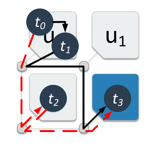
In this work, we concentrate on periodic real-time applications (e.g. image/signal processing, control loops, streaming and multimedia applications, etc.). Such applications typically can be represented by acyclic, directed, bipartite task graphs. Fig. 3(a) illustrates an example. A task graph is denoted by . The vertices are composed of the set of tasks , representing sequential code segment, and the set of messages , representing data exchanged between pairs of tasks. Consequently, tasks in are connected through directed edges in with messages in and vice versa, i.e., .
Applications represented by task graphs shall be executed periodically once admitted with period and have to meet a certain deadline . Furthermore, we assume that the period is at least as long as the deadline. Every message has a maximum data size (i.e., payload), so that together with the period, a minimum bandwidth requirement can be calculated. Each task is assumed to represent a sequentially executed code segments of each application, a WCET (WCET) can be determined through WCET analysis11 1 We assume architectures with tiles consisting of a single PE and analyzable cache, e.g. PowerPC with partitioned LRU cache Wilhelm et al. (2008). for each task on resource . The determination of task WCETs itself is not in the focus of this work but can be derived by WCET analysis tools like aiT Ferdinand (2004) or Chronos Li et al. (2007). However, to prevent cache interferences in private PE caches when mapping different tasks to the same PE, cache partitioning, private scratchpads, or flushing caches after each scheduling interval (c.f. Wilhelm et al. (2008)) may be considered.

3.2 System Architecture
The system architectures targeted by our approach are many-core systems which consist of a set of heterogeneous PEs . The resource type of a PE is specified by the function . A NoC is used as communication infrastructure where routers are connected with each other and to the PEs via links to form a 2-dimensional mesh topology, as exemplified in Fig. 3(b). Each link has a capacity which is proportional to the link width and the frequency . Moreover, we concentrate on packet-based routing, where messages are partitioned into flits which are transmitted one after the other over the infrastructure. Transmission happens from the sending to the receiving PE along a route of consecutive routers. The distance between two PEs and is determined by a hop count function , i.e., the number of routers along the route.
4 Application Mapping and Static Performance Analysis
The worst-case end-to-end latency of an application depends on its mapping onto the available computing and communication resources. Using the proposed model, this is formulated as a mapping of the application graph onto the architecture graph obtained by binding each task and routing each message:
- a)
Binding represents the assignment of each task to a target PE .
- b)
An example mapping of the introduced task graph from Fig. 3(a) is shown in Fig. 3(c).
For a mapping to be feasible, it must be guaranteed that the end-to-end latency for executing an application does not exceed its deadline . The worst-case end-to-end latency of the application depends on the critical path of the mapped task graph. For determining the critical path, we calculate the end-to-end latency for each path of by summing up the worst-case execution latencies of all tasks in the path and the worst-case communication latencies of all messages in the path. The worst-case end-to-end latency of a path for a given binding and routing may then be calculated according to
| (1) |
The worst-case end-to-end latency is then the latency of the path with the highest worst-case end-to-end latency (i.e., the critical path):
| (2) |
Figure 3(c) presents an example where basically includes two paths from the source task to the sink task . One path is , and the other path is . In the given mapping, and are mapped together on one PE so that does not have to be routed over the NoC but can be established by local memory. Note that the resulting delay for doing so has to be already included in the WCET analysis.
When permitting to execute the application on resources that are potentially shared with other applications, they may interfere and affect each other’s timing behavior. For being able to bound this interference, and thus being able to calculate and without knowing whether and how other applications share resources, composability is required. In the following, we describe techniques for composable communication scheduling and composable task scheduling and their respective worst-case analysis as used in this work. Both techniques are based on the idea of reserving periodically available time slots for data transmission and task scheduling, respectively. The interesting aspect is that the worst-case execution and communication latencies obtained here can be composable even during run-time mapping of new tasks into the system if just certain mapping constraints are satisfied. This will be explained in detail in Sect. 6.
4.1 Composable Communication Scheduling
In order to provide the desired composability, the NoC architecture has to fulfill certain criteria and has to show a predictable timing behavior. One NoC architecture which adheres to these requirements is proposed in Heisswolf et al. (2013). This architecture uses wormhole switching and the concept of VCs to ensure a high throughput and low latencies. Further, GS (GS) connections supporting QoS can be set up and physical links are arbitrated in a weighted round robin fashion for transmitting the flits of the different messages routed over it.
A number of time slots (one slot for transmitting one flit) is periodically available for the overall transmission out of which a budget of time slots can be reserved for the transmission of a message . Note that, in contrast to a global synchronous TDMA like presented in Goossens et al. (2005), only the number and not the position of the allocated time slot is fixed. This increases the utilization while still allowing to compute upper bounds for throughput and worst-case latency.
The worst-case communication latency for transmitting message depends on the number of flits , the length of the route , and the number of reserved time slots and can be calculated as follows Heisswolf et al. (2013):
| (3a) | ||||
| (3b) | ||||
In Eq. 3a, denotes the delay for routing one flit in one router with the frequency . Once the routing decision has been made in one router, one flit per clock cycle () can be transmitted.
Figure 4 illustrates the best case and the worst case for communication latencies with examples. The best case corresponds to the case without any interference. The message can utilize the whole scheduling interval and the transmission delay only depends on the message size , the hop distance , and the router delay (see first summand in Eq. (3a)). The second summand in Eq. (3b) gives the maximal delay possible by interference with other messages. This interference can happen in arbitration intervals and depends on the number of hops.


4.2 Composable Task Scheduling
Composability at PE level is achieved by temporally isolating the execution of tasks on it. Therefore, the processing time on a PE is partitioned into service intervals with fixed time duration. Within a service interval, tasks are scheduled exclusively. We consider service intervals of equal length on each PE type 22 2 Generally, the service intervals on different PEs or PE types could be of different lengths. Our approach could still work here, but for keeping notations simple, we make this assumptions.. Transition between the scheduling of two tasks, i.e., task switching, takes place after each service interval . This incurs an OS (OS) scheduling overhead after each interval denoted by . Service intervals are made available to the tasks in the PE’s waiting queue in a round robin fashion. Each task is assigned with a fixed priority that determines the order in which intervals are allocated to tasks by the scheduler.
This scheduling strategy is illustrated in Fig. 5 for two tasks and in the ready queue of a PE. The priority of task is higher than the priority of task , i. e., (the lower the value the higher is the priority). So, task is assigned the first service interval. Allocation then proceeds by means of round robin scheduling. With the above scheduling mechanism, we develop a performance analysis method next to derive the worst-case execution latency of a task.
As initially stated, it is our goal to achieve a high utilization of the given many-core system despite having to isolate applications from each other in order to satisfy real-time constraints. The worst-case execution latency of a task basically consists of two parts: First, the worst-case execution time of the task without interference . The proposed analysis also considers an upper bound on the number of tasks that could share the same PE, denoted by . Therefore, the second part is the worst-case interference from other tasks that could possibly be mapped and scheduled on the same PE. Thus, the total worst-case execution latency () of a task is given by
| (4) |
As each task is executed in service intervals and considered to finish at the end of an interval, the value of is not necessarily equal to the WCET . 33 3 If considering different frequencies the WCET and the service intervals depend on the frequency , i.e., , , and . To simplify the formulae and w.l.o.g. we omit the frequency parameter in the remaining article. Rather, this value is given by
| (5) |
The above expression is obtained from the fact that each task has to complete service intervals to finish its execution. Moreover, each task execution incurs the OS scheduling overhead every time there is a switch into its service interval from the service interval of the previously scheduled task (cf. Fig. 5).


The worst-case interference from other tasks consists of two components: the worst-case interference before and after the first service interval of , which is given by
| (6) |
Recall being the maximum overall number of tasks allowed to be mapped onto a PE, and let be the predecessor of task in the currently analyzed path of the task graph. Then, worst-case interference before the first service interval is formulated as follows:
| (7) |
If task is mapped on the same PE as task , data is exchanged locally and the number of time intervals with length that has to wait is , as exemplified in Fig. 6(a). On the other hand, if is mapped onto another PE, then the maximum interference is due to the service intervals of the possible number of other tasks () on the PE (see Fig. 6(b)). This is because in the worst case, the message from would have to wait until the service intervals of all other tasks finish.
Worst-case interference after the first service interval is given by
| (8) |
where is the maximal total interference from all the remaining possible tasks between two consecutive service intervals of task . The first part of the equation gives the number of service intervals of task between which interference could happen (analogous to Eq. (5)).
5 Design Space Exploration
Due to our composability assumptions and using the performance analysis techniques presented in Section 4.2, a DSE for finding Pareto-optimal mappings is applied to each application individually. Here, multiple mapping candidates are generated per application with verified real-time properties and optimized objectives. The gain of this separation is that the complexity of analyzing a single application is dramatically reduced over the exploration of a complete system with various application mixes.
To efficiently explore various mappings in our DSE, we apply an approach that combines an EA with a Pseudo-Boolean solver Lukasiewycz et al. (2008). The EA constitutes an iterative optimization process: In the exploration phase a set of new applications mappings is generated by applying genetic operators, and in the evaluation phase, this set is evaluated by using analytical models (e.g. for timing the one presented in Section 4). Both phases are iteratively carried out to obtain a set of better and better solutions over time. In each iteration, the best so far explored, non-dominated mappings are updated and stored in an archive and returned once the DSE terminates (see Fig. 7).
Again, to enable the individual exploration of classes of optimal application mappings by means of a formal analysis, the concept of composability is essential. Composability ensures that the addition of a new application in the mix only has a bounded effect on the performance values obtained for each application that was analyzed completely in isolation without considering the execution behavior of any other application as this would fail due complexity reasons.
5.1 Generation of Feasible Application Mappings
We apply the composable scheduling techniques presented in the last section. This means that an application mapping during DSE is generated by (a) determining a binding of each task and (b) determining a routing of each message . We consider deterministic xy-routing for the messages in the NoC. Routing of each message does, therefore, not have to be explored explicitly, as proposed in Graf et al. (2014), as it is implicit by the binding of the message’s sending and receiving tasks. In addition, also a priority has to be assigned to each task for scheduling tasks on the same PE, and has to be generated for the transmission of each message.
In our approach, unique priorities for each task mapped to the same PE are assigned in the exploration phase. In the evaluation phase, it is checked if the assignment is feasible. Through a depth-first search, we identify if a task is a predecessor of another task on the same PE and change the priorities if required.
Also, has to be explored per message . To satisfy the minimal bandwidth requirements of the message, has to be at least . By using a higher , however, the worst-case end-to-end latency may be reduced. Therefore, the exploration interval of is defined as follows:
Only feasible application mappings are returned in the end. More formally, a mapping is feasible if the following conditions hold:
- •
First, the worst-case end-to-end latency has to stay within the deadline:
(9) - •
- •
Finally, no communication link is overutilized. This means that of all messages that are sent over the same route (same source PE and target PE) do not exceed the overall available budget of time slots . Let be the set of messages that are sent over the same route. This constraint is then formulated as follows:
(11) An example of such an infeasible mapping due to overutilization of a link is illustrated in Fig. 8(a).


5.2 Optimization Objectives and Evaluation
Our DSE considers multiple objectives related to non-functional properties. As modern embedded system have strict energy budgets, it is essential to minimize the energy consumption of application mappings. Therefore, we include energy consumption minimization as one objective in the DSE (Objective I). This maximal energy consumption that is going to be minimized may be the sum of the energy consumed by the PEs and energy which is used to route the message over the NoC :
| (12) | ||||
| (13) |
The maximal energy consumed in the PE is the product of the WCET of the task on the mapped PE and the maximal power consumption for the given resource type which is derived by the function . The energy consumed by the communication infrastructure for a message is directly proportional to the number of hops and used links. We derive from the NoC energy model in Hu and Marculescu (2003); Wolkotte et al. (2005):
| (14) | ||||
| (15) |
In Eq. 14, is the energy consumed per bit inside the router, is the energy consumed on a link, and is the size of the message in bits.
Contrary to conventional exploration, the outcome of the DSE will not be used to encode a concrete task and communication assignment to be selected by the RM but rather a class of mappings. More details are elaborated in Section 6. In order to find mappings that allow a greater run-time flexibility, we therefore also include objectives that quantify the resource overhead and flexibility of an application mapping as follows:
The overall number of messages routed over the NoC should be minimized (Objective II). The reason is that, if two communicating tasks are mapped to the same PE, they can exchange their data through local memory and hence . This does not burden the NoC infrastructure. Consequently, congestion on NoC links is reduced, making it more likely to map this operating point at run time.
Another two objectives are the maximization of the average and the minimal hop distances (Objective III and IV). Again, here the idea is to increase flexibility by giving preference to routings that are more likely to be feasibly routed during run time: the longer routes are allowed to be, the less mapping restrictions exist.
As the targeted architecture is heterogeneous, different PE types may be selected for the execution of the tasks. Only minimizing the overall number of allocated PEs without differentiating between their resource types, will result in the generation of suboptimal mappings, e.g., by always using the same PE type such as a powerful core which can execute many tasks within the application’s period. However, if now during run time all instances of this PE type are occupied, no more operating points could be embedded in the system. To thwart this, we minimize the number of allocated PEs per resource type to generate diverse operating points (Objective V).
6 Run-time Constraint Solving
The Pareto-optimal mappings generated by the DSE are handed over to the RM. Yet each DSE mapping corresponds to a fixed assignment of tasks to concrete resources in the architecture. However, in architectures with a multitude of equal resources, numerous equivalent mappings may exist. Therefore, we transform the application mapping (provided by and ) into a constraint graph as exemplified in Fig. 9 right. This graph represents a full class of symmetrical feasible mappings within the NoC which are all equivalent to the application mapping that was actually determined and analyzed during DSE. Consequently, all analyzed properties—particularly real-time properties—also apply for these symmetrical mappings.

6.1 Constraint Graphs
As illustrated in Fig. 9, the vertices of a constraint graph are composed of task clusters belonging to the set and message clusters belonging to the set .
Each task cluster represents a set of tasks that are mapped to the same PE, so that .
Each task cluster is annotated with , specifying the PE type onto which the tasks are mapped, and furthermore, with load induced by the tasks on this PE:
| (16) |
Also, the scheduling information is annotated to the task cluster, i.e., the maximum number of tasks allowed on the PE for scheduling and the priorities of all its tasks.
Each message cluster represents a set of all messages which are routed along the same path in the NoC between two such task clusters, so that . Each message cluster is annotated also with the routing information, i.e. the accumulated and the hop distance between the sending and the receiving task clusters of messages .
6.2 Serializing Operating Points
To hand over the set of operating points to the RM the data has to be serialized. This includes the constraint graph as well as the values for the explored objectives. The memory requirement for these tuples can be calculated as follows:
| (17) |
Where is the memory requirement of the serialized constraint graph, is the number optimized objectives and is the memory requirement of one objective value. For serializing the constraint graph the graph needs to be traversed and all task clusters, all message clusters, and all edges have to be serialized.
| (18) |
For a task cluster, a constraint graph unique ID, the number of tasks , the load , the number of additional tasks , and the priorities of the tasks need to be saved. The serialized message clusters include an ID, the hop constraint , and the SL constraint . With , , , , , , and would result in and .
6.3 Run-time Mapping of Constraint Graphs
The main task of the RM is to select a suitable operating point of the application that should be executed and do the actual run-time application mapping. In principal, the RM can select any operating point out of all found points which fulfills the application’s requirement, e.g. performance.44 4 A methodology to order and select OPs for energy-efficient mappings can be found in Wildermann et al. (2015). To fulfill system requirements, e.g. utilization, the RM may also re-map an already mapped application to another operating point. The step of run-time application mapping itself is to find a concrete application mapping based on the notation of a constraint graph and the architecture by (a) binding each task cluster to a PE, i.e. , and (b) routing each message cluster over a route of consecutive links, i.e., .55 5 Note the difference of the binding and routing to and during DSE. Instead of mapping the task graph onto the architecture, mapping the constraint graph has a lot of advantages: As tasks are clustered to a task cluster and messages to a message cluster, it is evident that and . In consequence, the size of the graph that needs to be mapped during run time is smaller than the original size of the task graph. Second, the constraint graph also is a very compact representation of possibly multiple symmetrical run-time mappings. This basic idea is illustrated in Fig. 10, where one constraint graph can be feasibly mapped in multiple ways while guaranteeing the analyzed quality bounds. Third, time-consuming analysis is performed at design time. The analyzed properties apply for a mapped constraint graph due to the composability of our approach.

A feasible mapping of a constraint graph has to satisfy the following constraints: First, the routings of all message clusters have to fulfill constraints C.1 and C.2:
- C.1
Routing has to provide a connected route of links between and , i.e., the target PEs of its sending and receiving task clusters are and , respectively, with . The hop count of this route must not exceed the given maximal hop count associated with the message cluster:
(19) - C.2
Let denote the set of all already routed message clusters in the system. The accumulated of the messages routed over each link must not exceed the maximal number of time slots :
(20) Figure 8(b) gives an example where this constraint is violated resulting in an infeasible run-time mapping.
Second, the bindings of all task clusters have to fulfill constraints C.3–C.5:
- C.3
The resource type of the target PE has to be the same as is required for the task cluster:
(21) - C.4
Let denote the set of task clusters that are already bound. The load induced by all task clusters which are mapped on a target PE together with the load of the new task cluster must not exceed :
(22) - C.5
| (23) |

In case of a spatial isolation, only constraint C.3 and the absence of other tasks on would be sufficient to guarantee the worst-case latency (see Eq. (4)) as only tasks of one task cluster would be mapped together onto the same PE. However, when applying temporal isolation, all constraints need to hold. Figure 8(c) exemplifies a feasible run-time mapping which fulfills all mentioned constraints. If all constraints are fulfilled but the priority ranges of the tasks in and in overlap, the priorities of are shifted after mapping to keep them unique on the PE. An example of this priority assignment and constraint C.5 can be found in Fig. 11.
6.4 Backtracking Algorithm
To find a mapping which satisfies all the five constraints given a constraint graph and to solve the corresponding CSP66 6 The mapping of the constraint graph is a variant of task mapping which can be modeled as a bin-packing problem which is NP-complete Brião et al. (2008). , we propose a backtracking algorithm as shown in Algo. 1 and is an extension of the algorithm presented in Weichslgartner et al. (2014). This algorithm is executed for each application that should be started on the system. This algorithm starts with and then searches recursively for a valid variable assignment for . As the backtracking algorithm would search exhaustively through all possible variable assignments, a timeout can be chosen to determine the maximal run time of the algorithm. This condition is checked in line 1, and returns an empty set if the maximal time has elapsed since the initial start of the backtracking algorithm for one operating point. In line 1, the next task cluster to map is selected, and in line 1 the domain containing all target PEs which fulfill C.1 and C.3 is created. In lines 1 to 1, the remaining constraints are checked when trying to map to the selected PE . We use xy-routing to obtain routes deterministically for all message clusters sent or received by and which communication partners are already mapped.
7 Experiments
We use task graphs from the Embedded System Synthesis Benchmarks Suite (E3S) Dick (2010) for our experiments. These applications stem from various embedded domains like automotive ( tasks), telecommunication ( tasks), consumer ( tasks), and networking ( tasks). The values for energy consumption, WCET of a task, and bandwidth requirements of messages reflect a realistic scenario of current embedded MPSoCs. We derived the energy consumption of each task on a certain PE from the E3S benchmark and the communication energy consumption by a model proposed by Hu and Marculescu (2003); Wolkotte et al. (2005) with a link length of (resulting in ) and (see Section 5.2).
Furthermore, we selected a heterogeneous NoC-based architecture,consisting of three different processor types from Dick (2010), including an IBM Power PC and variants of AMD K6.
7.1 Considering Communication Constraints
In a first experiment, we evaluate the influence of the communication constraints, i.e. C.1 - C.2, on finding feasible mappings. As exemplified in Fig. 8, checking only the availability of the needed processing resources, e.g. as proposed in Ykman-Couvreur et al. (2006); Shojaei et al. (2013); Wildermann et al. (2014) or assuming only point-to-point connections Singh et al. (2013a), is not sufficient for a feasible mapping in a packet-switched NoC architecture. Indeed, it only satisfies C.3 and neglects the other constraints. To visualize this, we tried, in 6,000 test cases, to map operating points from the above mentioned E3S benchmark applications to a preoccupied system using Algo. 1 without a timeout. As a result, Fig. 12 shows the gap between only considering the resource availability (blue curve) and the actual feasibility considering the communication constraints C.1 and C.2 tested by the introduced constraint solver (red curve). The utilization classes on the x-axis denote the percentage of utilized computing resources before testing to add the new application. For example, 0 represents a completely empty system and the utilization class 10 includes systems where 1 to of the PEs are utilized by previously mapped applications. The gray area between the two curves highlights the optimism introduced by a run-time system which only relies on computing resource availability as in Singh et al. (2013a). In case of a utilization class, of applications could be mapped to the system by only considering resource availability, while only for guarantees for holding their deadlines could be given. All remaining ones miss deadlines because of communication latencies or are actually not mapped because of congested communication resources. Overall, this underlines the importance of considering communication and routing constraints when it comes to methodologies for application mappings on composable NoC-based MPSoCs with a predictable execution times.
7.2 Temporal Isolation versus Spatial Isolation
By applying the EA-based DSE illustrated in Fig. 7, we generated and evaluated an overall of 200,000 mappings per application, resulting from a population size of 200 and 1000 iterations. For each of these mappings, we conducted the performance analysis proposed in Section 4. This was done with the number of additional tasks set to , , and . As outlined in Section 5.2, the optimization criteria were minimizing (I) the energy consumption of each mapping, (II) the number of routed messages, (V) the number of allocated PEs per resource type . Further criteria were maximizing (III) the average and (IV) the minimal hop distance in order to generate more flexible mappings (the bigger the hop count of a message cluster, the less stringent becomes constraint C.1). Out of these 200,000 mappings, all Pareto-optimal solutions which do not violate the application deadline are stored as operating points together with the created constraint graphs and the values of the evaluated objectives (less than 100 points per application).
We then implemented an RM for mapping different run-time mixes of the benchmark applications, where the applications are mapped iteratively. The operating points of each application were sorted in increasing order of energy consumption values (the objective of main interest in our experiments). In this order, a run-time embedder, following a first-fit scheme, searches the first operating point whose constraint graph can be feasibly mapped to the system. For comparison, we implemented two embedder variants based on Algo. 1: (a) variant ti performs the proposed mapping with temporal isolation and (b) variant spi with spatial isolation (see Weichslgartner et al. (2014)).77 7 In both variants, only operating points are used which do not violate the deadline, hence both satisfy the real-time requirements. These embedders try to map one constraint graph of each application (from the first fitting OP) to the architecture. Here, the mapping of the applications is incremental, i.e. first, a constraint graph from the first application is mapped, then a constraint graph from the second application etc. This simulates the arrival of different applications at different points in time during run time that constitute an application mix, which was unknown at design time. In principle, the proposed run-time mapping would also support the remapping of OPs and removing of mapped applications but this is not considered in the following experiments.
We evaluated how many applications out of an application mix we can map successfully to our system (referred as success rate in the following) for both variants. For three different application mixes, experiments were repeatedly performed, but PEs were successively made unavailable for mapping any tasks so that the overall PE availability ranged from down to (which also captures scenarios with, e.g., faulty or powered down PEs). We generated different sequences in which PEs are randomly made unavailable, starting from availability of PEs down to , and used the average values per number of available PEs as the result.
The result of such a set of experiments is depicted in Fig. 13(a) for application mix 1 consisting of one telecom application and two networking applications. Application mix 2 (see Fig. 13(b)) is composed of one telecom, three automotive and one consumer application, while application mix 3 (see Fig. 13(c)) consists of two automotive, two consumer and two networking applications. In the graphs, the x-axis represents the percentage of initially available PEs while the y-axis corresponds to the ratio of successful mappings. The main trend observed is that with decreasing PE availability, the success rate declines much faster when using spatial isolation. In the case of application mix 1, the success rate of spi drops to while it still remains at using the proposed ti in case of an availability of of the PEs. The experiments with application mix 2 show a similar behavior. Even more drastically, in the experiments with application mix 3, all applications could be mapped with our proposed approach in the case where all PEs are available, whereas using spi, one application in the mix could not even be mapped at all.
In our test cases, the obtained energy consumptions of ti mappings were always equal or better than those using spi mappings for a PE availability of for application mixes 1 and 2. In application mix 1, ti and spi reached the same results. In application mix 2, ti mapped operating points with an energy consumption of , whereas spi mapping resulted in per execution. Being able to obtain run-time application mappings which are better with respect to the objective (energy) is a direct consequence of being able to better utilize the available resources. For all other rates of PE availability and also for PE availability in application mix 3, a comparison is not meaningful as spi is not able to map as many applications as ti.
7.3 Execution Time
Constraint solving is the central concept for making use of the offline explored operating points at run time. However, this implies an additional overhead for determining a feasible mapping based on the provided constraint graphs. In this experiment, we evaluate the execution times of the run-time backtracking mapping algorithm (Algo. 1) performed by a central RM. Here, we applied Roloff et al. (2015) to simulate the execution of the RM according to Wildermann et al. (2015) on a embedded processor with a clock frequency of . Overall, feasible mappings for constraint graphs on an NoC architecture were searched via the backtracking mapping algorithm. Figure 14 shows the CDF (CDF) of the execution times (in ) measured for executing the run-time backtracking algorithm. The CDF describes the maximal execution time needed by the percentage of runs. Values are separated for the cases of (a) successful (i.e. at least one feasible mapping exists) and (b) failed constraint solving (no feasible mapping exists). Note that constraint solving is a complex task (in the worst-case, Algo. 1 has exponential run time) and took up to (denoted in the Fig. 14 by a vertical line) for successful and for failed mappings. The vast majority of the applications can be mapped much faster, e.g., of the successful test cases took at most . In the case of failed mappings, execution times were much higher. Only of test cases took below , and took seconds or even minutes (see Fig. 14(b)).
Note that this time only elapses before a newly arriving real-time application is started. While we are dealing with applications that—once mapped—are periodically executed for a long time, mapping times in the range of few seconds might be tolerable. However, in order to bound the execution time of the run-time mapping and supporting domains where mapping time matters, we propose the usage of a timeout mechanism (see Algo. 1): We stop the algorithm after the expiration of the timeout interval and classify the currently tested mapping as infeasible. The timeout value needs to be appropriately chosen to fulfill the turn-around time requirements of the application being mapped. Particularly, as a too low value may increase the number of false negatives (i.e. feasible mappings which are classified as infeasible). However, for our experiments even with a timeout value as low as , we would only reject feasible mappings (i.e., classify false negatives) in of the cases. As we provide multiple operating points per application, a mapping according to another constraint graph may then be obtained.
Nevertheless, to handle larger systems the execution times of this algorithm may be not acceptable anymore. Therefore, we will conduct further research on the run-time CSP (CSP) solving. This may include a hierarchical decomposition of the architecture where the backtracking algorithm searches in a sub-architecture first, distributed CSP solving, or dedicated hardware support Weichslgartner et al. (2015). With using isolated regions per applications, also fast heuristics solving a 2D packing problem can be used Weichslgartner et al. (2016). However, this makes use of spatial isolation only and makes temporal isolation infeasible, thus, decreasing the utilization.
8 Conclusions
In this article, we proposed a technique to increase the utilization of many-core systems using hybrid application mapping combined with a static performance analysis considering bounds on temporal interference on tasks. More specifically, the design-time analysis for applications with real-time constraints was performed considering, for the first time in a hybrid application mapping approach, temporal isolation of concurrent tasks with bounds on task interference. Via DSE (DSE) of mappings, a set of Pareto-optimal operating points with composable performance values is obtained. The subsequent operating point mapping at run time is achieved by solving a constraint satisfaction problem. It has been shown that this hybrid approach allows to provide predictable application mappings within high system utilization and reduced number of PEs that are needed to execute various application mixes while satisfying real-time requirements. Another major advantage of our approach over previous work is the reduction of the exploitative search for feasible mappings to design time and leave only the remaining freedom in finding a concrete mapping to the RM (RM). This was possible through the concept of a constraint graph characterizing feasible mappings. In the future, we want to investigate scalability enhancements of our run-time mapping approach, e.g. distributed constraint solving techniques.
Acknowledgment
This work was supported by the German Research Foundation (DFG) as part of the Transregional Collaborative Research Center “Invasive Computing” (SFB/TR 89).
References
- Akesson et al. (2011) Benny Akesson, Anca Molnos, Andreas Hansson, Jude Ambrose Angelo, and Kees Goossens. 2011. Composability and Predictability for Independent Application Development,Verification, and Execution. In Multiprocessor System-on-Chip, Michael Hübner and Jürgen Becker (Eds.). Springer, New York, NY, USA, 25–56. DOI:http://dx.doi.org/10.1007/978-1-4419-6460-1_2
- Blickle et al. (1998) Tobias Blickle, Jürgen Teich, and Lothar Thiele. 1998. System-Level Synthesis Using Evolutionary Algorithms. Des. Autom. Embedded Syst. 3, 1 (Jan. 1998), 23–58. DOI:http://dx.doi.org/10.1023/A:1008899229802
- Brião et al. (2008) Eduardo Wenzel Brião, Daniel Barcelos, and Flávio Rech Wagner. 2008. Dynamic Task Allocation Strategies in MPSoC for Soft Real-time Applications. In Proceedings of the Conference on Design, Automation and Test in Europe (DATE ’08). ACM, New York, NY, USA, 1386–1389. DOI:http://dx.doi.org/10.1145/1403375.1403709
- Carara et al. (2011) Everton Carara, Gabriel Marchesan Almeida, Gilles Sassatelli, and Fernando Gehm Moraes. 2011. Achieving composability in NoC-based MPSoCs through QoS management at software level. In Proceedings of Design, Automation Test in Europe Conference Exhibition (DATE). 407–412. DOI:http://dx.doi.org/10.1109/DATE.2011.5763071
- Carvalho et al. (2007) Ewerson Carvalho, Ney Calazans, and Fernando Moraes. 2007. Heuristics for Dynamic Task Mapping in NoC-based Heterogeneous MPSoCs. In Proceedings of the 18th IEEE/IFIP International Workshop on Rapid System Prototyping. IEEE, Washington, DC, USA, 34–40. DOI:http://dx.doi.org/10.1109/rsp.2007.26
- Che and Chatha (2010) Weijia Che and Karam S. Chatha. 2010. Scheduling of synchronous data flow models on scratchpad memory based embedded processors. In 2010 International Conference on Computer-Aided Design, ICCAD 2010, San Jose, CA, USA, November 7-11, 2010, Louis Scheffer, Joel R. Phillips, and Alan J. Hu (Eds.). IEEE, 205–212. DOI:http://dx.doi.org/10.1109/ICCAD.2010.5654150
- Choi et al. (2012) Junchul Choi, Hyunok Oh, Sungchan Kim, and Soonhoi Ha. 2012. Executing synchronous dataflow graphs on a SPM-based multicore architecture. In The 49th Annual Design Automation Conference 2012, DAC ’12, San Francisco, CA, USA, June 3-7, 2012, Patrick Groeneveld, Donatella Sciuto, and Soha Hassoun (Eds.). ACM, 664–671. DOI:http://dx.doi.org/10.1145/2228360.2228480
- Chou et al. (2008) Chen-Ling Chou, Umit Y. Ogras, and Radu Marculescu. 2008. Energy- and Performance-Aware Incremental Mapping for Networks on Chip With Multiple Voltage Levels. IEEE Trans. on CAD of Integrated Circuits and Systems 27, 10 (2008), 1866–1879. DOI:http://dx.doi.org/10.1109/TCAD.2008.2003301
- Dally and Towles (2001) William J. Dally and Brian Towles. 2001. Route packets, not wires: on-chip inteconnection networks. In Proceedings of the 38th annual Design Automation Conference (DAC ’01). ACM, New York, NY, USA, 684–689. DOI:http://dx.doi.org/10.1145/378239.379048
- Dick (2010) Robert Dick. 2010. Embedded System Synthesis Benchmarks Suite (E3S). (2010). http://ziyang.ewecs.umich.edu/dickrp/e3s/.
- Ferdinand (2004) Christian Ferdinand. 2004. Worst Case Execution Time Prediction by Static Program Analysis. In 18th International Parallel and Distributed Processing Symposium (IPDPS 2004), 26-30 April 2004, Santa Fe, New Mexico, USA. 125–127. DOI:http://dx.doi.org/10.1109/IPDPS.2004.1303088
- Goossens et al. (2005) Kees Goossens, John Dielissen, and Andrei Radulescu. 2005. Æthereal Network on Chip: Concepts, Architectures, and Implementations. IEEE Design and Test of Computers 22, 5 (2005), 414–421. DOI:http://dx.doi.org/10.1109/MDT.2005.99
- Graf et al. (2014) Sebastian Graf, Felix Reimann, Michael Glaß, and Jürgen Teich. 2014. Towards Scalable Symbolic Routing for Multi-Objective Networked Embedded System Design and Optimization. In Proceedings of the International Conference on Hardware/Software Codesign and System Synthesis (CODES+ISSS 2014). ACM, New York, NY, USA, Article 2, 10 pages. DOI:http://dx.doi.org/10.1145/2656075.2656102
- Heisswolf et al. (2013) Jan Heisswolf, Ralf König, Martin Kupper, and Jürgen Becker. 2013. Providing Multiple Hard Latency and Throughput Guarantees for Packet Switching Networks on Chip. Comput. Electr. Eng. 39, 8 (Nov. 2013), 2603–2622. DOI:http://dx.doi.org/10.1016/j.compeleceng.2013.06.005
- Henkel et al. (2013) Jörg Henkel, Lars Bauer, Nikil Dutt, Puneet Gupta, Sani Nassif, Muhammad Shafique, Mehdi Tahoori, and Norbert Wehn. 2013. Reliable On-chip Systems in the Nano-era: Lessons Learnt and Future Trends. In Proceedings of the 50th Annual Design Automation Conference (DAC ’13). ACM, New York, NY, USA, Article 99, 10 pages. DOI:http://dx.doi.org/10.1145/2463209.2488857
- Hölzenspies et al. (2008) Philip K. F. Hölzenspies, Johann L. Hurink, Jan Kuper, and Gerard J. M. Smit. 2008. Run-time Spatial Mapping of Streaming Applications to a Heterogeneous Multi-processor System-on-chip (MPSoC). In Proceedings of the Conference on Design, Automation and Test in Europe (DATE ’08). ACM, New York, NY, USA, 212–217. DOI:http://dx.doi.org/10.1145/1403375.1403427
- Hu and Marculescu (2003) Jingcao Hu and Radu Marculescu. 2003. Energy-aware Mapping for Tile-based NoC Architectures Under Performance Constraints. In Proceedings of the 2003 Asia and South Pacific Design Automation Conference (ASP-DAC ’03). ACM, New York, NY, USA, 233–239. DOI:http://dx.doi.org/10.1145/1119772.1119818
- Jung et al. (2014) Hanwoong Jung, Chanhee Lee, Shin-Haeng Kang, Sungchan Kim, Hyunok Oh, and Soonhoi Ha. 2014. Dynamic Behavior Specification and Dynamic Mapping for Real-Time Embedded Systems: HOPES Approach. ACM Trans. Embedded Comput. Syst. 13, 4s (2014), 135:1–135:26. DOI:http://dx.doi.org/10.1145/2584658
- Kang et al. (2012) Shin-Haeng Kang, Hoeseok Yang, Lars Schor, Iuliana Bacivarov, Soonhoi Ha, and Lothar Thiele. 2012. Multi-objective mapping optimization via problem decomposition for many-core systems. In IEEE 10th Symposium on Embedded Systems for Real-time Multimedia, ESTIMedia 2012, Tampere, Finland, October 11-12, 2012. IEEE Computer Society, 28–37. DOI:http://dx.doi.org/10.1109/ESTIMedia.2012.6507026
- Kobbe et al. (2011) Sebastian Kobbe, Lars Bauer, Daniel Lohmann, Wolfgang Schröder-Preikschat, and Jörg Henkel. 2011. DistRM: Distributed Resource Management for On-chip Many-core Systems. In Proceedings of the Seventh IEEE/ACM/IFIP International Conference on Hardware/Software Codesign and System Synthesis (CODES+ISSS ’11). ACM, New York, NY, USA, 119–128. DOI:http://dx.doi.org/10.1145/2039370.2039392
- Li et al. (2007) Xianfeng Li, Yun Liang, Tulika Mitra, and Abhik Roychoudhury. 2007. Chronos: A timing analyzer for embedded software. Science of Computer Programming 69, 1 (2007), 56–67.
- Lukasiewycz et al. (2008) Martin Lukasiewycz, Michael Glaß, Christian Haubelt, and Jürgen Teich. 2008. Efficient symbolic multi-objective design space exploration. In Proceedings of the 13th Asia South Pacific Design Automation Conference, ASP-DAC 2008, Seoul, Korea, January 21-24, 2008. IEEE, 691–696. DOI:http://dx.doi.org/10.1109/ASPDAC.2008.4484040
- Mariani et al. (2010) Giovanni Mariani, Prabhat Avasare, Geert Vanmeerbeeck, Chantal Ykman-Couvreur, Gianluca Palermo, Cristina Silvano, and Vittorio Zaccaria. 2010. An industrial design space exploration framework for supporting run-time resource management on multi-core systems. In Design, Automation and Test in Europe, DATE 2010, Dresden, Germany, March 8-12, 2010, Giovanni De Micheli, Bashir M. Al-Hashimi, Wolfgang Müller, and Enrico Macii (Eds.). IEEE Computer Society, 196–201. DOI:http://dx.doi.org/10.1109/DATE.2010.5457211
- Mariani et al. (2012) Giovanni Mariani, Vlad Mihai Sima, Gianluca Palermo, Vittorio Zaccaria, Cristina Silvano, and Koen Bertels. 2012. Using multi-objective design space exploration to enable run-time resource management for reconfigurable architectures. In 2012 Design, Automation & Test in Europe Conference & Exhibition, DATE 2012, Dresden, Germany, March 12-16, 2012, Wolfgang Rosenstiel and Lothar Thiele (Eds.). IEEE, 1379–1384. DOI:http://dx.doi.org/10.1109/DATE.2012.6176578
- Orsila et al. (2007) Heikki Orsila, Tero Kangas, Erno Salminen, Timo D. Hämäläinen, and Marko Hännikäinen. 2007. Automated Memory-aware Application Distribution for Multi-processor System-on-Chips. J. Syst. Archit. 53, 11 (Nov. 2007), 795–815. DOI:http://dx.doi.org/10.1016/j.sysarc.2007.01.013
- Quan and Pimentel (2015) Wei Quan and Andy D. Pimentel. 2015. A Hybrid Task Mapping Algorithm for Heterogeneous MPSoCs. ACM Transactions on Embedded Computing Systems (TECS) 14, 1 (2015), 14:1–14:25. DOI:http://dx.doi.org/10.1145/2680542
- Roloff et al. (2015) Sascha Roloff, David Schafhauser, Frank Hannig, and Jürgen Teich. 2015. Execution-driven Parallel Simulation of PGAS Applications on Heterogeneous Tiled Architectures. In Proceedings of the 52Nd Annual Design Automation Conference (DAC ’15). ACM, New York, NY, USA, Article 44, 6 pages. DOI:http://dx.doi.org/10.1145/2744769.2744840
- Shojaei et al. (2013) Hamid Shojaei, Twan Basten, Marc Geilen, and Azadeh Davoodi. 2013. A Fast and Scalable Multidimensional Multiple-choice Knapsack Heuristic. TODAES 18, 4, Article 51 (2013), 32 pages.
- Shojaei et al. (2009) H. Shojaei, A. Ghamarian, T. Basten, M. Geilen, S. Stuijk, and R. Hoes. 2009. A parameterized compositional multi-dimensional multiple-choice knapsack heuristic for CMP run-time management. In 2009 46th ACM/IEEE Design Automation Conference. 917–922. DOI:http://dx.doi.org/10.1145/1629911.1630147
- Singh et al. (2013a) Amit Kumar Singh, Akash Kumar, and Thambipillai Srikanthan. 2013a. Accelerating Throughput-aware Runtime Mapping for Heterogeneous MPSoCs. ACM Trans. Des. Autom. Electron. Syst. 18, 1, Article 9 (Jan. 2013), 29 pages. DOI:http://dx.doi.org/10.1145/2390191.2390200
- Singh et al. (2013b) Amit Kumar Singh, Muhammad Shafique, Akash Kumar, and Jörg Henkel. 2013b. Mapping on Multi/Many-core Systems: Survey of Current and Emerging Trends. In Proceedings of the 50th Annual Design Automation Conference (DAC ’13). ACM, New York, NY, USA, Article 1, 10 pages. DOI:http://dx.doi.org/10.1145/2463209.2488734
- van Stralen and Pimentel (2010) Peter van Stralen and Andy D. Pimentel. 2010. Scenario-based design space exploration of MPSoCs. In Proceedings of Conference on Computer Design (ICCD). 305–312.
- Weichslgartner et al. (2014) Andreas Weichslgartner, Deepak Gangadharan, Stefan Wildermann, Michael Glaß, and Jürgen Teich. 2014. DAARM: Design-time Application Analysis and Run-time Mapping for Predictable Execution in Many-core Systems. In Proceedings of the 2014 International Conference on Hardware/Software Codesign and System Synthesis (CODES ’14). ACM, New York, NY, USA, Article 34, 10 pages. DOI:http://dx.doi.org/10.1145/2656075.2656083
- Weichslgartner et al. (2015) Andreas Weichslgartner, Jan Heisswolf, Aurang Zaib, Thomas Wild, Andreas Herkersdorf, Jürgen Becker, and Jürgen Teich. 2015. Position Paper: Towards Hardware-Assisted Decentralized Mapping of Applications for Heterogeneous NoC Architectures. In Proceedings of the second International Workshop on Multi-Objective Many-Core Design (MOMAC) in conjunction with International Conference on Architecture of Computing Systems (ARCS). IEEE, 1–4.
- Weichslgartner et al. (2016) Andreas Weichslgartner, Stefan Wildermann, Johannes Götzfried, Felix C. Freiling, Michael Glaß, and Jürgen Teich. 2016. Design-Time/Run-Time Mapping of Security-Critical Applications in Heterogeneous MPSoCs. In Proceedings of the 19th International Workshop on Software and Compilers for Embedded Systems, SCOPES 2016, Sankt Goar, Germany, May 23-25, 2016, Sander Stuijk (Ed.). ACM, 153–162. DOI:http://dx.doi.org/10.1145/2906363.2906370
- Weichslgartner et al. (2011) Andreas Weichslgartner, Stefan Wildermann, and Jürgen Teich. 2011. Dynamic Decentralized Mapping of Tree-structured Applications on NoC Architectures. In Proceedings of the Fifth ACM/IEEE International Symposium on Networks-on-Chip (NOCS ’11). ACM, New York, NY, USA, 201–208. DOI:http://dx.doi.org/10.1145/1999946.1999979
- Wildermann et al. (2014) Stefan Wildermann, Michael Glaß, and Jürgen Teich. 2014. Multi-objective distributed run-time resource management for many-cores. In Design, Automation & Test in Europe Conference & Exhibition, DATE 2014, Dresden, Germany, March 24-28, 2014. IEEE, 1–6. DOI:http://dx.doi.org/10.7873/DATE.2014.234
- Wildermann et al. (2011) Stefan Wildermann, Felix Reimann, Daniel Ziener, and Jürgen Teich. 2011. Symbolic Design Space Exploration for Multi-mode Reconfigurable Systems. In Proceedings of the Seventh IEEE/ACM/IFIP International Conference on Hardware/Software Codesign and System Synthesis (CODES+ISSS ’11). ACM, New York, NY, USA, 129–138. DOI:http://dx.doi.org/10.1145/2039370.2039393
- Wildermann et al. (2015) Stefan Wildermann, Andreas Weichslgartner, and Jürgen Teich. 2015. Design Methodology and Run-Time Management for Predictable Many-Core Systems. In Proceedings of the 2015 IEEE International Symposium on Object/Component/Service-Oriented Real-Time Distributed Computing Workshops, ISORC Workshops 2015, Auckland, New Zealand, April 13-17, 2015. IEEE Computer Society, 103–110. DOI:http://dx.doi.org/10.1109/ISORCW.2015.48
- Wilhelm et al. (2008) Reinhard Wilhelm, Jakob Engblom, Andreas Ermedahl, Niklas Holsti, Stephan Thesing, David Whalley, Guillem Bernat, Christian Ferdinand, Reinhold Heckmann, Tulika Mitra, Frank Mueller, Isabelle Puaut, Peter Puschner, Jan Staschulat, and Per Stenström. 2008. The Worst-case Execution-time Problem—Overview of Methods and Survey of Tools. ACM Transactions on Embedded Computing Systems (TECS) 7, 3, Article 36 (May 2008), 53 pages. DOI:http://dx.doi.org/10.1145/1347375.1347389
- Wolkotte et al. (2005) Pascal T Wolkotte, Gerard JM Smit, Nikolay Kavaldjiev, Jens E Becker, and Jürgen Becker. 2005. Energy Model of Networks-on-Chip and a Bus. In System-on-Chip, 2005. Proceedings. 2005 International Symposium on. 82–85. DOI:http://dx.doi.org/10.1109/ISSOC.2005.1595650
- Ykman-Couvreur et al. (2011) Chantal Ykman-Couvreur, Prabhat Avasare, Giovanni Mariani, Gianluca Palermo, Cristina Silvano, and Vittorio Zaccaria. 2011. Linking run-time resource management of embedded multi-core platforms with automated design-time exploration. IET Computers & Digital Techniques 5, 2 (2011), 123–135. DOI:http://dx.doi.org/10.1049/iet-cdt.2010.0030
- Ykman-Couvreur et al. (2006) Chantal Ykman-Couvreur, Vincent Nollet, Francky Catthoor, and Henk Corporaal. 2006. Fast Multi-Dimension Multi-Choice Knapsack Heuristic for MP-SoC Run-Time Management. In System-on-Chip, 2006. International Symposium on. 1–4. DOI:http://dx.doi.org/10.1109/ISSOC.2006.321966