To fix the notation, we shortly outline the construction of tensor product B-splines in the case of $d=2$ dimensions. First we specify the polynomial degrees $(p,q)$ and the horizontal and vertical knot vectors

which contain non-decreasing parametric real values so that

are the multiplicities of the parameter values in the knot vectors (the multiplicity $\mu(X,x)$ is zero if the given value $x$ is not a knot in $X$). We write $M_{i,p}(\xi)$ and $N_{j,q}(\eta)$ for the univariate B-splines, which are computed by means of the recursion [5]

for $j=1,\ldots,n$. Fractions with zero denominators are considered zero. The same recursion applies to $M_{i,p}(\xi)$, replacing $j,q$ in (2.1)–(5) by $i,p$ for $i=1,\ldots,m$.

A function $\mathbf{f}(\xi,\eta):[\xi_{p+1},\xi_{m+1}]\times[\eta_{q+1},\eta_{n+1}]\rightarrow\mathbb{R}^{2}$ is called a bivariate tensor product B-spline function if it has the form

with the de Boor control points $\mathbf{d}_{i,j}\in\mathbb{R}^{2}$, which form the control net associated to the parametric representation. In order to work with the unit square as parameter domain, combined with open knot vectors, we assume additionally $\xi_{1}=\ldots=\xi_{p+1}=0$ and $\xi_{m+1}=\ldots=\xi_{m+p+1}=1$ at the beginning and at the end; analogously $\eta_{1}=\ldots=\eta_{q+1}=0$ and $\eta_{n+1}=\eta_{n+2}=\ldots=\eta_{n+q+1}=1$.

In $d=3$ dimensions, a trivariate B-spline tensor product function is generated analogously, which results in

with an additional set of univariate B-splines $L_{k,r}$ and control points $\mathbf{d}_{i,j,k}\in\mathbb{R}^{3}$.

For the straightforward extension to NURBS, we refer to [16].

In $d=2$ dimensions, an SB-parametrization can be constructed as follows. We assume a star-shaped domain whose boundary is described by a spline curve $\gamma$,

with univariate B-splines $N_{j,q}$ of a certain degree $q$ and control points $\mathbf{c}_{j}\in\mathbb{R}^{2}$. We require $\eta\in[0,1]$ for the independent variable and consider a closed curve with ${\mbox{\boldmath$\gamma$}}(0)={\mbox{\boldmath$\gamma$}}(1)$. This can be achieved by an open knot vector, as described in the previous subsection, and control points $\mathbf{c}_{1}=\mathbf{c}_{n}$. Other situations with several curve segments or wedge-shape geometries will be discussed below.

Next, we pick a point $\mathbf{x}_{0}\in\Omega$, the scaling center, and connect it with the boundary by means of rays that emanate from it, Fig. 2. A ray that reaches from the scaling center to a control point $\mathbf{c}_{j}$ on the boundary can be parametrized as

Replacing the control point $\mathbf{c}_{j}$ by any point on the curve (8), we obtain by the partition of unity

with control points $\mathbf{d}_{1j}:=\mathbf{x}_{0},\,\mathbf{d}_{2j}:=\mathbf{c}_{j},\,j=1,\ldots,n;$ and linear B-splines $M_{1,1}(\xi)=1-\xi,\,\,M_{2,1}(\xi)=\xi$.

The bivariate parametrization $\mathbf{F}(\xi,\eta)$ maps the unit square $\Omega_{0}=[0,1]^{2}$ to the domain $\Omega$ with a multiple control point $\mathbf{d}_{1j}=\mathbf{x}_{0}$ in the scaling center and the other control points $\mathbf{d}_{2j}=\mathbf{c}_{j}$ adopted from the boundary curve. In other words, the left vertical edge of the unit square collapses to the scaling center while the right vertical edge is mapped to the boundary, Fig. 2. Note that the geometry function $\mathbf{F}$ in (10) features the usual tensor product structure (6) with only $m=2$ linear B-splines in $\xi$-direction and $n$ B-splines inherited from the boundary curve in $\eta$-direction.

In some cases it will be advantageous to replace the double sum in (10) by the compact form

which is the usual notation in the SB-FEM [19, 20] and SB-IGA[2, 3, 14]. Here, the matrix $\mathbf{C}:=(\mathbf{c}_{1},\ldots,\mathbf{c}_{n})\in\mathbb{R}^{2\times n}$ contains the control points on the boundary and the vector $\mathbf{N}(\eta):=(N_{1,q}(\eta),\ldots,N_{n,q}(\eta))^{T}\in\mathbb{R}^{n}$ the B-splines.

Finally, we extend the bivariate spline parametrization (10) and apply both knot insertion and degree elevation in radial direction, which preserves the rays that emanate from the scaling center but leads to a more general formulation

Note that the multiple control point in the scaling center is still present here, i.e., $\tilde{\mathbf{d}}_{1j}=\mathbf{x}_{0}$ for $j=1,\ldots,n$ and that $\tilde{\mathbf{d}}_{mj}=\mathbf{c}_{j}$ for the control points of the boundary curve, $j=1,\ldots,n$. The other extra control points $\tilde{\mathbf{d}}_{ij}$ result from the usual steps of knot insertion and degree elevation. In this way, we obtain a finer parametrization that still preserves the scaled boundary idea. At the same time, it possesses a discretization in both $\xi$ and $\eta$ that can be used as natural isogeometric mesh for a numerical simulation.

We aim now at studying the regularity and smoothness of the SB-parametrization. For this purpose, it is convenient to use the representation (11), whose Jacobian reads

Here, we used the notation $\mathbf{c}_{1}^{T}:=\mathbf{C}(1,:)$ for the first and $\mathbf{c}_{2}^{T}:=\mathbf{C}(2,:)$ for the second row of $\mathbf{C}$, respectively. Furthermore, $\mathbf{x}_{0}^{T}=(x_{0,1},x_{0,2})$ and the derivative with respect to $\eta$ is written as $\mathbf{N}^{\prime}=\partial\mathbf{N}/\partial\eta$.

The determinant of the Jacobian is given by

where

The multiplicative structure of the Jacobian allows a straightforward analysis of the parametrization in terms of regularity and smoothness. Obviously, in the scaling center $\mathbf{x}_{0}$ where $\xi=0$ the parametrization $\mathbf{F}$ becomes singular. For the derivative in $\eta$-direction, we have additionally $\partial\mathbf{F}(\xi=0,\eta)/\partial\eta=\mathbf{0}$. The smoothness of the boundary curve $\gamma$, on the other hand, determines the smoothness of $\mathbf{F}$: if $\gamma$ is of class $C^{k}$, then $\mathbf{F}$ is of class $C^{k}$ as well. If $\gamma$ possesses points of reduced smoothness, e.g. an interpolatory knot where the control point $\mathbf{c}_{j}$ lies on the curve, then the ray $(1-\xi)\mathbf{x}_{0}+\xi\mathbf{c}_{j},\,\xi\in[0,1]$, which runs from the scaling center to $\mathbf{c}_{j}$, will inherit the smoothness and form a $C^{0}$-edge in the interior. This reasoning applies also to the regularity. If $\gamma$ is injective, the parametrization will also be injective except for the scaling center.

In passing we note that recently so-called multi-degree polar splines have been introduced as a general alternative to circumvent the singularity in the scaling center [23].

We now turn to extensions of SB-parametrizations.

Several Curve Segments. There are situations where several curve segments are connected in order to define the computational domain $\Omega$. In this case, one can decompose the domain into several wedge-shape objects where each wedge forms a triangle as sketched in Fig. 3 on the left. The scaling center of such a wedge is in one of the vertices, and the two edges that emanate from it are the rays that point to the end points of the curve $\gamma$. The representations (11) and (12) hold also for the parametrization of the wedge. If we combine several curves as in Fig. 3 on the right, we first pick a common scaling center $\mathbf{x}_{0}$, and each wedge possesses then its own parametrization. Due to the connectivity of the boundary curve, however, it is guaranteed that the individual wedges do not intersect and that the domain $\Omega$ is completely covered.

One might wonder whether the situation of several curve segments is actually of relevance since it is always possible to define a new boundary curve that comprises the individual segments. E.g., in Fig. 3 we can set $\tilde{{\mbox{\boldmath$\gamma$}}}:={\mbox{\boldmath$\gamma$}}_{1}\cup{\mbox{\boldmath$\gamma$}}_{2}\cup{\mbox{\boldmath$\gamma$}}_{3}$. The new curve $\tilde{{\mbox{\boldmath$\gamma$}}}$ then might feature interpolatory knots with reduced continuity, but this would mean no obstacle to use it as starting point for a single SB-parametrization (12). Nevertheless, several curve segments are useful as they present a natural decomposition of the domain, similar to a multi-block or multi-patch strcuture, that is inherited from the boundary geometry. Morever, this description provides insight into the 3D case where each curve segment turns into a surface patch with an individual parametrization.

Extensions beyond Star-shaped Domains. Obviously, the restriction to a star-shaped domain is a limitation of SB-parametrizations. We shortly discuss two ways to overcome this drawback.

Consider again the general parametrization (12) where the control points in the interior are given by $\tilde{\mathbf{d}}_{ij}$ for $i=2,\ldots,m-1$ and $j=1,\ldots,n$. If we fix an index $j$ and consider the corresponding ray from the scaling center to the control point $\mathbf{c}_{j}$ on the boundary, it is possible to move the control points $\tilde{\mathbf{d}}_{2,j},\ldots,\tilde{\mathbf{d}}_{m-1,j}$ along the ray such that we obtain a curved ray. This technique can be used to relax the requirement of a star-shaped domain , see Fig. 4 for an example with a rotor geometry that is part of a screw compressor unit. In this figure, the visible mesh on the right consists of the isoparametric lines $\xi=\xi_{k}$ and $\eta=\eta_{\ell}$, which must be distinguished from the control net on the left.

A more general approach relies on methods for the so-called art gallery problem. Basically, this means that for a general domain $\Omega$ such as in Fig. 5, we search for a decomposition into blocks or patches that are star-shaped. If the domain $\Omega$ has a polygonal boundary with $k$ vertices, there is an upper bound on the number of blocks that are required for such a decomposition. The bound is $\lfloor k/3\rfloor$, and there are algorithms that compute the decomposition automatically [15].

Extension to NURBS. If the curve $\gamma$ in (8) is given as linear combination of NURBS [16]

with weights $w_{j},\,j=1,\ldots,n$, the above construction of the SB-parametrization stays the same. Moreover, all the properties discussed so far, including the multiplicative structure of the Jacobian, are preserved.

Extension to THB. It is possible to use local refinement along the boundary, where higher numerical accuracy is often necessary. Fig. 6 shows an example of local refinement using THB-splines [7, 25].

Extension to 3D Geometries. Obviously, the basic idea for constructing an SB-parametrization also carries over to 3D objects that are given in terms of a surface description. For a detailed discussion of this case we refer to [3] where such parametrizations are constructed and combined with SB-IGA. We shortly consider a star-shaped solid $\Omega$ with surface $\partial\Omega$ that is parametrized via

with bivariate B-splines $N_{j,q}L_{k,r}$ and control points $\mathbf{c}_{jk}\in\mathbb{R}^{3}$. In general, there will be several surface patches that are glued together to form the complete surface, but we skip this technical detail. Picking a scaling center $\mathbf{x}_{0}\in\Omega$, we can proceed as in the planar case and write a ray from the center to the surface as

with control points $\mathbf{d}_{1jk}:=\mathbf{x}_{0},\,\mathbf{d}_{2jk}:=\mathbf{c}_{jk},\,j=1,\ldots,n;\,k=1,\ldots,\ell$.

For some geometries, one can also apply the scaled boundary idea only in a cross-section and then extrude the geometry in the third direction, generalizing the concept of cylindrical coordinates.

Next assume that we have a parametrization of $\Omega$ available as in (1). For the differentiation, the chain rule applied to $u(\mathbf{x})=u(\mathbf{F}({\mbox{\boldmath$\xi$}}))=:\hat{u}({\mbox{\boldmath$\xi$}})$ yields, using a row vector notation for the gradient $\nabla u$,

The integrals in the weak form (23) then satisfy the transformation rules

and

The integrals over $\Omega_{0}$ that are defined by the right hand sides of (25) and (26) are at the core of Galerkin-based IGA.

For our purposes, it is now advantageous to adopt a more general viewpoint from differential geometry where the Laplace operator is extended to operate on functions defined on surfaces in Euclidean space and on Riemannian manifolds, see Berger [1]. We define the metric tensor or first fundamental form

which has the determinant $\mbox{det }\mathbf{g}=(\mbox{det }\mathbf{DF})^{2}$. The transformed weak form from (25) and (26) then reads

for test functions $\hat{v}=v\circ\mathbf{F}$. In terms of regularity and smoothness, the parametrization $\mathbf{F}$ is here required to be of class $C^{1}$ and to be injective almost everywhere, which means that singularities in sets of measure zero, such as points, are admitted.

Corresponding to the weak form (28), there is a strong form that makes use of the Laplace–Beltrami operator. Like the standard Laplacian, this operator is defined as the divergence of the gradient in parametric coordinates, and it reads

For the strong form of Poisson’s equation with respect to the metric $\mathbf{g}$ and expressed in the coordinates $\xi$, this implies the representation

Clearly, this requires now the parametrization $\mathbf{F}$ to be of class $C^{2}$ and injective in order to hold in all of $\Omega_{0}$.

The Galerkin projection of the weak form (23) in physical coordinates $\mathbf{x}$ replaces the infinite dimensional space $V$ by a finite dimensional subspace $V_{h}\subset V$, with the subscript $h$ indicating the relation to a spatial grid. Let $\phi_{1},\ldots,\phi_{K}$ be a basis of $V_{h}$, then the numerical approximation $u_{h}$ is constructed as linear combination

with unknown real coefficients $q_{i}\in\mathbb{R}$.

Upon inserting $u_{h}$ into the weak form (23) and testing with $v=\phi_{j}$ for $j=1,\ldots,K$, one obtains the linear system

with $K\times K$ stiffness matrix $\mathbf{A}=(a(\phi_{i},\phi_{j}))_{i,j=1,\ldots,K}$ and right hand side vector $\mathbf{r}=(\langle l,\phi_{i}\rangle)_{i=1,\ldots,K}$. Since the matrix $\mathbf{A}$ inherits the properties of the bilinear form $a$, it is straightforward to show that $\mathbf{A}$ is symmetric positive definite, and thus the numerical solution $\mathbf{q}$ or $u_{h}$, respectively, is well-defined.

In Galerkin-based IGA, we define $\phi_{i}=\psi_{i}\circ\mathbf{F}^{-1},\,i=1,\ldots,K,$ as basis functions via the push forward operator, where $\psi_{i}=M_{j,p}N_{k,q}$ is given by bivariate B-splines in the planar case and $\psi_{i}=M_{j,p}N_{k,q}L_{w,r}$ by trivariate B-splines in the spatial case. The total number of degrees of freedom is accordingly $K=mn$ or $K=mn\ell$, respectively, and the numerical approximation becomes, expressed in parametric coordinates, a bivariate B-spline tensor product function (6) or a trivariate function (7). Overall, this projection step then boils down to inserting $\hat{u}=\sum q_{i}\psi_{i}$ and $\hat{v}=\psi_{j},j=1,\ldots,K,$ into the weak form (28).

In the SB-IGA, we transform first the PDE into the strong form (30) in parametric coordinates, which leads to

Then, a Galerkin projection with respect to the circumferential coordinate $\eta$ is derived, using the given representation of the boundary in terms of the B-splines $\mathbf{N}(\eta)$. We set $\hat{u}(\xi,\eta)=\mathbf{N}^{T}(\eta)\mathbf{U}(\xi),\;\hat{v}(\xi,\eta)=\mathbf{N}^{T}(\eta)\mathbf{V},$ where $\mathbf{U}(\xi)\in\mathbb{R}^{n}$ is the solution depending on the radial parameter $\xi$ and the variations $\mathbf{V}\in\mathbb{R}^{n}$ are arbitrary. We insert $\hat{u}$ in (37), multiply by $\hat{v}$ and integrate with respect to $\eta$. This yields

The fourth integral of equation (38) is integrated by parts, using the property $V_{1}=V_{n}$ that holds for the variations of a periodic curve. Thus it holds

Since (38) must hold for all variations $\mathbf{V}$, we can now perform the integration with respect to $\eta$ and generate a strong form for the vector $\mathbf{U}(\xi)$. For this purpose, we introduce a notation that is common in the SB-FEM and SB-IGA. Define

then (38) becomes

where

We obtain in this way an ODE in the scaling direction $\xi$, with boundary condition $\mathbf{U}(\xi=1)=\mathbf{0}$ and periodicity condition $U_{1}(\xi)=U_{n}(\xi)$.

There are several options for the numerical treatment of the ODE (39) in scaling direction, as proposed in [2, 3, 14]. Besides an analytical approach that is based on the solution of an eigenvalue problem with a Hamiltonian matrix, see Section 4 below, there is also the possibility of using collocation or standard Galerkin projection with respect to the $\xi$-variable. The latter is based on a weak form in $\xi$ which possesses the same structure and the same separation property as shown in (36). For more details, we refer to the above references.

To better understand the singularity at $\xi=0$, we make use of the boundary value problem that is generated by the SB-IGA. In its original form, the SB-FEM, which provides the basic idea for SB-IGA, is a semi-analytical method where the boundary value problem with respect to $\xi$ is solved exactly [18]. We adopt here this approach since it offers insight into the nature of the singularity. For a more general treatment of singularities in IGA see [21, 22].

We consider (39) as homogeneous system (writing $\mathbf{U}_{\xi}=\mathbf{U}^{\prime}$)

with a symmetric positive definite matrix $\mathbf{M}\in\mathbb{R}^{n\times n}$, a symmetric positive semi-definite matrix $\mathbf{K}\in\mathbb{R}^{n\times n}$, and a matrix $\mathbf{C}\in\mathbb{R}^{n\times n}$. Next, we introduce the new variables

The second order ODE is thus transformed to a first order system

with the Hamiltonian matrix

In other words, $\mathbf{H}\in\mathbb{R}^{2n\times 2n}$ becomes a symmetric matrix when multiplied by the skew-symmetric matrix $\mathbf{J}$,

The characteristic polynomial $d(\lambda)=\mbox{det}(\lambda\mathbf{I}_{2n}-\mathbf{H})$ is an even function, which means that the eigenvalues of $\mathbf{H}$ come in pairs $(-\lambda_{i},\lambda_{i})$ with $\mbox{Re}\lambda_{i}\geq 0$. Hence the solution of (42) in the homogeneous case is a linear combination of terms $c_{i}\xi^{\lambda_{i}}{\mbox{\boldmath$\phi$}}_{i}+\hat{c}_{i}\xi^{-\lambda_{i}}\hat{{\mbox{\boldmath$\phi$}}_{i}}$ with corresponding eigenvectors ${\mbox{\boldmath$\phi$}}_{i},\hat{{\mbox{\boldmath$\phi$}}}_{i}$. Since the solution is finite in $\xi=0$, one concludes that $\hat{c}_{i}=0$, which cancels the instable part.

In practice, the numerical solution of the eigenvalue problem for $\mathbf{H}$ is only feasible for comparably small dimensions. But our interest here lies on the insight that we obtain from it. The singularity in the scaling center thus looses its threat. However, the question remains what happens if we apply a discretization with respect to $\xi$ and do not utilize the eigenvalue solution.

We concentrate next on Galerkin-based IGA and discuss the practical treatment of the singularity in the scaling center. In all numerical experiments that we performed so far, the singularity did not really influence the results, and we did not observe an instability nor a singular stiffness matrix. Can we explain this?

Consider the bilinear form (35) in parametric coordinates. The fourth term in the integral is the critical one and it contains the factor $1/\xi$. Analogously to the separation in (36), this term can also be written as the product of a well-defined integral with respect to $\eta$ times the integral

We apply linear B-splines and analyze the contribution of the first element from $0$ to $h$ where $h$ is the mesh size. The integral (43) then yields for $M_{j}=M_{\ell}=M_{1}$

Obviously, the integral over $1/\xi$ diverges while the other terms are not critical. In a numerical implementation, however, quadrature is used instead of exact integration. If we apply the midpoint rule as simple example, we get

The evaluation is thus independent of $h$, and the contribution of this integral to the stiffness matrix is always well-defined.

The above reasoning applies also to B-splines of higher degrees and to higher order quadrature rules as long as the nodes of the quadrature rule are in the interior of $[0,h]$. In this way, we can conclude that the computation of the stiffness matrix in Galerkin-based IGA is not affected by the singularity, cf. [21]. However, at the moment we cannot say whether the convergence of the method is impaired or whether the condition number might become problematic.

Another problem is the smoothness of the numerical solution in the scaling center. The geometry mapping (11) projects the entire side of the parametric domain into the scaling center. Therefore several degrees of freedom correspond to the value there. By construction the solution is continuous around the singularity, however, only neighboring degrees of freedom are related to each other. As a consequence, their values across the singularity do not have to be the same, which results in the discontinuous numerical solution, see Fig. 7.

The continuity of the solution can be restored by imposing an equality constraint on all the degrees of freedom in the scaling center. However, this leads to a saddle point problem if Lagrange multipliers are used. It is also worth mentioning that the significant difference between the initially discontinuous and the constrained continuous solutions is only noticeable for very coarse meshes, while for the number of degrees of freedom large enough the solutions are nearly identical, see Fig. 9 in Section 5.

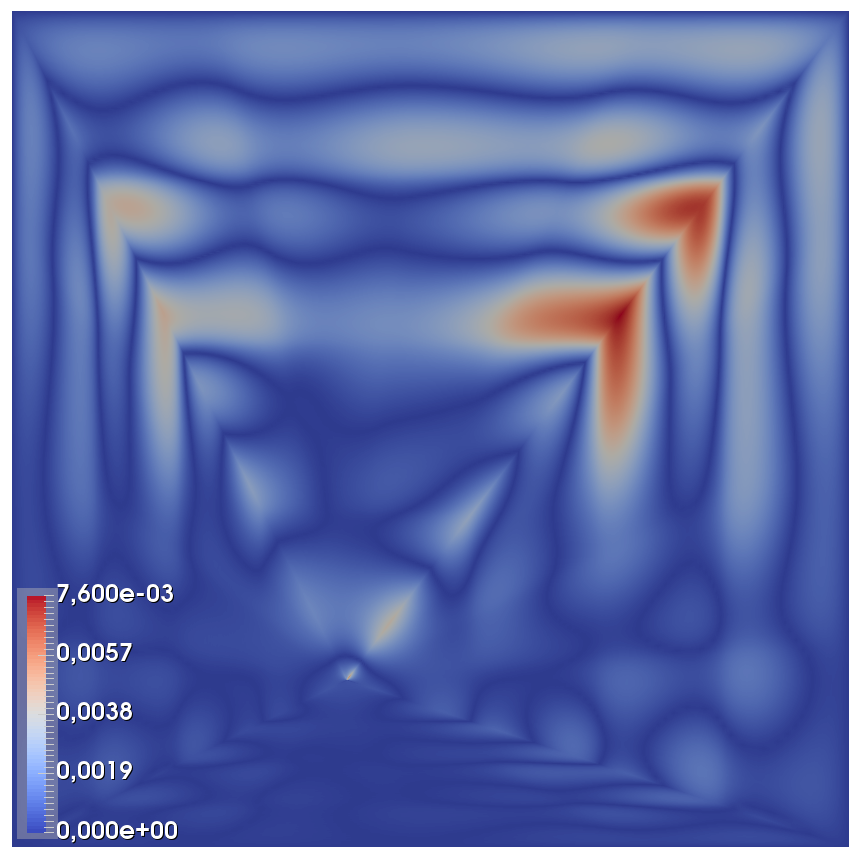
We solve the Poisson problem on a unit square. The simplicity of this geometry allows a large variety of parametrizations to be generated. We select the following for comparison, see Fig. 8: the center scaled as the most natural; the off-center scaled to investigate the influence of the scaling center location on the numerical error; the internally smooth to demonstrate that it is possible to generate an SB-parametrization that does not inherit non-smooth features from the boundary; and the standard rectangular to serve as a reference for comparison. Quadratic splines are used to represent the geometry and to discretize the equation for all parametrizations. We refer to Appendix A for the corresponding knot vectors and control points.

We consider the function

and we impose homogeneous boundary conditions $u=0$ on $\partial\Omega$. The function $u^{*}$ obviously fulfills the boundary conditions, thus it is the unique solution to (18) with $f=-\Delta u^{*}$. We solve (18) using different parametrizations and the known analytical solution is used to compute the numerical error, which is depicted in Fig. 8.

After analyzing the error distribution it is immediately clear that the rectangular parametrization yields the best results. However, it should be noted for the SB-parametrizations that despite the singularity in the scaling center the numerical error is not observably higher there than in the other regions. The center and off-center scaled parametrizations indicate large error concentrations along the $C^{0}$ rays from the corners, whereas for the internally smooth parametrization the error is more distributed and is slightly lower.

We further compare the numerical error for different parametrizations by considering the global $L_{2}$ error while refining the analysis. The results are presented in Fig. 9. The convergence rate for all parametrizations is approximately of order three. The smallest error among the SB-parametrizations is found for the simplest and the most natural center scaled parametrization. Additionally, we do the convergence analysis for the off-center parametrization to study the influence of the singularity treatment as discussed in Subsection 4.2. The difference between the initially discontinuous and the constrained continuous solutions is only observed for a very coarse mesh, whereas for a sufficient number of degrees of freedom the two solutions are virtually identical.

A screw compressor rotor with its intricate non-star-shaped geometry serves as an exemplary industrial application of SB-parametrizations due to a large variety of rotatory mechanisms in engineering.

Here we consider the Poisson problem (18) posed over the rotor geometry. We use the function

with the parameter $a\in\mathbb{R}$ as the Dirichlet boundary condition on $\partial\Omega$, which is enforced strongly. Then $u^{*}$ is the unique solution to (18) with $f=-\Delta u^{*}$. The known analytical solution immediately allows to compute the numerical error, which can be used to measure the quality of the parametrization. The standard rectangular parametrization, which is relatively straightforward to generate in this case due to the presence of four sharp corners, serves as a reference for comparison, see Fig. 10.

Probably the most remarkable result of this comparison is that the singularity in the scaling center does not give rise to any particularly relevant numerical error. Moreover, we note that both parametrizations yield errors of the same order of magnitude. To further study the numerical error, we use its $L_{2}$-norm as a global error and we compare the two parametrizations while refining the analysis. Fig. 11 depicts the results. Both parametrizations demonstrate the convergence rate of roughly third order, and while the rectangular parametrizations offers slightly more accuracy per degree of freedom, the SB-parametrization exhibits a marginally higher convergence rate.

We are grateful to Daniela Fußeder, Carlo Lovadina and Angelos Mantzaflaris for fruitful discussions on the topic of scaled boundary parametrizations and for hints on related fields. Andreas Brümmer and Matthias Utri supplied us with the point cloud data for the rotor example in Fig. 4. Moreover, we acknowledge the support by the European Union under grant no. 678727 (Alexander Shamanskiy, Project MOTOR) and by the German Research Council (DFG) under grant no. SI 756/5-1 (Clarissa Arioli, Project YASON).

Here we describe the simplest and the most natural SB-parametrization of a unit square, which is shown in Fig. 8. The basis is quadratic in both direction, with the knots vectors given by

and

and the control points from Table 1. The resulting planar parametrization inherits $C^{0}$ rays from the four corners of the square, remaining $C^{1}$ between them.

References

- [1] M. Berger. A Panoramic View of Riemannian Geometry. Springer, 2007.
- [2] L. Chen, W. Dornisch, and S. Klinkel. Hybrid collocation-Galerkin approach for the analysis of surface represented 3D-solids employing SB-FEM. Comput. Meth. Appl. Mech. Engrg., 295:268–289, 2015.
- [3] L. Chen, B. Simeon, and S. Klinkel. A NURBS based Galerkin approach for the analysis of solids in boundary representation. Computer Methods in Applied Mechanics and Engineering, 305:777–805, 2016.
- [4] J. A. Cottrell, T. JR Hughes, and Y. Bazilevs. Isogeometric analysis: toward integration of CAD and FEA. John Wiley & Sons, 2009.
- [5] C. de Boor. A Practical Guide to Splines. Springer, 1978.
- [6] L. Dedè and A. Quarteroni. Isogeometric analysis for second order partial differential equations on surfaces. Computer Methods in Applied Mechanics and Engineering, 284:807 – 834, 2015. Isogeometric Analysis Special Issue.
- [7] C. Giannelli, B. Jüttler, and H. Speleers. THB-splines: the truncated basis for hierarchical splines. Computer Aided Geometric Design, 29(7):485–498, 2012.
- [8] J. Gravesen, A. Evgrafov, D.-M. Nguyen, and P. Nørtoft. Planar parametrization in isogeometric analysis. In M. Floater, T. Lyche, M.-L. Mazure, K. Mørken, and L. L. Schumaker, editors, Mathematical Methods for Curves and Surfaces: 8th International Conference, MMCS 2012, Oslo, Norway, June 28 – July 3, 2012, Revised Selected Papers, pages 189–212. Springer Berlin Heidelberg, 2014.
- [9] T. J. R. Hughes, J. A. Cottrell, and Y. Bazilevs. Isogeometric analysis: CAD, finite elements, NURBS, exact geometry and mesh refinement. Comput. Meth. Appl. Mech. Engrg., 194:4135–4195, 2005.
- [10] B. Jüttler, U. Langer, A. Mantzaflaris, S. Moore, and W. Zulehner. Geometry + simulation modules: Implementing isogeometric analysis. Proc. Appl. Math. Mech., 14(1):961–962, 2014. Special Issue: 85th Annual Meeting of the Int. Assoc. of Appl. Math. and Mech. (GAMM), Erlangen 2014.
- [11] S. Klinkel, L. Chen, and W. Dornisch. A NURBS based hybrid collocation-Galerkin method for the analysis of boundary represented solids. Comput. Meth. Appl. Mech. Engrg., 284:689–711, 2015.
- [12] A. Mantzaflaris, B. Jüttler, B.N. Khoromskij, and U. Langer. Matrix generation in isogeometric analysis by low rank tensor approximation. In J.-D. Boisonnat, A. Cohen, O. Gibaru, C. Gout, T. Lyche, M.-L. Mazure, and L. L. Schumaker, editors, Curves and Surfaces,, volume 9213, pages 321–340. LNCS, Springer, 2015.
- [13] A. Mantzaflaris, B. Jüttler, B. N. Khoromskij, and U. Langer. Low rank tensor methods in Galerkin-based isogeometric analysis. Computer Methods in Applied Mechanics and Engineering, 316:1062–1085, 2017.
- [14] S. Natarajan, J. C. Wang, C. Song, and C. Birk. Isogeometric analysis enhanced by the scaled boundary finite element method. Comput. Meth. Appl. Mech. Engrg., 283:733–762, 2015.
- [15] J. O’ Rourke. Art Gallery Theorems and Algorithms. Oxford University Press, 1987.
- [16] L. Piegl and W. Tiller. The NURBS book. Monographs in visual communications. Springer, 1997.
- [17] A. A. Saputra, C. Birk, and C. Song. Computation of three-dimensional fracture parameters at interface cracks and notches by the scaled boundary finite element method. Engineering Fracture Mechanics, 148:213 – 242, 2015.
- [18] C. Song. A matrix function solution for the scaled boundary finite-element equation in statics. Comput. Methods Appl. Mech. Engrg., 193(23):2325–2356, 2004.
- [19] C. Song and J. P. Wolf. The scaled boundary finite-element method-alias consistent infinitesimal finite-element cell method-for elastodynamics. Comput. Methods Appl. Mech. Engrg., 147:329–355, 1997.
- [20] C. Song and J. P. Wolf. The scaled boundary finite-element method–a primer: solution procedures. Comput. Struct., 78(1):211–225, 2000.
- [21] T. Takacs and B. Jüttler. Existence of stiffness matrix integrals for singularly parameterized domains in isogeometric analysis. Computer Methods in Applied Mechanics and Engineering, 200(49-52):3568–3582, 2011.
- [22] T. Takacs and B. Jüttler. H2 regularity properties of singular parameterizations in isogeometric analysis. Graphical Models, 74(6):361–372, 2012.
- [23] D. Toshniwal, H. Speleers, R. R. Hiemstra, and T. JR Hughes. Multi-degree smooth polar splines: A framework for geometric modeling and isogeometric analysis. Computer Methods in Applied Mechanics and Engineering, 316:1005 – 1061, 2017. Special Issue on Isogeometric Analysis: Progress and Challenges.
- [24] M. Utri and A. Brümmer. Energy potential of dual lead rotors for twin screw compressors. In IOP Conference Series: Materials Science and Engineering, volume 232, page 012018. IOP Publishing, 2017.
- [25] A.-V. Vuong, C. Giannelli, B. Jüttler, and B. Simeon. A hierarchical approach to adaptive local refinement in isogeometric analysis. Computer Methods in Applied Mechanics and Engineering, 200(49):3554–3567, 2011.
- [26] G. Xu, B. Mourrain, R. Duvigneau, and A. Galligo. Parametrization of computational domain in isogeometric analysis: methods and comparison. Computer Methods in Applied Mechanics and Engineering, 200(23–24):2021–2031, 2011.