A Lie bracket approximation approach to distributed optimization over directed graphs

This article is a sligthly extended version of [1] with the follwing additions: an extra illustration in Figure 2, an additional result Lemma 4 , some supplementary details on formal brackets in Section A.6, a section on filtered sadle-point dynamics (Section 4.4), a slightly extended example which illustrates the effect of such filtered dynamics and a proof of Lemma 1.

Simon Michalowsky Affiliation: Institute for Systems Theory and Automatic Control, University of Stuttgart, Germany

\{

michalowsky,ce

\}

@ist.uni-stuttgart.de Bahman Gharesifard Affiliation: Department of Mathematics and Statistics, Queen’s University, Canada
bahman@mast.queensu.ca Christian Ebenbauer Affiliation: Institute for Systems Theory and Automatic Control, University of Stuttgart, Germany

\{

michalowsky,ce

\}

@ist.uni-stuttgart.de

Abstract

Abstract. We consider a group of computation units trying to cooperatively solve a distributed optimization problem with shared linear equality and inequality constraints. Assuming that the computation units are communicating over a network whose topology is described by a time-invariant directed graph, by combining saddle-point dynamics with Lie bracket approximation techniques we derive a methodology that allows to design distributed continuous-time optimization algorithms that solve this problem under minimal assumptions on the graph topology as well as on the structure of the constraints. We discuss several extensions as well as special cases in which the proposed procedure becomes particularly simple.

1 Introduction

Driven by new applications and advancing communication technologies, the idea of solving optimization problems in a distributed fashion using a group of agents interchanging information over a communication network has gained a lot of interest during the last decades. Application examples include, among others, optimal power dispatch problems in smart grids [2], distributed machine learning [3] or formation control problems [4]. Besides several results on distributed computation [5], controllability and stabilization [6, 7, 8], there also exists a vast body of literature on distributed optimization algorithms, both in discrete- [9, 3] and continuous-time [10, 11, 12, 13, 14, 15], where in the present work we will focus on the latter one. While in most of the works a consensus-based approach is used where all agents aim to agree on a common solution of the overall optimization problem, in the last years other solutions have been proposed as well [13]. However, it is usually assumed that the underlying communication network is of undirected nature or is weight-balanced and it has turned out that establishing distributed optimization algorithms in the presence of directed communication structures is much more difficult. While there exist some approaches aiming to address this problem [14, 15], these are limited to unconstrained optimization problems using a consensus-based approach.

The contribution of this work is to provide a unified framework that allows the design of continuous-time distributed optimization algorithms for a very general class of constrained optimization problems under mild assumptions on the possibly directed underlying communication network. The main idea of our approach is to employ classical saddle-point dynamics with proven convergence guarantees in a centralized setting and derive distributed approximations thereof. To this end, we follow a two-step procedure where we first propose suitable Lie bracket representations of saddle-point dynamics and then use ideas from geometric control theory to design distributed approximations thereof. This idea has already been employed in previous works using a consensus-based approach [16] and for more general optimization problems with linear equality constraints in a gradient-free setting [17]. However, the focus in both works was on the first step of rewriting the saddle-point dynamics and the second step of designing distributed approximations was rarely treated. In the present paper we further contribute to both steps: on the one hand, we extend the class of optimization problems the approach is applicable to, and, on the other, we present an algorithm for designing suitable approximations. While we limit ourselves to convex optimization problems with linear equality and inequality constraints, we emphasize that the same techniques may be used for a much larger class of optimization problems, see [18]. We further emphasize that the main goal of this work is not to provide distributed algorithms ready to be implemented in practical applications but to present a general framework that in principle allows addressing several limitations common in distributed optimization and control problems.

2 Preliminaries

Notation.

We let ${\rm Nature}$ denote the set of non-negative integers and let $\mathbb{N}_{>0}$ be the set of positive integers. Similarly, we denote by ⁿ the set of $n$ -dimensional real vectors, by ${\mathbb{R}_{\geq 0}^{n}}$ those with non-negative entries and by ${\mathbb{R}_{>0}^{n}}$ those with positive entries. We further write $\mathcal{C}^{p}$ , $p\in{\rm Nature}$ , for the set of $p$ -times continuously differentiable real-valued functions. The gradient of a function $f:\real^{n}\to\real$ , $f\in\mathcal{C}^{1}$ , with respect to its argument $x\in\real^{n}$ , will be denoted by $\nabla f:\real^{n}\rightarrow\real^{n}$ ; we often omit the subscript, if it is clear from the context. We denote the $(i,j)$ th entry of a matrix $A\in\real^{n\times m}$ by $a_{ij}$ , and sometimes denote $A$ by $A=[a_{ij}]$ . The rank of $A$ is denoted by $\textup{rank}(A)$ . We use $e_{i}$ to denote the real vector with the $i$ th entry equal to $1$ and all other entries equal to $0$ , where the dimension should be clear from the context, and also use the short-hand notation $\mathbf{1}_{n}=[1,\ldots,1]^{T}{\in\mathbb{R}^{n}}$ . For a vector $\lambda\in\real^{n}$ we let $\textup{diag}(\lambda)\in\real^{n\times n}$ denote the diagonal matrix whose diagonal entries are the entries of $\lambda$ . We denote the sign function by $\textup{sgn}:\real\to\{-1,0,1\}$ , where $\textup{sgn}(-a)=-1$ , $\textup{sgn}(a)=1$ for any $a>0$ and $\textup{sgn}(0)=0$ . For a vector $x=[x_{1},\ldots,x_{n}]^{T}\in\real^{n}$ and a finite set $S\subset\{1,\ldots,n\}$ , we denote by $x_{S}$ the set of all $x_{i}$ with $i\in S$ . We also denote the complement of a set $S\subset\real^{n}$ by $S^{c}$ .

Given two continuously differentiable vector fields $\phi_{1}:\real^{n}\rightarrow\real^{n}$ and $\phi_{2}:\real^{n}\rightarrow\real^{n}$ , the Lie bracket of $\phi_{1}$ and $\phi_{2}$ evaluated at $x$ is defined to be

\displaystyle[\phi_{1},\phi_{2}](x):=\frac{\partial\phi_{2}}{\partial x}(x)\phi_{1}(x)-\frac{\partial\phi_{1}}{\partial x}(x)\phi_{2}(x).

(1)

Observe that the Lie bracket is a bilinear skew-symmetric operator that fulfills the Jacobi-identity, see also [19]. For a set of vector fields $\Phi=\{\phi_{1},\phi_{2},\dots,\phi_{M}\}$ , $\phi_{i}:\real^{n}\to\real^{n}$ , $\phi_{i}\in\mathcal{C}^{1}$ , we denote by $\mathcal{LB}r(\Phi)$ the set of Lie brackets generated by $\Phi$ . For an (iterated) Lie bracket $B=[B_{1},B_{2}]$ , $B_{1},B_{2}\in\mathcal{LB}r(\Phi)$ , we then let $\textup{left}(B)=B_{1}$ , $\textup{right}(B)=B_{2}$ denote the left and right factor of $B$ , respectively. We note that the left and right factor are not uniquely defined for Lie brackets since one Lie bracket can have multiple representations; in fact, to obtain uniqueness, we would need to define these operators on the set of formal brackets of indeterminates. The interested reader is referred to Section A.6 or a standard textbook such as [19] for some more details on this subject. In the following we accept this abuse of notation to avoid the formal overhead and assume that, whenever $\textup{left}(B)$ , $\textup{right}(B)$ are used for Lie brackets $B\in\mathcal{LB}r(\Phi)$ , the bracket $B$ has to interpreted as a formal bracket, and we assume the formal bracket representation to be given. As an example, for the left and right factor we distinguish between the two brackets $\big[\phi_{1},[\phi_{1},\phi_{2}]\big]$ and $\big[[\phi_{2},\phi_{1}],\phi_{1}\big]$ which are equivalent as brackets in $\mathcal{LB}r(\Phi)$ but not equivalent as formal brackets where each bracket is a word consisting of the symbols $\phi_{1},\phi_{2}$ , the brackets, as well as the comma. We further define the degree of a Lie bracket $B\in{\mathcal{LB}}(\Phi)$ as $\delta(B)=\tilde{\delta}_{\Phi}{(B)}$ and the degree of the $k$ th vector field, $k=1,2,\dots,M$ , as $\delta_{k}(B)=\tilde{\delta}_{\{\phi_{k}\}}{(B)}$ , where

\displaystyle\tilde{\delta}_{\mathcal{S}}(B)=\begin{cases}1&\text{if }B\in\mathcal{S}\\ {\tilde{\delta}_{\mathcal{S}}}(\textup{left}(B))+{\tilde{\delta}_{\mathcal{S}}}(\textup{right}(B))&\text{otherwise,}\end{cases}

with $\mathcal{S}\subseteq\Phi$ . Again, we note that formally we would require to define the degree on the set of formal brackets for it to be mathematically precise.

Basics on graph theory.

We recall some basic notions on graph theory, and refer the reader to [20] or other standard references for more information. A directed graph (or simply digraph) is an ordered pair $\mathcal{G}=(\mathcal{V},\mathcal{E})$ , where $\mathcal{V}=\{v_{1},v_{2},\dots,v_{n}\}$ , $v_{i}\neq v_{j}$ for $i\neq j$ , is the set of nodes and $\mathcal{E}\subseteq\mathcal{V}\times\mathcal{V}$ is the set of edges, i.e. $(v_{i},v_{j})\in\mathcal{E}$ if there is an edge from node $v_{i}$ to $v_{j}$ . In our setup the edges encode to which other agents some agent has access to, i.e. $(v_{i},v_{j})\in\mathcal{E}$ means that node $v_{i}$ receives information from node $v_{j}$ . We say that node $v_{j}$ is an out-neighbor of node $v_{i}$ if there is an edge from node $v_{i}$ to node $v_{j}$ . The adjacency matrix $\mathbf{A}=[\mathbf{{\mathbf{a}}}_{ij}]\in\real^{n\times n}$ associated to $\mathcal{G}$ is defined as

\displaystyle\mathbf{{\mathbf{a}}}_{ij}

\displaystyle=\begin{cases}1&\text{if }i\neq j\text{ and }(v_{i},v_{j})\in\mathcal{E},\\ 0\hskip 36.98866pt&\text{otherwise}.\end{cases}

(2)

We also define the out-degree matrix $\mathrm{D}=[\mathrm{{\mathrm{d}}}_{ij}]$ associated to $\mathcal{G}$ as

\displaystyle\mathrm{{\mathrm{d}}}_{ij}

\displaystyle=\begin{cases}\sum_{k=1}^{n}\mathbf{{\mathbf{a}}}_{ik}&\text{if }i=j\\ 0\hskip 36.98866pt&\text{otherwise.}\end{cases}

(3)

Finally, we call $G=\mathrm{D}-\mathbf{A}=[{g}_{ij}]\in\real^{n\times n}$ the Laplacian of $\mathcal{G}$ . A digraph is said to be undirected if $(v_{i},v_{j})\in\mathcal{E}$ implies that $(v_{j},v_{i})\in\mathcal{E}$ , or, equivalently, if $G=G^{\top}$ . Further, a digraph $\mathcal{G}$ is called weight-balanced if $\mathbf{1}_{n}^{T}G=0$ . A directed path in $\mathcal{G}$ is a sequence of nodes connected by edges, and we write $p_{i_{1}i_{r}}=\langle v_{i_{1}}|v_{i_{2}}|\dots|v_{i_{r}}\rangle$ for a path from node $v_{i_{1}}$ to node $v_{i_{r}}$ . We further denote by $\textup{head}(p_{i_{1}i_{r}})=i_{1}$ and $\textup{tail}(p_{i_{1}i_{r}})=i_{r}$ the head and the tail of a path $p_{i_{1}i_{r}}$ , respectively. We also let $\ell(p_{i_{1}i_{r}})=r-1$ denote the length of the path. A digraph $\mathcal{G}$ is said to be strongly connected (or simply connected in case of undirected graphs) if there is a directed path between any two nodes. For a path $p_{ij}$ from node $v_{i}$ to node $v_{j}$ we denote by $\mathrm{subpath}_{i\bullet}(p_{ij})$ and $\mathrm{subpath}_{\bullet j}(p_{ij})$ the set of all subpaths of $p_{ij}$ (not including $p_{ij}$ itself) which, respectively, start at $v_{i}$ or end at $v_{j}$ . Given a subpath $q\in\mathrm{subpath}_{i\bullet}(p_{ij})$ , we denote by $q^{c}$ the path in $\mathrm{subpath}_{\bullet j}(p_{ij})$ whose composition with $q$ gives $p_{ij}$ .

3 Problem setup

Consider an optimization problem of the form

\displaystyle\begin{split}\min\limits_{x}\quad&F(x)=\sum\limits_{i=1}^{n}F_{i}(x_{i})\\ \text{s.t}\quad&{a}_{i}x-b_{i}=0,\qquad i\in\mathcal{I}_{\textup{eq}}\subseteq\{1,2,\dots,n\},\\ &{c}_{i}x-d_{i}\leq 0,\qquad i\in\mathcal{I}_{\textup{ineq}}\subseteq\{1,2,\dots,n\},\end{split}

(4)

where $x=[x_{1},\dots,x_{n}]^{\top}\in\real^{n}$ , ${a}_{i},{c}_{i}\in\real^{1\times n}$ , $b_{i},d_{i}\in\real$ , and the $F_{i}:\real\to\real$ , $F_{i}\in\mathcal{C}^{2}$ , are assumed to be strictly convex functions. We assume further that the feasible set of (4) is non-empty; thus, there exists a unique solution $x^{*}\in\real^{n}$ to (4).

The problem can be interpreted as having $n$ computation units or agents available, each one trying to optimize its own objective function $F_{i}$ while, if $i\in\mathcal{I}_{\textup{ineq}}$ or $i\in\mathcal{I}_{\textup{eq}}$ , respecting the $i$ th global constraints among all agents. It is reasonable to assume that the constraints are associated to the agents in such a way that the constraint corresponding to agent $i$ involves its own state. This is ensured by the following assumption on the set of constraints:

Assumption 1.

For each $i\in\mathcal{I}_{\textup{eq}}$ , if ${a}_{i}\neq 0$ , then ${a}_{i}e_{i}\neq 0$ ; and, for each $i\in\mathcal{I}_{\textup{ineq}}$ , if ${c}_{i}\neq 0$ , then ${c}_{i}e_{i}\neq 0$ . $\bullet$

It should be noted that, merely for the ease of presentation, we limit ourselves to the case that each agent has at most one equality and one inequality constraint but the following results apply with some modifications to the case where each agent has several constraints, i.e., ${a}_{i}\in\real^{M_{i}\times n}$ , ${c}_{i}\in\real^{m_{i}\times n}$ for some $m_{i},M_{i}\in{\mathbb{N}_{>0}}$ . Our intention is to focus on presenting our results in a more understandable fashion and avoid complicated notations introduced when considering more general problem setups. Still, we emphasize that the framework is applicable in fairly general situations, and we refer the reader to [18], where we focus on the discussion of the class of distributed optimization problems the methodology can in principle be applied to.

Going along that direction of a simpler notation, we augment the problem (4) by non-restrictive constraints such that exactly one equality and one inequality constraint is associated to each agent, i.e., we consider the augmented problem

\displaystyle\begin{split}\min\limits_{x}\qquad&F(x)=\sum\limits_{i=1}^{n}F_{i}(x_{i})\\ \text{s.t}\qquad&{a}_{i}x-b_{i}=0,\qquad i=1,2,\dots,n,\\ &{c}_{i}x-d_{i}\leq 0,\qquad i=1,2,\dots,n,\end{split}

(5)

where ${a}_{i}=0,b_{i}=0$ for $i\notin\mathcal{I}_{\textup{eq}}$ and ${c}_{i}=0,d_{i}>0$ for $i\notin\mathcal{I}_{\textup{ineq}}$ , such that the feasible set as well as the solution of (4) and (5) are the same.

In the following, we wish to design continuous-time algorithms that “converge” to an arbitrarily small neighborhood of the solution of (5) and that can be implemented in a distributed fashion, i.e., each agent only uses information of its own state and objective function $F_{i}$ as well as those of its out-neighbors, where out-neighboring agents are defined by a communication graph.

More precisely, we assume that the communication topology is given by some directed graph $\mathcal{G}=(\mathcal{V},\mathcal{E})$ , where $\mathcal{V}=\{v_{1},v_{2},\dots,v_{n}\}$ is a finite set of nodes and $\mathcal{E}\subseteq\mathcal{V}\times\mathcal{V}$ is the set of edges between the nodes. In our setup, the nodes play the role of the $n$ agents and the edges define the allowed communication links between the agents, i.e., if there exists an edge from agent $i$ to agent $j$ , then agent $i$ has access to the state of agent $j$ . Using the graph Laplacian $G=[{g}_{ij}]$ associated to $\mathcal{G}$ , we then have the following definition of a distributed algorithm:

Definition 1.

We say that a continuous-time algorithm with agent dynamics of the form

\displaystyle\dot{z}_{j}=f_{j}(t,z),

(6)

$j=1,2,\dots,{N}$ , $z=[z_{1},z_{2},\dots,z_{{N}}]^{\top}\in\real^{{N}}$ , $f_{j}:\real\times{\real{}^{N}}\to\real$ , is distributed w.r.t. the graph $\mathcal{G}$ if it can equivalently be written as

\displaystyle\dot{z}_{j}=\tilde{f}_{j}(t,z_{{\mathcal{N}(i)}}),

(7)

where $\mathcal{N}(i):=\{j=1,2,\dots,{N}:g_{ij}\neq 0\}$ is the set of indices of all out-neighboring agents. $\bullet$

In words, $f_{i}$ may only depend on $z_{i}$ and all states $z_{j}$ whose corresponding agent $j$ have a communication link to agent $j$ , i.e., the algorithm obeys the communication topology defined by the directed graph $\mathcal{G}$ .

Our approach relies on the use of saddle-point dynamics, i.e., algorithms that utilize the saddle-point property of the Lagrangian. The Lagrangian $L:\real^{n}\times\real^{n}\times{\mathbb{R}_{\geq 0}^{n}}\to\real$ associated to (5) is given by

	$\displaystyle L(x,\nu,\lambda)$	$\displaystyle=\sum\limits_{i=1}^{n}\big(F_{i}(x_{i})+{\nu_{i}}({a}_{i}x-b_{i})+{\lambda_{i}}({c}_{i}x-d_{i})\big)$
		$\displaystyle=F(x)+\nu^{\top}(Ax-b)+\lambda^{\top}(Cx-d),$		(8)

where we have used the stacked matrices

\displaystyle\begin{array}[]{llllll}C&=\begin{bmatrix}{{c}_{1}}^{\top}&\dots&{{c}_{n}}^{\top}\end{bmatrix}^{\top},&d&=\begin{bmatrix}{d_{1}}&\dots&{d_{n}}\end{bmatrix}^{\top},\\ A&=\begin{bmatrix}{{a}_{1}}^{\top}&\dots&{{a}_{n}}^{\top}\end{bmatrix}^{\top},&b&=\begin{bmatrix}{b_{1}}&\dots&{b_{n}}\end{bmatrix}^{\top},\\ \lambda&=\begin{bmatrix}{\lambda_{1}}&\dots&{\lambda_{n}}\end{bmatrix}^{\top},&\nu&=\begin{bmatrix}{\nu_{1}}&\dots&{\nu_{n}}\end{bmatrix}^{\top},\end{array}

with $\nu\in\real^{n},\lambda\in\real^{n}$ being the associated Lagrange multipliers. Here, a point $(x^{\star},\nu^{\star},\lambda^{\star})\in\real^{n}\times\real^{n}\times{\mathbb{R}_{\geq 0}^{n}}$ is said to be a (global) saddle point of $L$ if for all $x\in\real^{n}$ , $\nu\in\real^{n}$ , $\lambda\in{\mathbb{R}_{\geq 0}^{n}}$ we have

\displaystyle L(x^{\star},\nu,\lambda)\leq L(x^{\star},\nu^{\star},\lambda^{\star})\leq L(x,\nu^{\star},\lambda^{\star}).

(12)

It is well-known that if the Lagrangian has some saddle point $(x^{\star},\nu^{\star},\lambda^{\star})$ , then $x^{\star}$ is a solution of (5). In the present setup, since (5) is a convex problem and the feasible set is non-empty, the existence of a saddle point is ensured (cf., e.g., [21]) such that finding a saddle point of $L$ is equivalent to finding a solution to (5). We further require the following regularity assumption to hold:

Assumption 2.

The constraints in (4) fulfill the Mangasarian-Fromovitz constraint qualifications at the optimal solution $x^{\star}$ , i.e., the vectors ${a}_{i}$ , $i\in\mathcal{I}_{\textup{eq}}$ , are linearly independent and there exists $q\in\real^{n}$ such that ${c}_{i}q<0$ for all $i\in\mathcal{I}_{\textup{ineq}}$ for which ${c}_{i}x^{\star}-d_{i}=0$ and ${a}_{i}q=0$ for all $i\in\mathcal{I}_{\textup{eq}}$ . $\bullet$

This assumption ensures that the set of saddle points of the Lagrangian associated to (4) is non-empty and compact, see [22, Theorem 1]. Note that, due to the augmentation of the optimization problem, the set of saddle points of the Lagrangian $L$ associated to (5) is in general not compact, an issue that we address by modifying the saddle-point dynamics. To be more precise, in the following Lemma we propose a modified saddle-point dynamics, which is an extension of the one proposed in [12], and show asymptotic stability of a compact subset of the set of saddle points; a proof is presented in Section A.1.

Lemma 1.

Consider the following modified saddle-point dynamics


$\displaystyle\dot{x}$	$\displaystyle=-\nabla_{x}L(x,\nu,\lambda)$	$\displaystyle\hskip-21.00009pt=-\nabla F(x)\hskip-1.00006pt-\hskip-1.00006ptA^{\top}\hskip-1.00006pt\nu\hskip-1.00006pt-\hskip-1.00006ptC^{\top}\hskip-1.00006pt\lambda\hskip-30.00005pt$	(13a)
$\displaystyle\dot{\nu}$	$\displaystyle=\nabla_{\nu}L(x,\nu,\lambda)+w(\nu)$	$\displaystyle\hskip-21.00009pt=Ax-b+w(\nu)$	(13b)
$\displaystyle\dot{\lambda}$	$\displaystyle=\textup{diag}(\lambda)\nabla_{\lambda}L(x,\nu,\lambda)$	$\displaystyle\hskip-21.00009pt=\textup{diag}(\lambda)(Cx-d),$	(13c)

where $F:\real^{n}\to\real$ , $F\in\mathcal{C}^{2}$ , is strictly convex and where $w:\real^{n}\to\real^{n}$ is defined as

\displaystyle w(\nu)=-\textstyle{\sum_{i=1,i\notin\mathcal{I}_{\textup{eq}}}^{n}\nu_{i}e_{i}}

(14)

with $e_{i}\in\real^{n}$ being the $i$ th unit vector. Let

$\displaystyle\mathcal{M}:=$	$\displaystyle\big\{(x,\nu,\lambda)\in\real^{n}\times\real^{n}\times{\mathbb{R}_{\geq 0}^{n}}:$	(15)
	$\displaystyle x=x^{*},\nu_{i}=0\text{ for }i\notin\mathcal{I}_{\textup{eq}},\lambda_{i}=0\text{ for }i\notin\mathcal{I}_{\textup{ineq}},{\textup{and}}$
	$\displaystyle L(x^{},\nu,\lambda)\leq L(x^{},\nu^{},\lambda^{})\leq L(x,\nu^{},\lambda^{})\big\}$

and suppose that Assumption 2 holds. Then the set $\mathcal{M}$ is asymptotically stable for (13) with region of attraction

\displaystyle\mathcal{R}(\mathcal{M})\subseteq\big\{(x,\nu,\lambda)\in\real^{n}\times\real^{n}\times\real^{n}:\lambda\in{\mathbb{R}_{>0}^{n}}\big\}.

(16)

$\bullet$

Remark 1.

Since a point in $\mathcal{M}$ might as well lie on the boundary of $\mathcal{R}(\mathcal{M})$ , one needs to modify the corresponding notions of stability accordingly, by restricting the neighborhoods to the set of admissible initial conditions (cf. [23]); from now on, we assume that this is understood, without stating it. $\bullet$

Remark 2.

The function $w$ in (13b) is usually not included in saddle-point dynamics. Here, it is used to render the dynamics of the additional dual variables introduced due to the augmentation asymptotically stable. It should be noted that the augmentation might lead to a significantly larger state vector for (13) compared to the saddle-point dynamics corresponding to the original optimization problem (4). However, it should also be kept in mind that, besides possible performance benefits (cf. the discussion after Lemma 3), the main reason for the augmentation is a significantly simpler notation and it is not crucial for the following methodology to apply (cf. Remark 3). $\bullet$

While (13) converges to a solution of (4), it is in general not distributed in the aforementioned sense. Note that if the underlying graph is undirected and the constraints are only imposed between neighboring agents, then (13) is indeed distributed. In the following, we wish to derive dynamics that “approximate” those of (13) arbitrarily close, in a sense that will be made precise shortly, and are additionally distributed, even when the underlying graph is directed. To be more precise, we consider agent dynamics of the form


$\displaystyle\dot{x}_{i}^{\sigma}$	$\displaystyle=u_{x,i}^{\sigma}(t,[x_{\mathcal{N}(i)}^{\sigma},\nu_{\mathcal{N}(i)}^{\sigma},\lambda_{\mathcal{N}(i)}^{\sigma}])$	(17a)
$\displaystyle\dot{\nu}_{i}^{\sigma}$	$\displaystyle=u_{\nu,i}^{\sigma}(t,[x_{\mathcal{N}(i)}^{\sigma},\nu_{\mathcal{N}(i)}^{\sigma},\lambda_{\mathcal{N}(i)}^{\sigma}])$	(17b)
$\displaystyle\dot{\lambda}_{i}^{\sigma}$	$\displaystyle=u_{\lambda,i}^{\sigma}(t,[x_{\mathcal{N}(i)}^{\sigma},\nu_{\mathcal{N}(i)}^{\sigma},\lambda_{\mathcal{N}(i)}^{\sigma}]),$	(17c)

where $i=1,2,\dots,n$ , $\sigma\in{\mathbb{R}_{>0}}$ is a parameter and

\displaystyle\mathcal{N}(i):=\{j=1,2,\dots,n:g_{ij}\neq 0\}

(18)

is the set of indices of all out-neighboring agents of the $i$ th agent. Note that the state of the $i$ th agent comprises of $(x_{i}^{\sigma},\nu_{i}^{\sigma},\lambda_{i}^{\sigma})$ and (17) is obviously distributed according to Definition 1. Our objective is then to design functions $u_{x,i}^{\sigma}$ , $u_{\nu,i}^{\sigma}$ , $u_{\lambda,i}^{\sigma}$ , $i=1,2,\dots,n$ , parametrized by $\sigma\in{\mathbb{R}_{>0}}$ , such that the trajectories $\big(x^{\sigma}(t),\nu^{\sigma}(t),\lambda^{\sigma}(t)\big)$ of (17) uniformly converge to the trajectories $\big(x(t),\nu(t),\lambda(t)\big)$ of (13) with increasing $\sigma$ . To this end, the main idea of the proposed methodology is to rewrite the right-hand side of (13) in terms of Lie brackets of admissible vector fields, i.e., vector fields that can be computed locally by the nodes, and then employ ideas from geometric control theory to derive suitable approximations.

4 Main results

Figure 1: A communication structure with

n=5

nodes is depicted. The arrows indicate to which agent state some agent has access to, e.g., agent

1

has access to the state of agent

2

given by

z_{\mathcal{I}(2)}=[x_{2},\nu_{2},\lambda_{2}]^{\top}

but not the other way round. The dotted green arrow shows a fictitious edge with associated vector fields created by Lie brackets of admissible vector fields.

Consider the saddle-point dynamics (13). As a first step, we separate the right-hand side into admissible and non-admissible vector fields, where admissible refers to the part of the dynamics that can be computed locally by the nodes. For the ease of presentation, we assume in the following that the constraints of agent $i$ are only imposed to its out-neighboring agents, i.e., we impose the following assumption on the constraints:

Assumption 3.

For ${a}_{i}=[{a}_{i1},\dots,{a}_{in}]$ , ${c}_{i}=[{c}_{i1},\dots,{c}_{in}]$ , $i=1,2,\dots,n$ , we have for each $j=1,\dots,n$ , that ${a}_{ij}\neq 0$ or ${c}_{ij}\neq 0$ only if ${g}_{ij}\neq 0$ . $\bullet$

In other words, we thereby assume that the constraints match the communication topology induced by the graph¹¹ 1 It should be noted that the following results can be extended to problems where this assumption does not hold, cf. [18], Remark 5 as well as the example in Section 5.2.. Under this assumption, the right-hand side of (13b), (13c) is admissible, while parts of the right-hand side of (13a) are not. Note that the gradient of $F$ is admissible, since $F$ is a separable function; the remaining terms, however, are not necessarily admissible, since the underlying communication graph is directed. Now, for ${A}=[{a}_{ij}]$ , ${C}=[{c}_{ij}]$ , we define the admissible part of $A^{\top},C^{\top}$ as

	$\displaystyle\tilde{A}_{\textup{adm}}$	$\displaystyle=\sum\limits_{i=1}^{n}\sum\limits_{j=1}^{n}\textup{sgn}(\|{g}_{ij}\|){a}_{ji}e_{i}e_{j}^{\top},$		(19)
	$\displaystyle\tilde{C}_{\textup{adm}}$	$\displaystyle=\sum\limits_{i=1}^{n}\sum\limits_{j=1}^{n}\textup{sgn}(\|{g}_{ij}\|){c}_{ji}e_{i}e_{j}^{\top},$		(20)

where $\textup{sgn}:\real\to\{-1,0,1\}$ is the sign function and $e_{i}$ is the $i$ th unit vector. Observe that $\tilde{A}_{\textup{adm}}$ , $\tilde{C}_{\textup{adm}}$ correspond to the admissible part of $A^{\top}$ and $C^{\top}$ , respectively. We then let

\displaystyle\tilde{A}_{\textup{rest}}

\displaystyle=A^{\top}-\tilde{A}_{\textup{adm}},\quad\tilde{C}_{\textup{rest}}=C^{\top}-\tilde{C}_{\textup{adm}},

(21)

and define the state of (13) as

\displaystyle z:=[x^{\top},\nu^{\top},\lambda^{\top}]^{\top}\in\real^{3n}.

(22)

Hence, we can write the saddle-point dynamics (13) as

\displaystyle{\dot{z}}

\displaystyle={f_{\textup{adm}}(z)}+\begin{bmatrix}-\tilde{A}_{\textup{rest}}\nu-\tilde{C}_{\textup{rest}}\lambda\\ 0\\ 0\end{bmatrix},

(23)

where $f_{\textup{adm}}:\real^{3n}\to\real^{3n}$ is defined as

\displaystyle{f_{\textup{adm}}(z)}=\begin{bmatrix}-\nabla F(x)-\tilde{A}_{\textup{adm}}\nu-\tilde{C}_{\textup{adm}}\lambda\\ Ax-b+w(\nu)\\ \textup{diag}(\lambda)\big(Cx-d\big)\end{bmatrix}.

(24)

Here, $f_{\textup{adm}}$ is admissible whereas the second term on the right-hand side of (23) is not. The essential idea to derive suitable distributed approximations is to rewrite the non-admissible part in terms of Lie brackets of admissible vector fields; we will elaborate on this in what follows next.

4.1 Rewriting the non-admissible vector fields

We first define the index set

\displaystyle\mathcal{I}(i):=\{i,n+i,2n+i\},

(25)

where $i=1,2,\dots,n$ , associating the components of $z$ to the $i$ th agent, i.e., $z_{\mathcal{I}(i)}$ is the state of agent $i$ . We then define a set of vector fields $h_{i,j}:\real^{3n}\to\real^{3n}$ , $i,j=1,2,\dots,3n$ , as

\displaystyle h_{i,j}(z)=z_{i}e_{j},

(26)

where $e_{j}\in\real^{3n}$ is the $j$ th unit vector. Observe that $h_{i,j}$ is an admissible vector field if and only if there exist $\ell,k$ such that $i\in\mathcal{I}(\ell)$ , $j\in\mathcal{I}(k)$ and ${g}_{k\ell}\neq 0$ . Before we present a general construction rule, let us first illustrate the main idea by means of a simple example.

Example 1.

Consider the graph shown in Figure 1 with $n=5$ nodes. Let $h_{i,j}$ be defined as in (26) and observe that $h_{n+3,n+2},h_{n+2,1}$ are admissible. Consider the Lie bracket

	$\displaystyle\big[h_{n+3,n+2},h_{n+2,1}\big](z)$
$\displaystyle=\penalty\$	$\displaystyle e_{1}e_{n+2}^{\top}z_{n+3}e_{n+2}-e_{n+2}e_{n+3}^{\top}z_{n+2}e_{1}$
$\displaystyle=\penalty\$	$\displaystyle z_{n+3}e_{1},$	(27)

which, according to (26), is equal to $h_{n+3,1}(z)$ , i.e., a non-admissible vector field. Given the graphical representation in Figure 1, this can be interpreted as a “fictitious” edge from agent $1$ to agent $3$ , generated by the Lie bracket of two admissible vector fields. This observation is of key importance in the rest of the paper. More generally, we can observe that

\displaystyle\big[h_{i,j},h_{j,k}\big](z)=h_{i,k}(z),

(28)

for any $i,j,k=1,2,\dots,3n$ . $\bullet$

Next, we generalize this idea. Let $p_{ij}=\langle v_{i_{1}}|\ldots|v_{i_{r}}\rangle$ be a path in $\mathcal{G}=(\mathcal{V},\mathcal{E})$ from node $v_{i}$ to node $v_{j}$ , i.e. $i=i_{1}$ , $j=i_{r}$ , $v_{i_{1}},\ldots,v_{i_{r}}\in\mathcal{V}$ , $r\geq 2$ , and let $\ell(p_{ij})=r-1$ denote its length. We now, recursively, define a mapping $R_{k_{1},k_{2}}$ , $k_{1},k_{2}=1,2,\dots,3n$ , from a given path $p_{ij}$ in $\mathcal{G}$ to the set of vector fields on ³ⁿ:

•

for $\ell(p_{ij})=1$ , we define

$\displaystyle R_{k_{1},k_{2}}(p_{ij})=h_{k_{1},k_{2}}.$ (29)
•

for $\ell(p_{ij})\geq 2$ , we define

$\displaystyle R_{k_{1},k_{2}}(p_{ij})=[R_{k_{1},s}(q^{c}),R_{s,k_{2}}(q)],$ (30)

where $q$ is any subpath in $\mathrm{subpath}_{i\bullet}(p_{ij})$ and $s\in\mathcal{I}(\textup{tail}(q))$ .

Observe that $R_{k_{1},k_{2}}$ is independent of the path $p_{ij}$ according to the definition (29). However, the path comes into play when it gets to choosing $k_{1},k_{2}$ such that the resulting Lie bracket is a Lie bracket of admissible vector fields, cf. Lemma 2. Using (29), (30), we next state a result that extends the ideas from Example 1; a proof is provided in Section A.2.

Lemma 2.

Consider a directed graph $\mathcal{G}=(\mathcal{V},\mathcal{E})$ of $n$ nodes. Let $p_{ij}$ be a path between $v_{i}$ and $v_{j}$ , $v_{i},v_{j}\in\mathcal{V}$ , and let $R_{k_{1},k_{2}}$ be defined as in (29), (30). Then, if $k_{1}\neq k_{2}$ , we have for all $z\in\real^{3n}$

\displaystyle R_{k_{1},k_{2}}\big(p_{ij}\big)(z)=z_{k_{1}}e_{k_{2}}=h_{k_{1},k_{2}}(z),

(31)

and, if $k_{1}\in\mathcal{I}\big(\textup{tail}(p_{ij})\big)$ , $k_{2}\in\mathcal{I}\big(\textup{head}(p_{ij})\big)$ , then $R_{k_{1},k_{2}}(p_{ij})$ is a Lie bracket of admissible vector fields. $\bullet$

Remark 3.

The same result holds true if we drop the assumption that each agent has exactly one equality and one inequality constraint, since this only leads to a reformulation of the index sets $\mathcal{I}(i)$ , $i=1,2,\dots,n$ . Interestingly, additional constraints also introduce additional degrees of freedom in rewriting the non-admissible vector fields, since the index set $\mathcal{I}(\textup{tail}(q))$ grows. $\bullet$

Remark 4.

It is worth pointing out that admissible vector fields of the form (26) are not the only ones that can be used to rewrite (linear) non-admissible vector fields in terms of Lie brackets of admissible vector fields. In fact, as discussed in [18] in detail, there exists a whole class of admissible vector fields which can be employed for this purpose. Similar as in [24], a different choice can positively affect the approximation quality of the resulting distributed algorithm. $\bullet$

While Lemma 2 holds for any directed path in $\mathcal{G}$ , from now on we use the shortest path as it leads to iterated Lie brackets of smallest degree. We do not discuss how to compute the paths here since this is a problem on its own but refer the reader to standard algorithms, see, e.g., [25]. Further, the choice of subpath and the state index $s$ in the recursion (30) is arbitrary as well. In Lemma 3 in Section 4.2, we provide a particular choice that turns out to be beneficial in the construction of the approximating input sequences. The next result is an immediate consequence of Lemma 2.

Proposition 1.

Suppose that Assumption 3 holds and that $\mathcal{G}=(\mathcal{V},\mathcal{E})$ is strongly connected. For all $i,j=1,\dots,n$ , let $p_{ij}$ , denote a path from node $v_{i}$ to node $v_{j}$ , where $v_{i},v_{j}\in\mathcal{V}$ . Then, with $z=[x^{\top},\nu^{\top},\lambda^{\top}]^{\top}$ , the dynamics (23) can equivalently be written as

\displaystyle\begin{split}\dot{z}&=f_{\textup{adm}}(z)-\sum\limits_{i=1}^{n}\sum\limits_{j=1}^{n}\tilde{{a}}_{\textup{rest},ij}\,R_{n+j,i}\big(p_{ij}\big)(z)\\ &-\sum\limits_{i=1}^{n}\sum\limits_{j=1}^{n}\tilde{{c}}_{\textup{rest},ij}R_{2n+j,i}\big(p_{ij}\big)(z)\end{split}

(32)

and the right-hand side is a linear combination of Lie brackets of admissible vector fields. $\bullet$

Remark 5.

If Assumption 3 does not hold the terms $[0,f_{\textup{adm},2}(z),0]^{\top}$ , $[0,0,f_{\textup{adm},3}(z)]^{\top}$ may no longer be admissible. While $[0,f_{\textup{adm},2}(z),0]^{\top}$ can be rewritten using Lemma 2, for $[0,0,f_{\textup{adm},3}(z)]^{\top}$ different construction techniques are required, since $f_{\textup{adm},3}$ is bilinear as a function of $x$ and $\lambda$ . However, it should be noted that it is still possible to rewrite these terms by means of admissible vector fields, see [18]. $\bullet$

Remark 6.

In general, having a strongly connected graph is sufficient but not necessary. In fact, it is sufficient that there exists a path from node $v_{i}$ to node $v_{j}$ for all $i,j$ such that $\tilde{{a}}_{\textup{rest},ij}\neq 0$ or $\tilde{{c}}_{\textup{rest},ij}\neq 0$ . $\bullet$

Now that we have rewritten the non-admissible vector fields in terms of iterated Lie brackets of admissible vector fields, there is still the issue of generating suitable functions $u_{x,i}^{\sigma},u_{\nu,i}^{\sigma},u_{\lambda,i}^{\sigma}$ to be addressed. We will study this in the next section and provide a result on how (17) and (32) are related in terms of their stability properties under a suitable choice of the input functions.

4.2 Construction of distributed control laws

Our main objective in this section is to elaborate on how to construct suitable input functions $u_{x,i}^{\sigma},u_{\nu,i}^{\sigma},u_{\lambda,i}^{\sigma}$ such that the trajectories of (17) uniformly converge to those of (32) as we increase $\sigma$ . The following procedure is based on the results presented in [26], [27], [28]. In [28], the relation between the trajectories of a system of the form

\displaystyle\dot{z}^{\sigma}=f_{0}(z^{\sigma})+\sum\limits_{k=1}^{M}\phi_{k}(z^{\sigma})U_{k}^{\sigma}(t),\quad z^{\sigma}(0)=z_{0},

(33)

where $f_{0},\phi_{k}:\real^{N}\to\real^{N}$ , $U_{k}^{\sigma}:\real\to\real$ , $z_{0}\in\real^{N}$ and the trajectories of an associated extended system

\displaystyle\dot{z}=f_{0}(z)+\sum\limits_{B\in\mathcal{B}}v_{B}B(z),\quad z(0)=z_{0},

(34)

is studied, where $\mathcal{B}$ is a finite set of Lie brackets of the vector fields $\phi_{k}$ , $k=1,\dots,M$ , and $v_{B}\in\real$ is the corresponding coefficient. In our setup, (17) will play the role of (33) with $\phi_{k}$ being the admissible vector fields and (32) plays the role of (34) with $\mathcal{B}$ being the set of Lie brackets of admissible vector fields required to rewrite the non-admissible vector fields. It is shown in [28] that, under a suitable choice of the input functions $U_{k}^{\sigma}$ , the solutions of (33) uniformly converge to those of (34) on compact time intervals for increasing $\sigma$ , i.e., for each $z_{0}\in\real^{N}$ , for each $\varepsilon>0$ and for each $T\geq 0$ , there exists $\sigma^{*}>0$ such that for all $\sigma>\sigma^{*}$ and $t\in[0,T]$ we have that

\displaystyle\|z(t)-z^{\sigma}(t)\|\leq\varepsilon.

(35)

An algorithm for constructing suitable input functions $U_{k}^{\sigma}$ that fulfill these assumptions is presented in [26] as well as in a brief version in [27]; we will follow this idea in here, however, given that in [26] the input functions are not given in explicit form, we exploit the special structure of the admissible vector fields in order to simplify this procedure and arrive at explicit formulas for a large class of scenarios applicable to our work.

4.2.1 Writing the Lie brackets in terms of a P. Hall basis

The algorithm presented in [26] requires the brackets used in (34) to be brackets in a so-called P. Hall basis; we need to “project” the brackets in (32) to such a basis, in the sense that will be made precise shortly. We first recall the definition of a P. Hall basis; we let $\delta(B)$ denote the degree of a bracket $B$ .

Definition 2 (P. Hall basis of a Lie algebra).

Let $\Phi=\{\phi_{1},\phi_{2},\dots,\phi_{{M}}\}$ be a set of smooth vector fields. A P. Hall basis $\mathcal{PH}(\Phi)=(\mathbb{P},\prec)$ of the Lie algebra generated by $\Phi$ is a set $\mathbb{P}$ of brackets equipped with a total ordering $\prec$ that fulfills the following properties:

[PH1]

Every $\phi_{k}$ , $k=1,2,\dots,M$ , is in $\mathbb{P}$ .
[PH2]

$\phi_{k}\prec\phi_{j}$ if and only if $k<j$ .
[PH3]

If $B_{1},B_{2}\in\mathbb{P}$ and $\delta(B_{1})<\delta(B_{2})$ , then $B_{1}\prec B_{2}$ .
[PH4]
Each $B=[B_{1},B_{2}]\in\mathbb{P}$ if and only if
1. [PH4.a]
  
  $B_{1},B_{2}\in\mathbb{P}$ and $B_{1}\prec B_{2}$
2. [PH4.b]
  
  either $\delta(B_{2})=1$ or $B_{2}=[B_{3},B_{4}]$ for some $B_{3},B_{4}$ such that $B_{3}\preceq B_{1}$ . $\bullet$

Remark 7.

It is understood that a P. Hall basis is well-defined only for formal brackets of indeterminates but not for Lie brackets of vector fields. In particular, in [PH3] and [PH4], for Lie brackets the degree as well as the left and right factors $B_{1}$ and $B_{2}$ are not uniquely defined, see also . For the purpose of a clearer presentation we avoid this formal overhead accepting this abuse of notation and assume that $B$ is interpreted as a formal bracket in [PH3], [PH4]. The interested reader is referred to Section A.6 for some more details on this subject.

Note that [PH2] is usually not included in the definition of a P. Hall basis, but it is common to include it for the approximation problem at hand. Moreover, the construction rule [PH4] ensures that no brackets are included in the basis that are related to other brackets in the basis by the Jacobi identity or skew-symmetry; thus the brackets are in this sense independent. However, this does not mean that, when evaluating the brackets, the resulting vector fields are independent, which we will exploit later. It is as well worth mentioning that the ordering fulfilling the properties [PH1] - [PH4] is in general not unique, i.e., for a given set of vector fields $\Phi$ , there may exist several P. Hall bases.

Let us now return to our setup. Let $\Phi$ be given by the set of admissible vector fields defined as

	$\displaystyle\Phi:=\big\{h_{i,j}:\penalty\$	$\displaystyle\exists k_{1},k_{2}{\in\{1,2,\dots,n\}}\text{ such that }i\in\mathcal{I}(k_{1}),$
		$\displaystyle j\in\mathcal{I}(k_{2}),{g}_{k_{2}k_{1}}\neq 0\big\},$		(36)

where $h_{i,j}$ is defined in (26). Every bracket in the set of Lie brackets of admissible vector fields $\mathcal{B}$ can then be projected onto some P. Hall basis $\mathcal{PH}(\Phi)$ , i.e., be uniquely written as a linear combination of elements of $\mathcal{PH}(\Phi)$ by successively resorting the brackets, making use of skew-symmetry and the Jacobi identity, cf. Remark 8 for an example. Such a projection algorithm is for example given in [29] and in the following we let for any $B\in\mathcal{LB}r(\Phi)$

\displaystyle\textup{proj}_{\mathbb{P}}(B)=\sum\limits_{\tilde{B}\in\mathbb{P}}\theta_{\tilde{B}}\tilde{B}

(37)

denote the unique representation of $B$ in terms of brackets from a P. Hall basis $\mathcal{PH}(\Phi)=(\mathbb{P},\prec)$ . However, for brackets of higher degree, finding this representation might be tedious and results in a large number of brackets $\tilde{B}$ ; we hence propose an alternative approach. Instead of resorting the complete brackets appearing in (32), we suggest to reduce the resorting to brackets of low degree by a proper choice of the subpaths in the construction procedure presented in Lemma 2. The main idea is to choose the subpath $q$ in (30) in such a way that, in each recursion step, the degree of the left factor of the bracket is strictly smaller than the degree of the right factor and such that the degree of the left factor of the right factor is smaller than that of the left factor of the original bracket such that [PH4][PH4.a] and [PH4][PH4.b] are automatically fulfilled. Since the degree directly corresponds to the length of the subpath this can be achieved by choosing the subpath appropriately, see also Figure 2. We make this idea more precise in the following Lemma.

Lemma 3.

Consider a directed graph $\mathcal{G}=(\mathcal{V},\mathcal{E})$ of $n$ nodes. Let the set of admissible vector fields be defined according to (36). Let some P. Hall basis $\mathcal{PH}(\Phi)=(\mathbb{P},\prec)$ be given and let $\textup{proj}_{\mathbb{P}}(B)$ denote the unique representation of $B$ in terms of brackets in $\mathbb{P}$ , cf. (37). Let $p_{i_{1}i_{r}}$ be a path from node $v_{i_{1}}\in\mathcal{V}$ to node $v_{i_{r}}\in\mathcal{V}$ and define

		$\displaystyle\tilde{R}_{k_{1},k_{2}}(p_{i_{1}i_{r}})$		(38)
		$\displaystyle=\begin{cases}R_{k_{1},k_{2}}(p_{i_{1}i_{r}})&\text{if }\ell(p_{i_{1}i_{r}})=1,\\ \textup{proj}_{{\mathbb{P}}}\big([R_{k_{1},s}(q^{c}),R_{s,k_{2}}(q)]\big)\hskip-6.00006pt&\text{if }\ell(p_{i_{1}i_{r}})=2,3,4,6,\\ [\tilde{R}_{k_{1},s}(q^{c}),\tilde{R}_{s,k_{2}}(q)]&\text{{otherwise,}}\end{cases}$

where

$\displaystyle s$	$\displaystyle=\begin{cases}n+i_{\theta(p_{i_{1}i_{r}})}&\text{if }1\leq k_{1}\leq 2n\\ {2n}+i_{\theta(p_{i_{1}i_{r}})}&\text{if }2n+1\leq k_{1}\leq 3n\\ \end{cases}$	(39)
$\displaystyle q$	$\displaystyle=p_{i_{1}i_{\theta(p_{i_{1}i_{r}})}}\in\mathrm{subpath}_{i_{1}\bullet}(p_{i_{1}i_{r}})$	(40)
$\displaystyle\theta(p_{i_{1}i_{r}})$	$\displaystyle=\begin{cases}\tfrac{1}{2}\ell(p_{i_{1}i_{r}})+1&\text{if }\ell(p_{i_{1}i_{r}})=2,4,\\ \lfloor\tfrac{1}{2}\ell(p_{i_{1}i_{r}})\rfloor+2&\text{otherwise},\end{cases}$	(41)

with $\lfloor a\rfloor$ being the largest integer value less or equal than $a\in{\mathbb{R}_{\geq 0}}$ . Then $\tilde{R}_{k_{1},k_{2}}(p_{i_{1}i_{r}})(z)=R_{k_{1},k_{2}}(p_{i_{1}i_{r}})(z)$ for all $z\in\real^{3n}$ and $\tilde{R}_{k_{1},k_{2}}(p_{i_{1}i_{r}})\in\mathbb{P}$ for all $k_{1}\in\mathcal{I}(\textup{tail}(p_{i_{1}i_{r}})),k_{2}\in\mathcal{I}(\textup{head}(p_{i_{1}i_{r}}))$ . $\bullet$

A proof is given in Section A.3. Equation (38) and the choice of $s,q$ from (39), (40) can be interpreted as follows: A bracket corresponding to a path $p_{i_{1}i_{r}}$ of length larger than one is generated by dividing the path into two complementing subpaths $q$ and $q^{c}$ , where (41) ensures that the resulting brackets have the desired properties [PH4]. The cases where these properties are not ensured by that choice, i.e., $\ell(p_{i_{1}i_{r}})\in\{2,3,4,6\}$ , are handled separately. Further, $s$ corresponds, roughly speaking, to the element of the complete state vector over which the information is passed. As it turns out in the design of the approximating inputs, this also corresponds to the components of the complete state in which the perturbing inputs are injected. It is worth pointing out, as become clear in the proof, that the aforementioned result is independent of the choice of $s$ as given in (39); in fact, any $s\in\mathcal{I}\big(i_{\theta(p_{i_{1}{i_{r}}})}\big)=\{i_{\theta(p_{i_{1}i_{r}})},n+i_{\theta(p_{i_{1}i_{r}})},2n+i_{\theta(p_{i_{1}i_{r}})}\}$ can be taken. The specific choice (39) has advantages that will be made clear later. Observe that the degrees of freedom for $s$ increase with the number of constraints of each agent. In particular, it might as well happen that there is no degree of freedom if we do not augment the optimization problem (4).

Remark 8.

It should be noted that the projection can be computed easily in the given case. To this end, first notice that – by the choice of subpaths – for $\ell(p_{i_{1}i_{r}})=2,3$ , the brackets admit the following structure

\displaystyle R_{k_{1},k_{2}}(p_{i_{1}i_{r}})=\begin{cases}[\phi_{a_{1}},\phi_{a_{2}}]&\text{if }\ell(p_{i_{1}i_{r}})=2\\ \big[\phi_{a_{1}},[\phi_{a_{2}},\phi_{a_{3}}]\big]&\text{if }\ell(p_{i_{1}i_{r}})=3\end{cases}

(42)

for some $a_{1/2/3}\in{\mathbb{N}_{>0}}$ depending on $k_{1},k_{2},p_{i_{1}i_{r}}$ , where $\phi_{a_{i}}\in\Phi$ , $i=1,2,3$ . For such brackets, the projection on the P. Hall basis $\mathcal{PH}{(\Phi)=(\mathbb{P},\prec)}$ is easily computed making use of skew-symmetry and the Jacobi-identity and we obtain

\displaystyle\textup{proj}_{{\mathbb{P}}}\big([\phi_{a_{1}},\phi_{a_{2}}]\big)

\displaystyle=\begin{cases}\hphantom{-}[\phi_{a_{1}},\phi_{a_{2}}]&\text{if }a_{1}<a_{2},\\ -[\phi_{a_{2}},\phi_{a_{1}}]&\text{if }a_{1}>a_{2},\end{cases}

(43)

and

		$\displaystyle\textup{proj}_{{\mathbb{P}}}\big(\big[\phi_{a_{1}},[\phi_{a_{2}},\phi_{a_{3}}]\big]\big)=$		(44)
		$\displaystyle\begin{cases}\big[\phi_{a_{2}},[\phi_{a_{1}},\phi_{a_{3}}]\big]-\big[\phi_{a_{3}},[\phi_{a_{1}},\phi_{a_{2}}]\big]&\text{if }a_{1}=\min\limits_{i=1,2,3}a_{i},\\ \big[\phi_{a_{1}},[\phi_{a_{2}},\phi_{a_{3}}]\big]&\text{if }a_{2}=\min\limits_{i=1,2,3}a_{i},\\ -\big[\phi_{a_{1}},[\phi_{a_{3}},\phi_{a_{2}}]\big]&\text{if }a_{3}=\min\limits_{i=1,2,3}a_{i}.\end{cases}$

Note that the brackets have been resorted in such a way that the brackets on the right hand side of (43), (44) fulfill [PH3], [PH4] when interpreted as formal brackets. In the same manner, for $\ell(p_{i_{1}i_{r}})=4,6$ , we have

\displaystyle R_{k_{1},k_{2}}(p_{i_{1}i_{r}})

\displaystyle=\begin{cases}[B_{a_{1}},B_{a_{2}}]&\text{if }\ell(p_{i_{1}i_{r}})=4,\\ \big[B_{a_{1}},[B_{a_{2}},B_{a_{3}}]\big]&\text{if }\ell(p_{i_{1}i_{r}})=6,\end{cases}\hskip-20.00003pt

(45)

where the $B_{a_{i}}$ are Lie brackets of the $\phi_{i}$ with $\delta(B_{a_{i}})=2$ , $i=1,2,3$ . The projection is then done by first projection the inner brackets $B_{a_{i}}$ on the P. Hall basis using (43) and then resorting $R_{k_{1},k_{2}}(p_{i_{1}i_{r}})$ as in (43), (44). $\bullet$

Figure 2: An illustration of the idea of choosing the subpaths. The complement of the subpath

q^{c}

is strictly shorter than the subpath

q

such that in the recursion (30) the left factor of the bracket has strictly smaller degree than the right factor, hence [PH4][PH4.a] in the Definition of a P. Hall basis holds. Also, the subpath

p_{34}

of the subpath

q

is strictly shorter than

q^{c}

such that in the recursion (30) the left factor of the right factor of the bracket has strictly smaller degree than the left factor of the bracket, thus making sure that [PH4][PH4.b] holds as well.

Remark 9.

It is worth pointing out, as become clear in the proof, that the aforementioned result is independent of the choice of $s$ as given in (39); in fact, any $s\in\mathcal{I}\big(i_{\theta(p_{i_{1}ir})}\big)=\{i_{\theta(p_{i_{1}i_{r}})},n+i_{\theta(p_{i_{1}i_{r}})},2n+i_{\theta(p_{i_{1}i_{r}})}\}$ can be taken. Although the particular choice made does not make any difference in rewriting the non-admissible vector fields, it becomes relevant in designing suitable approximating inputs. In particular, the choice of $s$ controls in which components of the complete state the perturbing inputs are injected. The specific choice (39) is motivated by the idea of injecting the most perturbation in the dual variables. Observe that the degrees of freedom for $s$ increase with the number of constraints of each agent. In particular, it might as well happen that there is no degree of freedom if we do not augment the optimization problem (4). $\bullet$

We no return to study (32). Using Lemma 3 we can then write (32) as

\displaystyle\begin{split}\dot{z}&=f_{\textup{adm}}(z)-\sum\limits_{i=1}^{n}\sum\limits_{j=1}^{n}{\tilde{{a}}_{\textup{rest},ij}}\tilde{R}_{n+j,i}\big(p_{ij}\big)(z)\\ &-\sum\limits_{i=1}^{n}\sum\limits_{j=1}^{n}{\tilde{{c}}_{\textup{rest},ij}}\tilde{R}_{2n+j,i}\big(p_{ij}\big)(z).\end{split}

(46)

and we can identify the set of brackets $\mathcal{B}$ in (34) with

\displaystyle\begin{split}\mathcal{B}&=\big\{\tilde{R}_{n+j,i}\big(p_{ij}\big):{\tilde{{a}}_{\textup{rest},ij}}\neq 0,i,j=1,\dots,n\big\}\\ &\cup\big\{\tilde{R}_{2n+j,i}\big(p_{ij}\big):{\tilde{{c}}_{\textup{rest},ij}}\neq 0,i,j=1,\dots,n\big\},\end{split}

(47)

where now $\mathcal{B}\subset\mathbb{P}$ for some P. Hall basis $\mathcal{PH}=(\mathbb{P},\prec)$ , and for the coefficients we have


$\displaystyle v_{\tilde{R}_{n+i,j}(p_{ij})}$	$\displaystyle=-{\tilde{{a}}_{\textup{rest},ij}}\textup{sign}\big(\tilde{R}_{n+i,j}(p_{ij})(1)\big)$	(48a)
$\displaystyle v_{\tilde{R}_{2n+i,j}(p_{ij})}$	$\displaystyle=-{\tilde{{c}}_{\textup{rest},ij}}\textup{sign}\big(\tilde{R}_{n+i,j}(p_{ij})(1)\big).$	(48b)

We are now ready to apply the algorithm presented in [26] to construct suitable approximating inputs.

4.2.2 Approximating input sequences

We consider the collection of all agent dynamics (17) given by

\displaystyle\dot{z}^{\sigma}=u^{\sigma}(t,z^{\sigma})=\begin{bmatrix}u_{x}^{\sigma}(t,[x^{\sigma},\nu^{\sigma},\lambda^{\sigma}])\\ u_{\nu}^{\sigma}(t,[x^{\sigma},\nu^{\sigma},\lambda^{\sigma}])\\ u_{\lambda}^{\sigma}(t,[x^{\sigma},\nu^{\sigma},\lambda^{\sigma}])\end{bmatrix},

(49)

where $z^{\sigma}=[{x^{\sigma}}^{\top},{\nu^{\sigma}}^{\top},{\lambda^{\sigma}}^{\top}]^{\top}$ , $x^{\sigma}\in\real^{n}$ , and $\nu^{\sigma}\in\real^{n}$ , $\lambda^{\sigma}\in\real^{n}$ are the stacked vectors of all $x^{\sigma}_{i},\nu^{\sigma}_{i},\lambda^{\sigma}_{i}$ , $i=1,2,\dots,n$ , respectively, and $u_{x}^{\sigma},u_{\nu}^{\sigma},u_{\lambda}^{\sigma}:\real\times\real^{3n}\to\real^{n}$ are the stacked vectors of all $u_{x,i}^{\sigma},u_{\nu,i}^{\sigma},u_{\lambda,i}^{\sigma}$ , $i=1,2,\dots,n$ , respectively. Following the algorithm presented in [26], we let the input take the form

\displaystyle u^{\sigma}(t,z^{\sigma})

\displaystyle=f_{\textup{adm}}(z^{\sigma})+\sum\limits_{k=1}^{M}\phi_{k}(z^{\sigma})U_{k}^{\sigma}(t),

(50)

where $\Phi=\{\phi_{1},\phi_{2},\dots,\phi_{M}\}$ is the set of admissible vector fields defined in (36) and where $\phi_{k}\in\mathbb{P}$ , $k\penalty\ =\penalty\ 1,2,\dots,M$ , for some P. Hall basis $\mathcal{PH}(\Phi)=(\mathbb{P},\prec)$ . Further, $U_{k}^{\sigma}:\real\to\real$ , $k=1,\dots,M$ , are so-called approximating input sequences with sequence parameter $\sigma\in{\mathbb{N}_{>0}}$ which in the following we aim to construct in such a way that the solutions of (49) uniformly converge to those of (46) with increasing $\sigma$ . The algorithm in [26] relies on a “superposition principle”, i.e., we group all brackets in $\mathcal{B}$ defined by (47) into equivalence classes, which we later denote by $E$ , treat each equivalence class separately and sum the resulting approximating inputs up in the end. More precisely, we associate to each class an input $U_{k,E}^{\sigma}$ and then let

\displaystyle U_{k}^{\sigma}(t)=\sum\limits_{E\in\mathcal{E}}U_{k,E}^{\sigma}(t),

(51)

where $\mathcal{E}$ is the set of all equivalence classes in $\mathcal{B}$ . Roughly speaking, two brackets are said to be equivalent if each vector field appears the same number of times in the bracket but possibly in a different order. A precise definition of the equivalence relation is given in Definition 3. For each equivalence class $E\in\mathcal{E}$ and $k=1,\dots,M$ we then define the corresponding input $U_{k,E}^{\sigma}(t)$ as follows:

•

If $\delta_{k}(E)=0$ : $U_{k,E}^{\sigma}(t)=0$ .
•

If $\delta(E)=2,\delta_{k}(E)=1$ :

$\displaystyle U_{k,E}^{\sigma}(t)=2\sqrt{\sigma}\text{Re}\big(\eta_{E,k}(\omega_{E})e^{\mathrm{i}\sigma\omega_{E}t}\big).$ (52)

•

If $\delta(E)=N$ , $N\in\{3,4,\dots\}$ , $\delta_{k}(E)=1$ :

\displaystyle U_{k,E}^{\sigma}(t)=2\sigma^{\tfrac{N-1}{N}}\sum\limits_{\rho=1}^{|E|}\text{Re}\big(\eta_{E}(\omega_{E,\rho,k})e^{\mathrm{i}\sigma\omega t}\big).

(53)

Here, it is $\delta(E)=\delta(B)$ , $\delta_{k}(E)=\delta_{k}(B)$ for any $B\in\mathcal{E}$ . Further, $\omega_{E},\omega_{E,\rho,k}\in\real$ are frequencies we will specify later, $\eta_{E,k},\eta_{E}:\real\to\mathbb{C}$ are coefficients to be chosen in dependence of the frequencies, and $\mathrm{i}\in\mathbb{C}$ is the imaginary unit. However, the superposition principle does not hold as desired and there are two major issues one has to take care of:

1.

The input sequences $U_{k,E}^{\sigma}$ may not interfere with each other in a way which ensures that the superposition principle holds; this can be dealt with by a proper choice of the frequencies.
2.

Each input sequence $U_{k,E}^{\sigma}$ not only generates the desired brackets $E\cap\mathcal{B}$ for $\sigma\to\infty$ , but also all other equivalent brackets in $E$ ; we can overcome this by a proper choice of the coefficients $\eta_{\omega,k},\eta_{\omega}$ . The idea behind this is to also generate the undesired equivalent brackets on purpose, which itself also generate the desired brackets, in such a way that the undesired equivalent brackets all cancel out.

While the problem at hand does not allow for simplifications in the choice of the frequencies, the calculation of proper coefficients $\eta_{\omega,k},\eta_{\omega}$ can be simplified drastically by exploiting some structural properties of the set of brackets $\mathcal{B}$ . More precisely, there are two properties that turn out to be beneficial: First, in each bracket $B\in\mathcal{B}$ each vector field $\phi_{k}$ appears only once, i.e., $\delta_{k}(B)\in\{0,1\}$ , for any $B\in\mathcal{B}$ , $k=1,\dots,M$ , and second, for any bracket $B\in\mathcal{B}$ , all equivalent brackets either evaluate to the same vector field as $B$ or vanish, see Lemma 4. We present and discuss the simplified calculation procedure in Section A.5. While this procedure may be tedious, it is not time-consuming, can be done off-line and is algorithmically implementable. It is worth mentioning that the calculation of the P. Hall basis as well as the approximating input sequences is not distributed and requires preliminary global information; hence, the design of the distributed algorithm is not distributed but its implementation is. It is a matter of future research to develop distributed design procedures.

4.3 Distributed algorithm

We next state our main result which relates the solutions of (13) with those of (49) in closed loop with the distributed control input (50)-(53). We use the notion of practically uniformly asymptotically stability from [23, 30], without explicitly defining it here.

Theorem 1.

Consider the distributed optimization problem (4) and suppose that the communication topology is given by a strongly connected digraph with $n$ nodes. Assume that $F$ is strictly convex and suppose further that Assumption 1 - 3 hold. Consider the agent dynamics (49) with the control law (50)-(53), where the parameters in the control law are chosen according to the algorithm presented in Section A.5. Then, for each $\varepsilon>0$ , for each $T>0$ , and for each initial condition $z^{\sigma}(0)=z(0)=z_{0}\in\mathcal{R}(\mathcal{M})$ , with $\mathcal{R}(\mathcal{M})$ given in (16), there exists $\sigma^{*}>0$ such that for all $\sigma>\sigma^{*}$ the following holds: For all $0\leq t\leq T$ , we have

\displaystyle\big\|z^{\sigma}(t)-z(t)\big\|\leq\varepsilon,

(54)

where $z^{\sigma}(t)$ is the solution of (49) with the control law (50) - (53) and $z(t)=\big(x(t),\nu(t),\lambda(t)\big)$ is the solution of (13), with initial condition $z^{\sigma}(0)=z(0)=z_{0}$ . Further, the set $\mathcal{M}$ defined by (15) is practically uniformly asymptotically stable (given $\delta(B)=2$ for all $B\in\mathcal{B}$ in (47)). $\bullet$

We postpone the proof of this result to Section A.7 and focus on its useful implications in the next section.

4.4 Filtered saddle-point dynamics

The highly oscillatory nature of the approximating inputs naturally leads to an undesired oscillating behavior of the closed-loop trajectories of the distributed approximation. As discussed in Section A.5, the effect on the primal variables, which are in most cases the ones one is most interested in, can be reduced by a proper design of the approximating inputs. Another natural remedy to this problem is to make use of filters which we want to briefly discuss in the following. There are different ways of introducing filters in the feedback loop; in the following we concentrate on the situation depicted in Figure 3, where only the signal $u_{x},u_{\nu},u_{\lambda}$ are modified by means of low-pass filters $G_{x},G_{\nu},G_{\lambda}$ , where $G_{x},G_{\nu},G_{\lambda}$ are square stable and proper transfer matrices of appropriate dimension. In view of a distributed implementation we restrict ourselves to diagonal transfer matrices; hence the additional filters do not introduce new variables which are not available to an agent in a distributed setting. These filtered saddle-point dynamics can also be interpreted as higher order saddle-point dynamics where the minimization in the primal variable as well as the maximization in the dual variables is not performed by means of a standard gradient descent or ascent, respectively, but higher order optimization algorithms [31] are used. A thorough analysis of these filtered saddle-point dynamics is still open, but we emphasize that, as long as the filters are “sufficiently fast”, similar stability results can be obtained making use of singular perturbation theory.

As to the distributed approximation of the filtered saddle-point dynamics, only minor modifications are required. In rough words, the non-admissible terms appearing in the filtered saddle-point dynamics take the same form as the ones without a filter but, since the complete state is augmented by the internal states of the filter, they appear in a different component. Hence, we basically only need to adapt the index sets (25) and augment the vector fields (26). We illustrate the effect of additional filters by means of an example in Section 5.2.

Figure 3: Saddle-point dynamics (13) with additional low-pass filters

G_{x},G_{\nu},G_{\lambda}

5 Special cases and examples

In this section we discuss special cases in which the inputs can be given in explicit form and present several simulation examples illustrating the previous results.

5.1 Explicit representation of approximating inputs for low order brackets

While the algorithm given in Section A.5 can in general be complicated to implement, the procedure becomes particularly simple to implement in scenarios where the set of brackets $\mathcal{B}$ defined in (47) only contains brackets of degree less or equal than three. As stated in our next result, in this case the set of equivalent brackets only contains the bracket itself but no other bracket, thus the second issue 2 in Section 4.2.2 does not come into play.

Proposition 2.

Consider (46) and assume that all paths $p_{ij}$ fulfill $\ell(p_{ij})\leq 3$ . Let $\mathcal{PH}(\Phi)=(\mathbb{P},\prec)$ be any P. Hall basis of $\Phi$ defined by (36) that fulfills $h_{k_{1},k_{2}}\prec h_{k_{3},k_{4}}$ for all $k_{4}>k_{2}$ . Then, for any path $p_{ij}$ with $\ell(p_{ij})\leq 3$ , we have that the equivalence class corresponding to the bracket $\tilde{R}_{r+j,i}(p_{ij})$ fulfills

	$\displaystyle E_{\tilde{R}_{r+j,i}(p_{ij})}$	$\displaystyle=\{B\in\mathbb{P}:B\sim\tilde{R}_{r+j,i}(p_{ij}),B(z)\not\equiv 0\}$
		$\displaystyle=\{\tilde{R}_{r+j,i}(p_{ij})\}$		(55)

for $r\in\{n,2n\}$ , where the equivalence relation $\sim$ is defined by Definition 3. $\bullet$

Remark 10.

It should be noted that the ordering of the P. Hall basis is important for this result to hold. Further, if Assumption 3 does not hold, different brackets are introduced in (46) which still are of degree three under the assumption that all paths $p_{ij}$ fulfill $\ell(p_{ij})\leq 3$ but have a different structure. Hence, the assumption on the ordering is in general not sufficient anymore. $\bullet$

A proof of this result can be found in Section A.4. The condition that all paths $p_{ij}$ in (46) are of length less or equal than three holds, for example, if the longest cordless cycle in $\mathcal{G}$ is of length $4$ . Using the result of Proposition 2 and following the algorithm presented in Section A.5, we obtain
• if ${E=\{B\}=\{[\phi_{k_{1}},\phi_{k_{2}}]\}}$ :

		$\displaystyle U_{k,E}^{\sigma}(t)$		(56)
		$\displaystyle=\begin{cases}\hfill-\sqrt{2\sigma}\tfrac{1}{\beta_{E}}\sqrt{\|v_{B}\omega_{E}\|}\cos(\sigma\omega_{{E}}t)&\text{if }k=k_{1}\\ \textup{sgn}(v_{B}\omega_{B})\sqrt{2\sigma}\beta_{E}\sqrt{\|v_{B}\omega_{E}\|}\sin(\sigma\omega_{{E}}t)&\text{if }k=k_{2}\\ \hfill 0&\text{otherwise,}\end{cases}$

• if $E=\{B\}=\{\big[\phi_{k_{1}},[\phi_{k_{2}},\phi_{k_{3}}]\big]\}$ :

		$\displaystyle U_{k,E}^{\sigma}(t)$		(57)
		$\displaystyle=\begin{cases}\hfill-\sigma^{\tfrac{2}{3}}2\beta_{E}(\omega_{E,k_{1}}\omega_{E,k_{2}})^{\tfrac{1}{3}}\cos(\sigma\omega_{E,k}t)&\text{if }k=k_{1},k_{3}\\ -\sigma^{\tfrac{2}{3}}2\tfrac{1}{\beta_{E}^{2}}(\omega_{E,k_{1}}\omega_{E,k_{2}})^{\tfrac{1}{3}}\cos(\sigma\omega_{E,k_{2}}t)&\text{if }k=k_{2}\\ \hfill 0&\text{otherwise,}\end{cases}$

where $\beta_{E}\neq 0$ is a design parameter. The frequencies $\omega_{E},\omega_{E,k}\in\real\setminus\{0\}$ need to be chosen such that they fulfill the following properties:

•

All frequencies $\omega_{E}$ , $E\in\mathcal{E}$ , $\delta(E)=2$ , are distinct.
•

For each $E={\{}B{\}}=\big[\phi_{k_{1}},[\phi_{k_{2}},\phi_{k_{3}}]\big]$ , the set of frequencies $\{\omega_{E,k_{1}},\omega_{E,k_{2}},\omega_{E,k_{3}}\}$ is minimally canceling, see Definition 4.

•

The collection of sets

\displaystyle\big\{\{\omega_{E}\}_{E\in\mathcal{E},\delta(E)=2},\{\omega_{E,k_{1}},\omega_{E,k_{2}},\omega_{E,k_{3}}\}_{E\in\mathcal{E},\delta(E)=3}\big\}

is an independent collection, see Definition 5.

Note that there always exist frequencies that fulfill these properties, see [26]. Similar explicit formulas can as well be obtained for brackets of higher degree but they become more complicated. The main reason is that, while for brackets of degree strictly less than four all equivalent brackets evaluate to zero (cf. Table 1), this is no longer the case for brackets of higher degree such that now the second issue discussed in Section 4.2.2 needs to be taken care of.

5.2 Simulation examples

vector	corresponding	Lie bracket
field	path	representation
$h_{n+2,3}$	$\langle v_{3}\|v_{1}\|v_{2}\rangle$	$\big[h_{n+2,n+1},h_{n+1,3}\big]$
$h_{2n+1,2}$	$\langle v_{1}\|v_{3}\|v_{1}\rangle$	$\big[h_{2n+1,2n+3},h_{2n+3,3}\big]$
$h_{n+5,2}$	$\langle v_{2}\|v_{3}\|v_{1}\|v_{5}\rangle$	$\big[h_{n+5,n+1},[h_{n+1,n+3},h_{n+3,2}]\big]$
$h_{2n+4,3}$	$\langle v_{3}\|v_{1}\|v_{5}\|v_{4}\rangle$	$\big[h_{2n+4,2n+5},[h_{2n+5,2n+1},h_{2n+1,3}]\big]$

Figure 4: Left: Two communication graphs (a) and (b) for the simulation example from Section 5.2. The dashed green arrows indicate the required fictitious edges, respectively. Right: The results of applying Lemma 2 to rewrite the non-admissible vector fields in the example from Section 5.2 in terms of Lie brackets of admissible vector fields (

n=5

Next, we present some simulated examples to illustrate our results: We consider an optimization problem of the form (4) with $n=5$ agents, where, for $i=1,2,\dots,5$ , $F_{i}(x_{i})=(x_{i}-i)^{2},$ and the constraints are given by


	$\displaystyle x_{1}-x_{2}{\leq}-10,\quad x_{2}-x_{3}=1,$		(58a)
	$\displaystyle x_{4}+x_{3}{\leq}-3,\quad x_{5}-x_{2}=7,$		(58b)

such that after augmentation we have for the matrices that define the constraints in (5)

	$\displaystyle A$	$\displaystyle=\left[\begin{array}[]{rrrrr}0&0&0&0&0\\ 0&1&-1&0&0\\ 0&0&0&0&0\\ 0&\hphantom{-}0&\hphantom{-}0&\hphantom{-}0&\hphantom{-}0\\ 0&-1&0&0&1\end{array}\right],$	$\displaystyle b$	$\displaystyle=\left[\begin{array}[]{l}0\\ 1\\ 0\\ 0\\ 7\end{array}\right],$
	$\displaystyle C$	$\displaystyle=\left[\begin{array}[]{rrrrr}1&-1&0&0&0\\ 0&0&0&0&0\\ 0&0&0&0&0\\ 0&0&1&1&0\\ 0&\hphantom{-}0&\hphantom{-}0&\hphantom{-}0&\hphantom{-}0\end{array}\right],$	$\displaystyle d$	$\displaystyle=\left[\begin{array}[]{r}-10\\ K\\ K\\ -3\\ K\end{array}\right],$

where $K=3$ but can as well be chosen arbitrary as long as $K>0$ . We consider two different communication graphs as depicted in Figure 4, where graph (b) is the same as graph (a) except that the edge from agent 5 to agent 2 got broken, thus an additional fictitious edge is required. While the constraints match the communication topology of graph (a), i.e., Assumption 3 holds, this is not the case for graph (b) due to the last constraint in (58). We first consider the case that graph (a) represents the communication topology. In this case, the graph Laplacian is given by

\displaystyle G=\left[\begin{array}[]{rrrrr}2&-1&0&0&-1\\ 0&1&-1&0&0\\ -1&0&1&0&0\\ 0&0&-1&1&0\\ 0&-1&0&-1&2\end{array}\right]

and hence

\displaystyle\tilde{A}_{\textup{adm}}=\begin{bmatrix}0&0&0&0&0\\ 0&1&0&0&0\\ 0&0&0&0&0\\ 0&0&0&0&0\\ 0&0&0&0&1\end{bmatrix},\tilde{C}_{\textup{adm}}=\begin{bmatrix}1&0&0&0&0\\ 0&0&0&0&0\\ 0&0&0&0&0\\ 0&0&0&1&0\\ 0&0&0&0&0\end{bmatrix}.

(84)

The saddle-point dynamics (23) are then given by

$\displaystyle\dot{z}$	$\displaystyle=f_{\textup{adm}}(z)-(-e_{3}z_{7}-e_{2}z_{11}-e_{2}z_{10}+e_{3}z_{14})$
	$\displaystyle=f_{\textup{adm}}(z)+h_{n+2,3}(z)+h_{2n+1,2}(z)$	(85)
	$\displaystyle\phantom{=f_{\textup{adm}}(z)}\;+h_{n+5,2}(z)-h_{2n+4,3}(z),$

where the admissible part $f_{\textup{adm}}:\real^{15}\to\real^{15}$ is defined by (24) and the remaining four vector fields are non-admissible. Following Lemma 2 and choosing the subpaths as suggested in Lemma 3 we then rewrite the non-admissible vector fields as given in the table in Figure 4.

As a next step, we need to write the Lie brackets as a linear combination of brackets in some P. Hall basis $\mathcal{PH}(\Phi)=(\mathbb{P},\prec)$ with

	$\displaystyle\Phi\,=\,\{\,h_{n+2,n+1},\,h_{n+1,3},\,h_{2n+1,2n+3},\,h_{2n+3,3},\,h_{n+5,n+1},$
	$\displaystyle h_{n+1,n+3},\,h_{n+3,2},\,h_{2n+4,2n+5},\,h_{2n+5,2n+1},\,h_{2n+1,3}\}.$

In general, we can choose any P. Hall basis and then make use of Remark 8 for the projection. However, in this case it is also easily possible to properly choose the ordering of the P. Hall basis in such a way that the brackets in the table in Figure 4 are already in $\mathbb{P}$ . More precisely, we only have to make sure that $h_{n+2,n+1}\prec h_{n+1,3}$ , $h_{2n+1,2n+3}\prec h_{2n+3,3}$ , $h_{n+1,n+3}\prec h_{n+3,2}$ , $h_{n+1,n+3}\prec h_{n+5,n+1}$ , $h_{2n+5,2n+1}\prec h_{2n+1,3}$ , $h_{2n+5,2n+1}\prec h_{2n+4,2n+5}$ . Note that this is in general not possible, since the conditions might be conflicting and – to keep this example more general – we do not adapt the ordering in that way in our implementation.

We are now ready to apply the algorithm presented in Section A.5. We do not discuss the resulting input sequences in detail here and also do not provide the complete simulation results due to space limitations, but instead do this for the case that the communication graph is given by graph (b). We refer the interested reader to employ the Matlab implementation provided in the supplementary material. We next discuss the implications of having the communication graph given by graph (b) in Figure 4 instead of graph (a). Since the edge from node 2 to node 3 is missing in the graph, Assumption 3 does no longer hold. In particular, the vector field $h_{n+2,n+5}(z)=z_{n+2}e_{n+5}$ , which is included in the admissible vector field $f_{\textup{adm}}$ in case the communication is given by graph (a), now is non-admissible. Despite Assumption 3 not being fulfilled, we can still use Lemma 2 to rewrite $h_{2,n+5}$ , since the result is completely independent of this assumption. Indeed, the corresponding path is given by $p_{52}=\langle v_{5}|v_{4}|v_{3}|v_{1}|v_{2}\rangle$ and we obtain

		$\displaystyle h_{2,n+5}(z)$		(86)
		$\displaystyle=\big[[h_{2,n+1},h_{n+1,n+3}],[h_{n+3,n+4},h_{n+4,n+5}]\big](z).$

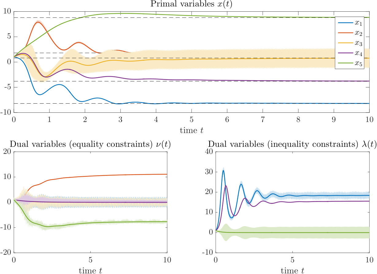
We can then follow the same procedure as discussed before to project on any P. Hall basis, where $\Phi$ now additionally includes the vector fields $h_{2,n+1}$ , $h_{n+1,n+3}$ , $h_{n+3,n+4}$ , and $h_{n+4,n+5}$ , and then apply the algorithm presented in Section A.5. The corresponding simulation results are depicted in Figure 5. As already indicated in Section 4.4, the nature of the approximating inputs produces heavy oscillations in the agents’ states. We next want to illustrate how a properly chosen filter as described in Section 4.4 can be used to dampen these oscillations while still maintaining the distributed structure. In this example, we assume that the low-pass filters $G_{x},G_{\nu},G_{\lambda}$ are of first order and take $G_{x}(s)=\tfrac{70}{s+70}$ , $G_{\nu}(s)=\tfrac{170}{s+170}$ , $G_{\lambda}(s)=\tfrac{170}{s+170}$ . We do not go through the calculations necessary to find distributed approximations of the filtered saddle-points dynamics since they literally follow the lines of the first part of the example. The corresponding simulation results are depicted in Figure 5. Compared to Figure 5, the trajectories of the distributed approximation show less oscillations which in turn also leads to an improved approximate solution of the distributed optimization problem. .

Refer to caption — Figure 5: Simulation results for the example of Section 5.2 with communication graph (b) given in Figure 4 without (top) and with additional filters (bottom). The thick lines depict the trajectories of the (non-distributed) saddle-point dynamics with initial condition $z(0)=\mathbf{1}\in\real^{15}$ , whereas the thinner oscillating lines depict the solution of the distributed approximation with the same initial condition $z^{\sigma}(0)=z(0)$ . Where no oscillating lines are visible, they are covered by the corresponding component of the solution $z(\cdot)$ . The dashed black lines indicate the optimal solution of the optimization problem given by $x^{\star}=[-8.2,\;1.8,\;0.8,\;-3.8,\;8.8]^{\top}$ . For both simulations the frequencies were chosen differently but according to some heuristics making sure that the minimally canceling property from Definition 4 is fulfilled. Further, we used $\sigma=1000$ .

6 Conclusion and outlook

We presented a new approach to distributed optimization problems where the communication topology is given by a directed graph. Our approach is based on a two-step procedure where in a first step first we derived suitable Lie bracket representations of saddle-point dynamics and then used Lie bracket approximations techniques from geometric control theory to obtain distributed control laws. While we limited ourselves to the class of convex problems with separable cost function and linear equality and inequality constraints that match the communication topology, the methodology is applicable to a much larger class of optimization problems including, for example, non-linear constraints, constraints not compatible with the graph structure or non-separable cost functions; we discuss in [18] how the rewriting procedure has to be adapted. Certainly, this generality comes with the cost of a possibly complex calculation of the approximating inputs; however, the strength of the presented approach is that it provides a unified framework for very general distributed optimization problems. Additionally, similar techniques can be applied to distributed control problems. We also presented a simplified algorithm for the design of approximating inputs that exploits the problem structure. Summarizing, the presented approach provides a systematic way to address distributed optimization problems under mild assumptions on the communication graph as well as the problem structure. We emphasize that, for practical implementations, there is still a long way to go. In particular, the highly oscillatory nature of the approximating inputs as well as time synchronization will be a major challenge. Apart from that, the design of suitable approximating inputs with improved transient and asymptotic behavior is complex and still an important issue to be addressed. While filters can be used as a simple remedy to this problem, there are also two other ways we plan to approach this problem: (1) altering the choice of admissible vector fields and (2) modifying the design of the approximating inputs including an optimal choice of parameters.

Acknowledgements

We thank Raik Suttner for his very valuable comments.

References

[1] S. Michalowsky, B. Gharesifard, and C. Ebenbauer, “A Lie bracket approximation approach to distributed optimization over directed graphs,” Automatica, 2019, accepted for publication.
[2] M. Geidl and G. Andersson, “Optimal power dispatch and conversion in systems with multiple energy carriers,” in Proc. 15th Power Systems Computation Conference (PSCC). Citeseer, 2005.
[3] S. Boyd, N. Parikh, E. Chu, B. Peleato, and J. Eckstein, “Distributed optimization and statistical learning via the alternating direction method of multipliers,” Foundations and Trends in Machine Learning, vol. 3, no. 1, pp. 1–122, 2011.
[4] F. Bullo, J. Cortés, and S. Martínez, Distributed Control of Robotic Networks, ser. Applied Mathematics Series. Princeton University Press, 2009.
[5] Z. Costello and M. Egerstedt, “The degree of nonholonomy in distributed computations,” in 53rd IEEE Conference on Decision and Control, 2014, pp. 6092–6098.
[6] M.-A. Belabbas, “Sparse stable systems,” Systems & Control Letters, vol. 62, no. 10, pp. 981–987, 2013.
[7] X. Chen, M. A. Belabbas, and T. Başar, “Controllability of formations over directed graphs,” in 2015 54th IEEE Conference on Decision and Control (CDC), 2015, pp. 4764–4769.
[8] B. Gharesifard, “Stabilization of bilinear sparse matrix control systems using periodic inputs,” Automatica, vol. 77, no. Supplement C, pp. 239 – 245, 2017.
[9] A. Nedić and A. Olshevsky, “Distributed optimization over time-varying directed graphs,” IEEE Transactions on Automatic Control, vol. 60, no. 3, pp. 601–615, 2015.
[10] D. Feijer and F. Paganini, “Stability of primal-dual gradient dynamics and applications to network optimization,” Automatica, vol. 46, no. 12, pp. 1974–1981, 2010.
[11] J. Wang and N. Elia, “A control perspective for centralized and distributed convex optimization,” in 2011 IEEE 50th Conference on Decision and Control and European Control Conference (CDC-ECC), 2011, pp. 3800–3805.
[12] H.-B. Dürr and C. Ebenbauer, “On a class of smooth optimization algorithms with applications in control,” IFAC Proceedings Volumes, vol. 45, no. 17, pp. 291–298, 2012, 4th IFAC Conference on Nonlinear Model Predictive Control.
[13] S. K. Niederländer and J. Cortés, “Distributed coordination for separable convex optimization with coupling constraints,” in 54th IEEE Conference on Decision and Control (CDC), Dec 2015, pp. 694–699.
[14] B. Gharesifard and J. Cortés, “Distributed continuous-time convex optimization on weight-balanced digraphs,” IEEE Transactions on Automatic Control, vol. 59, no. 3, pp. 781–786, 2014.
[15] B. Touri and B. Gharesifard, “Saddle-point dynamics for distributed convex optimization on general directed graphs,” in 2016 IEEE 55th Conference on Decision and Control (CDC), 2016, pp. 862–866.
[16] C. Ebenbauer, S. Michalowsky, V. Grushkovskaya, and B. Gharesifard, “Distributed optimization over directed graphs with the help of Lie brackets,” in Proc. 20th IFAC World Congress, 2017, pp. 15 908–15 913.
[17] S. Michalowsky, B. Gharesifard, and C. Ebenbauer, “Distributed extremum seeking over directed graphs,” in 2017 IEEE 56th Conference on Decision and Control (CDC), 2017, pp. 2095–2101.
[18] ——, “On the Lie bracket approximation approach to distributed optimization: Extensions and limitations,” in Proc. European Control Conf. (ECC), Limassol, Cyprus, 2018, pp. 119–124.
[19] N. Bourbaki, Lie Groups and Lie Algebras: Chapters 1–3, ser. Actualités scientifiques et industrielles. Hermann, 1998.
[20] N. Biggs, Algebraic graph theory. Cambridge University Press, 1993.
[21] J.-B. Hiriart-Urruty and C. Lemaréchal, Convex analysis and minimization algorithms I: Fundamentals. Springer science & business media, 2013, vol. 305.
[22] G. Wachsmuth, “On LICQ and the uniqueness of Lagrange multipliers,” Operations Research Letters, vol. 41, no. 1, pp. 78–80, 2013.
[23] H.-B. Dürr, “Constrained extremum seeking: A Lie bracket and singular perturbation approach,” PhD Thesis, University of Stuttgart, 2015.
[24] V. Grushkovskaya, A. Zuyev, and C. Ebenbauer, “On a class of generating vector fields for the extremum seeking problem: Lie bracket approximation and stability properties,” Automatica, vol. 94, pp. 151–160, 2018.
[25] T. H. Cormen, Introduction to algorithms. MIT press, 2009.
[26] W. Liu, “An approximation algorithm for nonholonomic systems,” SIAM Journal on Control and Optimization, vol. 35, no. 4, pp. 1328–1365, 1997.
[27] H. J. Sussmann and W. Liu, “Limits of highly oscillatory controls and the approximation of general paths by admissible trajectories,” in 30th IEEE Conference on Decision and Control. IEEE, 1991, pp. 437–442.
[28] W. Liu, “Averaging theorems for highly oscillatory differential equations and iterated Lie brackets,” SIAM journal on control and optimization, vol. 35, no. 6, pp. 1989–2020, 1997.
[29] C. Reutenauer, “Free Lie algebras,” Handbook of algebra, vol. 3, pp. 887–903, 2003.
[30] H.-B. Dürr, M. S. Stankovic, C. Ebenbauer, and K. H. Johansson, “Lie bracket approximation of extremum seeking systems,” Automatica, vol. 49, no. 6, pp. 1538–1552, 2013.
[31] S. Michalowsky and C. Ebenbauer, “The multidimensional n-th order heavy ball method and its application to extremum seeking,” in Proc. 53rd IEEE Conf. Decision and Control (CDC), Los Angeles, CA, USA, 2014, pp. 2660–2666.
[32] L. Bregman, “The relaxation method of finding the common point of convex sets and its application to the solution of problems in convex programming,” USSR computational mathematics and mathematical physics, vol. 7, no. 3, pp. 200–217, 1967.
[33] “The On-Line Encyclopedia of Integer Sequences, A000048,” https://oeis.org/A000048.
[34] “The On-Line Encyclopedia of Integer Sequences, A006788,” https://oeis.org/A006788.

Appendix A Appendix

A.1 Proof of Lemma 1

The proof follows a similar argument as the one in [23, Theorem 5.1.3]. First, using (13c), we have

\displaystyle\lambda_{i}(t)=\exp\big({\int_{0}^{t}\big(a_{i}x(\tau)-b_{i}\big)\mathrm{d}\tau}\big)\lambda_{i}(0),

(87)

for all $i=1,2,\dots,n$ ; hence, $\lambda_{i}(0)>0$ implies that $\lambda_{i}(t)>0$ , for all $t\geq 0$ , and consequently, the set $\mathcal{R}(\mathcal{M})$ is positively invariant w.r.t. (87). Let $(x^{\star},\nu^{\star},\lambda^{\star})$ be an arbitrary point in $\mathcal{M}$ . Consider the candidate Lyapunov function $V:\real^{n}\times\real^{n}\times{\mathbb{R}_{>0}}\to{\mathbb{R}_{\geq 0}}$ defined as

	$\displaystyle V(x,\nu,\lambda)$	$\displaystyle=\tfrac{1}{2}\\|x-x^{\star}\\|^{2}+\tfrac{1}{2}\\|\nu-\nu^{\star}\\|^{2}$
		$\displaystyle+\sum\limits_{i=1}^{n}(\lambda_{i}-{\lambda_{i}}^{\star})-\sum\limits_{i:\lambda_{i}^{\star}\neq 0}^{n}\lambda_{i}^{*}\ln(\tfrac{\lambda_{i}}{\lambda_{i}^{\star}}).$		(88)

We first observe that $V$ is positive definite with respect to $(x^{\star},\nu^{\star},\lambda^{\star})$ on $\mathcal{R}(\mathcal{M})$ , and that all the level sets are compact. To see this, note that according to [32, p. 207, eq. (1.5)], the function $D:{\mathbb{R}_{>0}^{n}}\times{\mathbb{R}_{>0}^{n}}\to\real$ defined as

	$\displaystyle D(\lambda^{\star},\lambda)$	$\displaystyle=\sum\limits_{i=1}^{n}\big(\lambda_{i}-\lambda_{i}^{\star}+\lambda_{i}^{\star}(\ln(\lambda_{i}^{\star})-\ln(\lambda_{i}))\big)$		(89)
		$\displaystyle=\sum\limits_{i=1}^{n}(\lambda_{i}-\lambda_{i}^{\star})-\sum\limits_{i:\lambda_{i}^{\star}\neq 0}^{n}\lambda^{\star}_{i}\ln(\tfrac{\lambda_{i}}{\lambda_{i}^{\star}})$		(90)

is positive for all $(\lambda^{\star},\lambda)\in{\mathbb{R}_{>0}^{n}}\times{\mathbb{R}_{>0}^{n}}$ and zero if and only if $\lambda=\lambda^{*}$ [32, Condition I.] and its level sets are compact [32, Condition V.]. Thus, with $V(x,\nu,\lambda)$ additionally being quadratic in $x$ and $\nu$ , positive definiteness and compactness of all level sets follows and hence $V$ is uniformly unbounded on $\mathcal{R}(\mathcal{M})$ . The derivative of $V$ along the trajectories of (13) is then given by

		$\displaystyle\dot{V}(x,\nu,\lambda)$		(91)
		$\displaystyle=-(x-x^{\star})^{\top}\big(\nabla F(x)+A^{\top}\nu+C^{\top}\lambda\big)$
		$\displaystyle+(\nu-\nu^{\star})^{\top}(Ax-b)$
		$\displaystyle-\sum\limits_{\begin{subarray}{c}i=1\\ i\notin\mathcal{I}_{\textup{eq}}\end{subarray}}^{n}\nu_{i}^{2}+\sum\limits_{i=1}^{n}\lambda_{i}({c}_{i}x-d_{i})-\sum\limits_{i:\lambda_{i}^{\star}\neq 0}^{n}\lambda_{i}^{\star}({c}_{i}x-d_{i})$
		$\displaystyle=-(x-x^{\star})^{\top}\nabla F(x)-\nu^{\top}\big(Ax-b-(Ax^{\star}-b)\big)$
		$\displaystyle-\lambda^{\top}\big({Cx-d-(Cx^{\star}-d)}\big)+(\nu-\nu^{\star})^{\top}(Ax-b)$
		$\displaystyle-\sum\limits_{\begin{subarray}{c}i=1\\ i\notin\mathcal{I}_{\textup{eq}}\end{subarray}}^{n}\nu_{i}^{2}+\sum\limits_{i=1}^{n}(\lambda_{i}-\lambda_{i}^{\star})({c}_{i}x-d_{i})+F(x)-F(x),$

Using strict convexity of $F$ , we now have that $-(x-x^{\star})^{\top}\nabla F(x)<F(x^{\star})-F(x)$ , for all $x\neq x^{\star}$ and hence we obtain for all $x\neq x^{\star}$

		$\displaystyle\dot{V}(x,\nu,\lambda)$		(92)
		$\displaystyle<F(x^{\star})-F(x)-\nu^{\top}\big(Ax-b-(Ax^{\star}-b)\big)$
		$\displaystyle-\lambda^{\top}\big(Cx-d-(Cx^{\star}-d)\big)+(\nu-\nu^{\star})^{\top}(Ax-b)$
		$\displaystyle-\sum\limits_{\begin{subarray}{c}i=1\\ i\notin\mathcal{I}_{\textup{eq}}\end{subarray}}^{n}\nu_{i}^{2}+\sum\limits_{i=1}^{n}(\lambda_{i}-{\lambda_{i}}^{\star})({c}_{i}x-d_{i})+F(x)-F(x)$
		$\displaystyle=L(x^{\star},\nu,\lambda)-L(x,\nu,\lambda)+L(x,\nu,\lambda)-L(x,\nu^{\star},\lambda^{\star})$
		$\displaystyle-\sum\limits_{\begin{subarray}{c}i=1\\ i\notin\mathcal{I}_{\textup{eq}}\end{subarray}}^{n}\nu_{i}^{2}$
		$\displaystyle=L(x^{\star},\nu,\lambda)-L(x,\nu^{\star},\lambda^{\star})-\sum\limits_{\begin{subarray}{c}i=1\\ i\notin\mathcal{I}_{\textup{eq}}\end{subarray}}^{n}\nu_{i}^{2}.$		(93)

Due to the saddle point property (12) the derivative of $V$ along the flow is strictly negative, for all $(x,\nu,\lambda)$ except for $(x,\nu,\lambda)\in\mathcal{M}$ ; thus, $(x^{\star},\nu^{\star},\lambda^{\star})$ is stable according to [23, Theorem 2.2.2]. This procedure can be repeated for any point $(x^{\star},\nu^{\star},\lambda^{\star})\in\mathcal{M}$ , hence $\mathcal{M}$ is stable. Let $L_{\textup{orig}}$ denote the Lagrangian associated to the original problem (4) and let $\mathcal{S}_{\textup{orig}}$ denote the corresponding set of saddle points. Observe that $L(x,\nu,\lambda)=L_{\textup{orig}}(x,\nu_{\mathcal{I}_{\textup{eq}}},\lambda_{\mathcal{I}_{\textup{ineq}}})-\sum_{{i=1,i\notin\mathcal{I}_{\textup{ineq}}}}^{n}\lambda_{i}d_{i}$ such that $\lambda_{i}^{\star}=0$ for all $i=1,2,\dots,n$ , $i\notin\mathcal{I}_{\textup{ineq}}$ , for any saddle point $(x^{\star},\nu^{\star},\lambda^{\star})$ of $L$ , since $d_{i}>0$ for $i=1,2,\dots,n$ , $i\notin\mathcal{I}_{\textup{ineq}}$ . Thus, the set of saddle points of $L$ is given by

	$\displaystyle\mathcal{S}=\{\penalty\$	$\displaystyle(x,\nu,\lambda)\in\real^{n}\times\real^{n}\times{\mathbb{R}_{\geq 0}^{n}}:$		(94)
		$\displaystyle(x,\nu_{\mathcal{I}_{\textup{eq}}},\lambda_{\mathcal{I}_{\textup{ineq}}})\in\mathcal{S}_{\textup{orig}},\lambda_{i}=0\text{ for }i\notin\mathcal{I}_{\textup{ineq}}\}$

and hence, $\mathcal{M}=\{(x,\nu,\lambda)\in\real^{n}\times\real^{n}\times\real^{n}:(x,\nu_{\mathcal{I}_{\textup{eq}}},\lambda_{\mathcal{I}_{\textup{ineq}}})\in\mathcal{S}\text{ and }\nu_{i}=0\text{ for }i\notin\mathcal{I}_{\textup{eq}},\lambda_{i}=0\text{ for }i\notin\mathcal{I}_{\textup{ineq}}\}$ . Since $\mathcal{S}_{\textup{orig}}$ is compact due to Assumption 2, the set $\mathcal{M}$ is compact as well. The same argument as the one in the proof of [23, Theorem 5.1.3] then yields that the set of saddle points is asymptotically stable with respect to the set of initial conditions $\mathcal{R}(\mathcal{M})$ .

A.2 Proof of Lemma 2

We prove the result by induction. For paths of the form $p_{i_{1}i_{2}}=\langle v_{i_{1}}|v_{i_{2}}\rangle$ , i.e., $\ell(p_{i_{1}i_{2}})=1$ , by (26) and (29) equation (31) follows immediately. Further we observe that the vector field (29) is admissible if $k_{1}\in\mathcal{I}(j),k_{2}\in\mathcal{I}(i)$ and $g_{ij}\neq 0$ , which is true since $p_{ij}$ is a path in $\mathcal{G}$ . Suppose now that the result holds for all paths $p$ with $\ell(p)\leq\bar{\ell}$ , $\bar{\ell}\geq 2$ . Let $p_{i_{1}i_{\ell}}=\langle v_{i_{1}}|v_{i_{2}}|\dots|v_{i_{k}}\rangle$ be any path with $\ell(p_{i_{1}i_{k}})=\bar{\ell}+1$ . Let further $q_{r}\in\mathrm{subpath}_{i_{1}\bullet}(p_{i_{1}i_{k}})$ be a subpath of $p_{i_{1}i_{k}}$ that ends at $v_{r}$ , $r=i_{2},i_{3},\dots,i_{k-1}$ . Then, since $\ell(q_{r})\leq\bar{\ell}$ , $\ell(q_{r}^{c})\leq\bar{\ell}$ , we have by (30) and the induction hypothesis

$\displaystyle R_{k_{1},k_{2}}(p_{i_{1}i_{k}}\big)(z)$	$\displaystyle=\big[R_{k_{1},s}(q_{r}^{c}),R_{s,k_{2}}(q_{r})\big](z)$
	$\displaystyle=\big[h_{k_{1},s},h_{s,k_{2}}\big](z)$
	$\displaystyle=e_{k_{2}}e_{s}^{\top}z_{k_{1}}e_{s}-e_{s}e_{k_{1}}^{\top}z_{s}e_{k_{2}}$
	$\displaystyle=z_{k_{1}}e_{k_{2}},$	(95)

where $s\in\mathcal{I}(\textup{tail}(q_{r}))$ and where we have used that $k_{1}\neq k_{2}$ . This proves (31). Further, if $k_{1}\in\mathcal{I}\big(\textup{tail}(p_{i_{1}i_{k}})\big)$ , i.e., $k_{1}\in\mathcal{I}\big(\textup{tail}(q_{r}^{c})\big)$ , then, by the induction hypothesis and with $s\in\mathcal{I}(\textup{tail}(q_{r}))=\mathcal{I}(\textup{head}(q_{r}^{c}))$ , $R_{k_{1},s}(q_{r}^{c})$ is a Lie bracket of admissible vector fields. Similarly, if $k_{2}\in\mathcal{I}\big(\textup{head}(p_{i_{1}i_{k}})\big)$ , by the induction hypothesis and with $s\in\mathcal{I}(\textup{tail}(q_{r}))$ , also $R_{s,k_{2}}(q_{r})$ is a Lie bracket of admissible vector fields. Thus, $R_{k_{1},k_{2}}(p_{i_{1}i_{k}}\big)$ is a Lie bracket of admissible vector fields as well, which concludes the proof.

A.3 Proof of Lemma 3

We first observe first that (38) is the same as (29), (30) with a special choice of the subpath as well as an additional projection with the property $\textup{proj}_{{\mathbb{P}}}\big(B\big)(z)=B(z)$ for all $z\in\real^{3n}$ . Hence, it immediately follows that $\tilde{R}_{k_{1},k_{2}}(p_{i_{1}i_{r}})(z)=R_{k_{1},k_{2}}(p_{i_{1}i_{r}})(z)$ . In the same manner, we also have that

\displaystyle\delta\big(\tilde{R}_{k_{1},k_{2}}(p_{i_{1}i_{r}})\big)=\delta\big(R_{k_{1},k_{2}}(p_{i_{1}i_{r}})\big)=\ell(p_{i_{1}i_{r}}).

(96)

We show the second part by induction. First observe that for paths $p_{i_{1}i_{r}}$ with $\ell(p_{i_{1}i_{r}})=1$ it is clear that $\tilde{R}_{k_{1},k_{2}}(p_{i_{1}i_{r}})\in\mathbb{P}$ since $R_{k_{1},k_{2}}(p_{i_{1}i_{r}})$ is an admissible vector field by Lemma 2 and all admissible vector fields are in $\mathbb{P}$ . Further, for paths $p_{i_{1}i_{r}}$ with $\ell(p_{i_{1}i_{r}})\in\{2,3,4,6\}$ it also follows from the definition of the projection that $\tilde{R}_{k_{1},k_{2}}(p_{i_{1}i_{r}})\in\mathbb{P}$ . Suppose now that the result holds true for all paths $p$ with $\ell(p)=\bar{\ell}$ , where $\bar{\ell}\geq 2$ , and consider a path $p_{i_{1}i_{r}}$ with $\ell(p_{i_{1}i_{r}})=\bar{\ell}+1$ . Observe that all subbrackets of $\tilde{R}_{k_{1},k_{2}}(p_{i_{1}i_{r}})$ are in $\mathbb{P}$ by the induction hypothesis and hence, by [PH3], [PH4][PH4.a], [PH4][PH4.b], we have ${B}:=\tilde{R}_{k_{1},k_{2}}(p_{i_{1}i_{r}})\in\mathbb{P}$ if

	$\displaystyle\delta\big(\textup{left}({B})\big)$	$\displaystyle<\delta\big(\textup{right}({B})\big)$		(97)
	$\displaystyle\delta\big(\textup{left}(\textup{right}({B}))\big)$	$\displaystyle<\delta\big(\textup{left}({B})\big);$		(98)

we will show next that these conditions are fulfilled for the above choice of subpaths. By (38) and (40) we have

	$\displaystyle\delta\big(\textup{right}(\tilde{R}_{k_{1},k_{2}}(p_{i_{1}i_{r}}))\big)$	$\displaystyle=\delta\big(\tilde{R}_{s,k_{2}}(q)\big)=\ell(q)$
	$\displaystyle\delta\big(\textup{left}(\tilde{R}_{k_{1},k_{2}}(p_{i_{1}i_{r}}))\big)$	$\displaystyle=\delta\big(\tilde{R}_{k_{1},s}(q^{c})\big)=\ell(p_{i_{1}i_{r}})-\ell(q).$

Since $\lfloor\tfrac{a}{b}\rfloor\geq\tfrac{a-b+1}{b}$ , for all $a\in\mathbb{Z},b\in{\rm Nature}$ , we infer

\displaystyle\ell(q)

\displaystyle=\theta(p_{i_{1}i_{r}})-1\geq\tfrac{\ell(p_{i_{1}i_{r}})+1}{2},

(99)

for $\ell(p_{i_{1}i_{r}})\geq 5$ , and hence we obtain

	$\displaystyle\delta\big(\textup{right}(\tilde{R}_{k_{1},k_{2}}(p_{i_{1}i_{r}}))\big)-\delta\big(\textup{left}(\tilde{R}_{k_{1},k_{2}}(p_{i_{1}i_{r}}))\big)$
	$\displaystyle\geq\ell(p_{i_{1}i_{r}})+1-\ell(p_{i_{1}i_{r}})>0.$		(100)

Thus, (97) holds. For (98), we first note that

\displaystyle\delta\big(\textup{left}(\textup{right}(\tilde{R}_{k_{1},k_{2}}(p_{i_{1}i_{r}})))\big)

\displaystyle=\delta\big(\textup{left}(\tilde{R}_{s,k_{2}}(q))\big)\hskip-10.00002pt

(101)

and, since $\textup{left}(\tilde{R}_{s,k_{2}}(q))\in\mathbb{P}$ by the induction hypothesis, it is $\delta\big(\textup{left}(\tilde{R}_{s,k_{2}}(q))\big)\leq\delta\big(\textup{right}(\tilde{R}_{s,k_{2}}(q))\big)=\ell(q)-\delta\big(\textup{left}(\tilde{R}_{s,k_{2}}(q))\big)$ according to [PH4][PH4.a]. Hence, we obtain

\displaystyle\delta\big(\textup{left}(\textup{right}(\tilde{R}_{k_{1},k_{2}}(p_{i_{1}i_{r}})))\big)\leq\tfrac{\ell(q)}{2}.

(102)

As a result, (98) is fulfilled when

\displaystyle\tfrac{\ell(q)}{2}\leq\ell(p_{i_{1}i_{r}})-\ell(q).

(103)

We now compute

\displaystyle\tfrac{3}{2}\ell(q)

\displaystyle=\tfrac{3}{2}\lfloor\tfrac{\ell(p_{i_{1}i_{r}})}{2}\rfloor+\tfrac{3}{2}\leq\tfrac{3}{4}\ell(p_{i_{1}i_{r}})+\tfrac{3}{2}\leq\ell(p_{i_{1}i_{r}}),

for $\ell(p_{i_{1}i_{r}})\geq 6$ ; for $\ell(p_{i_{1}i_{r}})=5$ , we have that $\tfrac{3}{2}\ell(q)=\tfrac{9}{2}<\ell(p_{i_{1}i_{r}})$ , thus (103) holds for all considered $p_{i_{1}i_{r}}$ which proves that (98) holds; this concludes the proof.

A.4 Proof of Proposition 2

It is clear that (55) holds for $\ell(p_{ij})=2$ , since $\tilde{R}_{r+j,i}(p_{ij})$ is a bracket of degree two, i.e., a bracket of the form $[\phi_{k_{1}},\phi_{k_{2}}]$ , $k_{1}\neq k_{2}$ , such that

\displaystyle{E_{\textup{proj}_{{\mathbb{P}}}([\phi_{k_{1}},\phi_{k_{2}}])}}

\displaystyle=\begin{cases}[\phi_{k_{1}},\phi_{k_{2}}]\text{ if }k_{1}<k_{2}\\ [\phi_{k_{2}},\phi_{k_{1}}]\text{ if }k_{2}<k_{1}.\end{cases}

(104)

Consider now a path $p_{i_{1}i_{4}}=\langle v_{i_{1}}|v_{i_{2}}|v_{i_{3}}|v_{i_{4}}\rangle$ , $i_{1}\neq i_{2}\neq i_{3}\neq i_{4}$ , i.e., $\ell(p_{i_{1}i_{4}})=3$ . Then

		$\displaystyle\tilde{R}_{r+i_{4},i_{1}}(p_{i_{1}i_{4}})$
		$\displaystyle=\textup{proj}_{{\mathbb{P}}}\big(R_{r+i_{4},i_{1}}(p_{i_{1}i_{4}})\big)$
		$\displaystyle=\textup{proj}_{{\mathbb{P}}}\big(\big[h_{r+i_{4},r+i_{3}},[h_{r+i_{3},r+i_{2}},h_{r+i_{2},i_{1}}]\big]\big)$
		$\displaystyle=-\big[h_{r+i_{4},r+i_{3}},[h_{r+i_{2},i_{1}},h_{r+i_{3},r+i_{2}}]\big],$		(105)

where we have used the assumption on the ordering of the P. Hall basis. The only equivalent bracket in $\mathbb{P}$ is then given by ${B}=\big[h_{r+i_{3},r+i_{2}},[h_{r+i_{2},i_{1}},h_{r+i_{4},r+i_{3}}]\big]$ , but we have that $B(z)\equiv 0$ , since

		$\displaystyle[h_{r+i_{2},i_{1}},h_{r+i_{4},r+i_{3}}](z)$
		$\displaystyle=e_{r+i_{3}}e_{r+i_{4}}^{\top}e_{i_{1}}z_{r+i_{2}}-e_{i_{1}}e_{r+i_{2}}^{\top}e_{r+i_{3}}z_{+i_{2}}=0.$		(106)

Thus, the claim follows.

A.5 A simplified algorithm for the construction of approximating sequences

$\delta(B)$	$2$	$3$	$4$	$5$	$6$	$7$	$8$	$9$	$10$	$11$	$12$	$13$	$14$	$15$	$16$	$17$
$\|{E_{B,\textup{full}}}\|$	$1$	$2$	$3!$	$4!$	$5!$	$6!$	$7!$	$8!$	$9!$	$10!$	$11!$	$12!$	$13!$	$14!$	$15!$	$16!$
$\|{E_{B}}\|$	$1$	$1$	$2$	$3$	$5$	$9$	$16$	$28$	$51$	$93$	$170$	$315$	$585$	$1089$	$2048$	$3855$

Table 1: A comparison of

|{E_{B,\textup{full}}}|

and

|{E_{B}}|

for a specific choice of the P. Hall basis that fulfills the assumptions as in Proposition 2. The numbers were obtained by symbolically computing the resulting vector fields using a computer algebra system. Interestingly, the sequence of

|{E_{B}}|

has two matching sequences [33] and [34] except for the value for

\delta(B)=15

which should be 1091 or 1092, thus we conjecture that these sequences are a good upper bound for

|{E_{B}}|

Our objective in this section is to provide a modified version of the construction procedure from [26] using the structural properties of the problem at hand, which leads to considerable simplifications. Given the scopes of this paper and the complicated nature of the subject, we do not discuss this algorithm in detail; we refer the reader to the supplementary material of the present manuscript, as well as the original work [26]. We first provide a formal definition of the already mentioned equivalence relation on the set of Lie brackets:

Definition 3 (Equivalent brackets).

Let $\mathcal{PH}=(\mathbb{P},\prec)$ be a P. Hall basis of $\Phi=\{\phi_{1},\dots,\phi_{M}\}$ and let $\delta_{k}(B)$ denote the degree of the vector field $\phi_{k}$ in the bracket $B\in\mathcal{PH}$ . We say that two brackets $B_{1},B_{2}\in{\mathbb{P}}$ are equivalent, denoted by $B_{1}\sim B_{2}$ , if $\delta_{k}(B_{1})=\delta_{k}(B_{2})$ for all $k=1,\dots,M$ . $\bullet$

For a given set of brackets $\mathbb{P}$ , we then denote by $E_{B}=\{\tilde{B}\in\mathbb{P}:\tilde{B}\sim B\}$ the equivalence class corresponding to the bracket $B\in\mathbb{P}$ . Note that, by definition of the equivalence relation, all brackets contained in an equivalence class $E=\{B_{1},B_{2},\dots,B_{r}\}$ , $r\in\mathbb{N}_{>0}$ , have the same degree and we hence let $\delta(E)=\delta(B_{k})$ , $k\in\{1,2,\dots,r\}$ , denote the degree of the equivalence class. For the construction of the sets of frequencies, we also need the following two definitions:

Definition 4 (Minimally canceling).

A set $\Omega=\{\omega_{1},\dots,\omega_{m}\}$ is called minimally canceling if for each collection of integers $\{y_{i}\}_{i=1}^{m}$ , such that $\sum_{k=1}^{m}|y_{k}|\leq m$ we have $\sum_{k=1}^{m}y_{k}\omega_{k}=0$ if and only if all $y_{k}$ are equal. $\bullet$

Definition 5 (Independent collection).

A finite collection of sets $\{\Omega_{\lambda}\}_{\lambda=1}^{N}$ , where $\Omega_{\lambda}=\{\omega_{\lambda,1},\omega_{\lambda,2}\dots,\omega_{\lambda,M_{\lambda}}\}$ , is called independent if the followings hold:

1.

the sets $\Omega_{\lambda}$ are pairwise disjoint, and

for each collection of integers $\{y_{i,k}\}_{i=1}^{N}$ , $k\penalty\ =\penalty\ 1,\dots,M_{i}$ , such that

\displaystyle\sum\limits_{i=1}^{N}\sum\limits_{k=1}^{M_{i}}y_{i,k}\omega_{i,k}=0\quad\text{and}\quad\sum\limits_{i=1}^{N}\sum\limits_{k=1}^{M_{i}}|y_{i,k}|\leq\sum\limits_{i=1}^{N}M_{i}

we have

\displaystyle\sum\limits_{k=1}^{M_{i}}y_{i,k}\omega_{i,k}=0,

(107)

for each $i=1,\dots,N$ . $\bullet$

Consider now an extended system of the form

\displaystyle\dot{z}=f_{0}(z)+\sum\limits_{\begin{subarray}{c}B\in\mathcal{B}\\ \delta(B)\geq 2\end{subarray}}v_{B}B(z),

(108)

where $f_{0}:\real^{N}\to\real^{N}$ , $\mathcal{B}\subset\mathbb{P}$ , $\mathcal{B}$ finite, for some P. Hall basis $\mathcal{PH}(\Phi)=(\mathbb{P},\prec)$ , $\Phi=\{\phi_{1},\phi_{2},\dots,\phi_{M}\}$ , $\phi_{k}:\real^{N}\to\real^{N}$ , $f_{0},\phi_{k}$ sufficiently smooth, $v_{B}\in\real\setminus\{0\}$ and $B(z)\not\equiv 0$ for all $B\in\mathcal{B}$ . Suppose that for any $B\in\mathcal{B}$ , we have that $\delta_{k}(B)\in\{0,1\}$ , $k=1,2,\dots,M$ . Consider the system

\displaystyle\dot{X}^{\sigma}=f_{0}(X^{\sigma})+\sum\limits_{k=1}^{M}\phi_{k}(X^{\sigma})U_{k}^{\sigma}(t).

(109)

The following algorithm allows to compute suitable input functions $U_{k}^{\sigma}$ such that the solutions of (109) uniformly converge to those of (108) with increasing $\sigma$ . It should as well be mentioned that we also provide an exemplary implementation of the algorithm in Matlab in the supplementary material.

Algorithm

Step 1 (Determining the equivalence classes): For all $B\in\mathcal{B}$ , determine the associated (reduced) equivalence class

	$\displaystyle{E_{B}}$	$\displaystyle=\{\tilde{B}\in{\mathbb{P}}:\tilde{B}\sim B,\tilde{B}(z)\not\equiv 0\}$
		$\displaystyle=\{\tilde{B}_{E,1},\tilde{B}_{E,2},\dots,\tilde{B}_{E,\|E(B)\|}\},$

and let $\mathcal{E}=\{{E_{B}},B\in\mathcal{B}\}$ . For each $B\in\mathbb{P}$ , set

\displaystyle\tilde{v}_{B}=\begin{cases}v_{B}&\text{if }B\in\mathcal{B}\\ 0&\text{otherwise.}\end{cases}

Step 2 (Determining the frequencies): For all $E\in\mathcal{E}_{2}:=\{E\in\mathcal{E}:\delta(E)=2\}$ , choose $|\mathcal{E}_{2}|$ distinct frequencies $\omega_{E}\in\real\setminus\{0\}$ , and for all $E\in\mathcal{E}$ , $\delta(E)\geq 3$ choose ${M}|E|$ sets

	$\displaystyle\Omega_{E,\rho,k}^{+}$	$\displaystyle=\begin{cases}{\{\omega_{E,\rho,k}\}}&\text{if }\delta_{k}(E)=1\\ \emptyset&\text{if }\delta_{k}(E)=0\end{cases}$
	$\displaystyle\Omega_{E,\rho,k}^{-}$	$\displaystyle=-\Omega_{{E},\rho,k}^{+},$

$\omega_{E,\rho,k}\in\real\setminus\{0\}$ , $k=1,\dots,M$ , $\rho=1,\dots,{|E|}$ , such that

1.

For each $E\in\mathcal{E}$ , $\delta(E)\geq 3$ , and each $\rho=1,\dots,|E|$ , the set $\Omega^{+}_{E,\rho}=\bigcup_{k=1}^{M}\Omega_{E,\rho,k}^{+}$ is minimally canceling.

The collection of sets

\displaystyle\Big\{\big\{\omega_{E},-\omega_{E}\big\}_{E\in\mathcal{E}_{2}},\big\{\Omega^{+}_{E,\rho}\cup\Omega^{-}_{E,\rho}\big\}_{\begin{subarray}{c}E\in\mathcal{E},\delta(E)\geq 3,\\ \rho=1,\dots,{|E|}\end{subarray}}\Big\}

is independent.

Step 3 (Calculating the auxiliary matrix $\Xi_{E}$ ): For all $E\in\mathcal{E}$ with $\delta(E)\geq 3$ , compute

\displaystyle\Xi_{E}=\begin{bmatrix}\xi_{\tilde{B}_{E,1},1}^{+}&\xi_{\tilde{B}_{E,1},2}^{+}&\dots&\xi_{\tilde{B}_{E,1},|E|}^{+}\\ \xi_{\tilde{B}_{E,2},1}^{+}&\xi_{\tilde{B}_{E,2},2}^{+}&\dots&\xi_{\tilde{B}_{E,2},|E|}^{+}\\ \vdots&\vdots&\ddots&\vdots\\ \xi_{\tilde{B}_{E,|E|},1}^{+}&\xi_{\tilde{B}_{E,|E|},2}^{+}&\dots&\xi_{\tilde{B}_{E,|E|},|E|}^{+}\end{bmatrix},

where, for any $B\in E$ , we let

\displaystyle\xi_{B,\rho}^{+}

\displaystyle=\hat{g}_{B}(\omega_{E,\rho,\theta_{B}(1)},\omega_{E,\rho,\theta_{B}(2)},\dots,\omega_{E,\rho,\theta_{B}(\delta(B))}),

with $\theta_{B}(i)=k$ if the $i$ th vector field in $B$ is $\phi_{k}$ and where $\hat{g}_{B}:\real^{\delta(B)}\to\real$ is defined as follows:

•

If $\delta(B)=1$ , then $\hat{g}_{B}(\tilde{\omega}_{1})=1.$

•

If $B=[B_{1},B_{2}]$ , then

		$\displaystyle\hat{g}_{B}(\tilde{\omega}_{1},\tilde{\omega}_{2},\dots,\tilde{\omega}_{\delta(B)})=\frac{\hat{g}_{B_{1}}(\tilde{\omega}_{1},\tilde{\omega}_{2},\dots,\tilde{\omega}_{\delta(B_{1})})}{\sum_{i=1}^{\delta(B_{1})}\tilde{\omega}_{i}}$
		$\displaystyle\times\;\hat{g}_{B_{2}}(\tilde{\omega}_{\delta(B_{1})+1},\tilde{\omega}_{\delta(B_{1})+2},\dots,\tilde{\omega}_{\delta(B_{1})+\delta(B_{2})}).$

Step 4 (Calculating the input coefficients): For all $E\in\mathcal{E}$ with $\delta(E)=2$ , i.e., $E(B)=\{B\}=\big[\phi_{k_{1}},\phi_{k_{2}}\big]$ , set

	$\displaystyle\eta_{E,k_{1}}(\omega_{E})$	$\displaystyle=\mathrm{i}\tfrac{1}{\beta_{E}}\text{sign}(\tilde{v}_{B}\omega_{E})\sqrt{\tfrac{1}{2}\|\tilde{v}_{B}\omega_{E}\|}$
	$\displaystyle\eta_{E,k_{2}}(\omega_{E})$	$\displaystyle=\beta_{E}\sqrt{\tfrac{1}{2}\|\tilde{v}_{B}\omega_{E}\|},$

where $\beta_{E}\neq 0$ . For all $E\in\mathcal{E}$ with $\delta(E)\geq 3$ let²² 2 We tacitly assume here that $\Xi_{E}$ is invertible. It has been shown in [26] that there always exists a choice of frequencies such that the corresponding matrix obtained when using “full” equivalence classes is invertible; however, it is not clear whether this also holds in the case of reduced equivalence classes where $\Xi_{E}$ is a submatrix obtained from the general one by removing several rows and columns.

\displaystyle\begin{bmatrix}\gamma_{E,1}\\ \gamma_{E,2}\\ \smash[t]{\vdots}\\[-5.0pt] \gamma_{E,|E|}\end{bmatrix}=\Xi_{E}^{-1}\begin{bmatrix}\tilde{v}_{\tilde{B}_{E,1}}\\ \tilde{v}_{\tilde{B}_{E,2}}\\ \smash[t]{\vdots}\\[-5.0pt] \tilde{v}_{\tilde{B}_{E,|E|}}\end{bmatrix}

and compute $\eta_{E}(\omega)$ as follows:

•

If $\delta(E)$ is odd, for each $\rho=1,\dots,|E|$ , take

$\displaystyle\eta_{E}(\omega)=\beta_{E,\omega}\big(\tfrac{1}{2}\gamma_{E,\rho}\mathrm{i}^{\delta(E)-1}\big)^{\tfrac{1}{\delta(E)}}$

for all $\omega\in\Omega_{E,\rho}^{+}$ , and

•

if $\delta(E)$ is even, for each $\rho=1,\dots,|E|$ , take

\displaystyle\eta_{E}(\tilde{\omega})

\displaystyle=\mathrm{i}\beta_{E,{\tilde{\omega}}}\text{sign}(\gamma_{E,\rho}(t)\mathrm{i}^{\delta(E)-2})\left|\tfrac{1}{2}\gamma_{E,\rho}(t)\mathrm{i}^{\delta(E)-2}\right|^{\tfrac{1}{\delta(E)}}

for some $\tilde{\omega}\in\Omega_{E,\rho}^{+}$ and

\displaystyle\eta_{E}(\omega)

\displaystyle=\beta_{E,\omega}\left|\tfrac{1}{2}\gamma_{E,\rho}(t)\mathrm{i}^{\delta(E)-2}\right|^{\tfrac{1}{\delta(E)}}

for all $\omega\in\Omega_{E,\rho}^{+}\setminus\{\tilde{\omega}\}$ .

In both cases $\beta_{E,\omega}\in\real$ can be chosen freely such that it fulfills $\prod_{\omega\in\Omega_{E,\rho}^{+}}\beta_{E,\omega}=1$ .
Step 5 (Calculating the approximating inputs): Compute the input according to $U_{k}^{\sigma}(t)=\sum_{E\in\mathcal{E}}U_{k,E}^{\sigma}(t)$ with $U_{k,E}^{\sigma}:\real\to\real$ being defined as follows:

•

If $\delta_{k}(E)=0$ : $U_{k,E}^{\sigma}(t)=0$ .
•

If $\delta(E)=2,\delta_{k}(E)=1$ :

$\displaystyle U_{k,E}^{\sigma}(t)=2\sqrt{\sigma}\text{Re}\big(\eta_{E,k}(\omega_{E})e^{\mathrm{i}\sigma\omega_{E}t}\big).$

•

If $\delta(E)=N$ , $\delta_{k}(E)=1$ :

\displaystyle U_{k,E}^{\sigma}(t)=2\sigma^{\tfrac{N-1}{N}}\sum\limits_{\rho=1}^{|E|}\text{Re}\big(\eta_{E}(\omega_{E,\rho,k})e^{\mathrm{i}\sigma\omega t}\big).

Note that this algorithm is a reformulation of the one presented in [26] (see the supplements of this manuscript for a derivation) exploiting two structural properties of the problem at hand: (1) each $B\in\mathcal{B}$ fulfills $\delta_{k}(B)\in\{0,1\}$ for all $k=1,2,\dots,M$ and (2) a large number of the equivalent brackets evaluate to zero (see Table 1). Note that (1) simplifies the calculation of $\xi^{+}_{B,\rho}$ in step 3 and (2) reduces the cardinality of each ${E_{B}}$ in step 1, where usually the full equivalence class ${E_{B,\textup{full}}}=\{\tilde{B}\in\mathcal{B}:\tilde{B}\sim B\}$ is used, thus leading to a reduction of the dimension of $\Xi_{E}$ in step 3 and hence also simplifying step 4. In fact, we can derive the following result on the equivalent brackets:

Lemma 4.

Consider a graph $\mathcal{G}=(\mathcal{V},\mathcal{E})$ of $n$ nodes. Let $p_{i_{1}i_{r}}=(v_{i_{1}},v_{i_{2}},\dots,v_{i_{r}})$ be the shortest path between $v_{i_{1}}$ and $v_{i_{r}}$ , $v_{i_{k}}\in\mathcal{V}$ for $k=1,2,\dots,r$ , $r\geq 3$ . Let $\Phi=\{\phi_{a_{1}},\phi_{a_{2}},\dots,\phi_{a_{r-1}}\}$ be a set of vector fields with

\displaystyle\phi_{a_{j}}\in\{h_{k_{1},k_{2}}:k_{1}\in\mathcal{I}(i_{j+1}),k_{2}\in\mathcal{I}(i_{j})\},

(110)

for $j=1,2,\dots,r-1$ . Denote some given P. Hall basis of $\Phi$ by $\mathcal{PH}(\Phi)=(\mathbb{P},\prec)$ . Let $B\in\mathbb{P}$ and suppose that $\delta_{a_{j}}(B)\in\{0,1\}$ for $j=1,2,\dots,r-1$ . Define $\mathcal{J}(B)=\{j=1,2,\dots,r-1:\delta_{a_{j}}(B)=1\}$ and further denote

\displaystyle j_{\textup{min}}(B)=\min\limits_{j\in\mathcal{J}(B)}\{j\},\quad j_{\textup{max}}(B)={\max\limits_{j\in\mathcal{J}(B)}\{j\}}.

(111)

Then, if $\mathcal{J}(B)$ is a connected set, i.e., $\mathcal{J}(B)=\{j_{\textup{min}}(B),j_{\textup{min}}(B)+1,\dots,j_{\textup{min}}(B)+\delta(B)-1\}$ and $j_{\textup{max}}(B)=j_{\textup{min}}(B)+\delta(B)-1$ , for any $k_{1}\in\mathcal{I}(i_{j_{\textup{max}}(B)+1})$ , $k_{2}\in\mathcal{I}(i_{j_{\textup{min}}(B)})$ and for all $z\in\real^{3n}$ , we have that

\displaystyle B(z)=\pm h_{k_{1},k_{2}}(z)\quad\text{or}\quad B(z)=0.

(112)

If $\mathcal{J}(B)$ is not a connected set, we have $B(z)=0$ for all $z\in\real^{3n}$ . $\bullet$

Proof.

We prove this result by induction. Suppose first that $\delta(B)=1$ . Then $\mathcal{J}(B)=\{j_{\textup{min}}\}=\{j_{\textup{max}}\}$ , which means it has only one element. Hence, the claim is obviously true. Since the case of $\mathcal{J}(B)$ not being a connected set does not appear for $\delta(B)=1$ , we also look at $\delta(B)=2$ . Let $\mathcal{J}(B)=\{j_{1},j_{2}\}$ , $j_{1}\neq j_{2}$ . Observe that, for all $j_{1},j_{2}=1,2,\dots,r-1$ , $j_{1}\neq j_{2}$ , and $j_{1}\leq r-2$ (or $j_{2}\leq r-1$ ), we have

$\displaystyle B(z)$	$\displaystyle=[\phi_{a_{j_{1}}},\phi_{a_{j_{2}}}](z)$
	$\displaystyle=[h_{k_{1},k_{2}},h_{k_{3},k_{4}}](z)$
	$\displaystyle=[z_{k_{1}}e_{k_{2}},z_{k_{3}}e_{k_{4}}]$
	$\displaystyle=e_{k_{4}}e_{k_{3}}^{\top}e_{k_{2}}z_{k_{1}}-e_{k_{2}}e_{k_{1}}^{\top}e_{k_{4}}z_{k_{3}},$	(113)

where $k_{1}\in\mathcal{I}(i_{j_{1}+1}),k_{2}\in\mathcal{I}(i_{j_{1}}),k_{3}\in\mathcal{I}(i_{j_{2}+1}),$ and $k_{4}\in\mathcal{I}(i_{j_{2}})$ . We then compute

\displaystyle[\phi_{a_{j_{1}}},\phi_{a_{j_{2}}}](z)

\displaystyle=\begin{cases}z_{k_{1}}e_{k_{4}}&\text{if }k_{2}=k_{3}\\ -z_{k_{3}}e_{k_{2}}&\text{if }k_{1}=k_{4}\\ 0&\text{otherwise}.\end{cases}

(114)

Note that $k_{2}=k_{3}$ only if $i_{j_{1}}=i_{j_{2}+1}$ , i.e., $j_{1}=j_{2}+1=j_{\textup{max}}$ , $j_{\textup{min}}=j_{2}$ , and $k_{1}=k_{4}$ only if $i_{j_{2}}=i_{j_{1}+1}$ , i.e., $j_{2}=j_{1}+1=j_{\textup{max}}$ , $j_{1}=j_{\textup{min}}$ ; hence $B(z)$ is non-zero only if $\mathcal{J}(B)=\{j_{1},j_{2}\}$ is connected, which proves that the claim is true for $\delta(B)=2$ . Note also that the case $k_{1}=k_{4},k_{2}=k_{3}$ cannot occur since $j_{1}\neq j_{2}$ . The second claim (112) follows immediately from these considerations. To proceed with our induction argument, suppose now that the claim is true for all $B\in\mathbb{P}$ that fulfill the assumptions with $\delta(B)\leq{\delta}^{*}$ , $\delta^{*}\leq r-1$ . Consider now some $B\in\mathbb{P}$ with $\delta(B)=\delta^{*}+1>2$ . Every $B$ can be written as $B=[B_{1},B_{2}]$ , where $\delta(B_{1}),\delta(B_{2})\leq\delta^{*}$ . Let $\mathcal{J}(B)=\{j_{1},j_{2},\dots,j_{\delta(B)}\}$ and assume, without loss of generality, that $j_{k}<j_{k+1}$ , for all $k=1,\dots,\delta(B)-1$ . By the induction hypothesis, $B_{1}(z)$ and $B_{2}(z)$ are non-zero only if $\mathcal{J}(B_{1})$ and $\mathcal{J}(B_{2})$ are both connected sets. Since $\mathcal{J}(B_{2})=\mathcal{J}(B)\setminus\mathcal{J}(B_{1})$ this is the case if and only if

	$\displaystyle\mathcal{J}(B_{1})$	$\displaystyle=\begin{cases}\{j_{1},j_{2},\dots,j_{\delta(B_{1})}\}\quad\mathrm{or}\\ \{j_{\delta(B)-\delta(B_{1})+1},j_{\delta(B)-\delta(B_{1})+2},\dots,j_{\delta(B)}\}\end{cases}$
		$\displaystyle=\begin{cases}\{j_{1},j_{1}+1,\dots,j_{1}+\delta(B_{1})-1\},\quad\mathrm{or}\\ \{j_{\delta(B)-\delta(B_{1})+1},j_{\delta(B)-\delta(B_{1})+1}+1,\dots,\\ \qquad\qquad\quad j_{\delta(B)-\delta(B_{1})+1}+\delta(B_{1})-1\}.\end{cases}$

We only consider the first case here, since the second case can be treated analogously. Using the first equality above, for $k_{1}\in\mathcal{I}(i_{j_{1}+\delta(B_{1})}),k_{2}\in\mathcal{I}(i_{j_{1}})$ , and $k_{3}\in\mathcal{I}(i_{j_{\delta(B)}+1}),k_{4}\in\mathcal{I}(i_{j_{\delta(B_{1})+1}})$ , we have by the induction hypothesis that

	$\displaystyle B_{1}(z)=\pm h_{k_{1},k_{2}}(z)\quad$	$\displaystyle\text{or}\quad B_{1}(z)=0$		(115)
	$\displaystyle B_{2}(z)=\pm h_{k_{3},k_{4}}(z)\quad$	$\displaystyle\text{or}\quad B_{2}(z)=0.$		(116)

Obviously, following our previous calculations, $[B_{1},B_{2}]$ is non-zero only if $k_{2}=k_{3}$ , meaning that $j_{1}=j_{\delta(B)}+1$ , or if $k_{1}=k_{4}$ , meaning that $j_{1}+\delta(B_{1})=j_{\delta(B_{1})+1}$ . The first case cannot occur, since $\delta(B)>2$ and $j_{k+1}>j_{k}$ ; the second case holds true if and only if $\mathcal{J}(B)$ is connected, thus showing that $B(z)$ is non-zero only if $\mathcal{J}(B)$ is connected. To show that (112) holds, consider the case that $\mathcal{J}(B)$ is connected, i.e., $\mathcal{J}(B)=\{j_{1},j_{1}+1,\dots,j_{1}+\delta(B)\}$ , $j_{\textup{min}}(B)=j_{1}$ , $j_{\textup{max}}(B)=j_{1}+\delta(B)$ , and $k_{1}=k_{4}$ . Then, following the same arguments as before, we have that $B(z)=\pm h_{k_{3},k_{2}}(z)$ for $k_{3}\in\mathcal{I}(i_{j_{\delta(B)+1}})=\mathcal{I}(i_{j_{\textup{max}}(B)+1})$ , $k_{2}\in\mathcal{I}(i_{j_{1}})=\mathcal{I}(i_{j_{\textup{min}}(B)})$ , which concludes the proof. ∎

Remark 11.

The condition that $\mathcal{J}(B)$ must be a connected set can be interpreted as follows: Each admissible vector field $\phi_{a_{j}}$ can be associated to an edge in the communication graph $\mathcal{G}$ . The condition then means that the vector fields in the bracket must be ordered along a path. $\bullet$

The algorithm presented beforehand still includes several degrees of freedom, namely the specific choice of frequencies in step 2 as well as the scalings $\beta_{E},\beta_{E,\omega}$ in step 4. While the conditions on the frequencies are not hard to satisfy and in fact, are not restrictive, it turns out that their choice is crucial in practical implementations. There is still no constructive way of choosing “good” frequencies that we are aware of in the literature. The situation is similar as it comes to the choice of scalings, but here a heuristic way of how to choose them is to distribute the energy of the approximating inputs among different admissible input vector fields $\phi_{k}$ . In this spirit, we suggest decreasing the amplitudes of the approximating inputs entering in the primal variables, which will lead to an increase of the amplitudes of the inputs entering in the dual variables. Our simulations results indicate that this procedure usually leads to a better transient and asymptotic behavior of the primal variables, which we are typically most interested in.

A.6 Formal brackets

As indicated beforehand, objects such as the degree, the left factor, the right factor, or a P. Hall basis are not well-defined for Lie brackets but need to be defined for formal brackets. We very briefly discuss this in the following; for a more detailed treatment we refer the reader to standard textbooks on the subject, e.g., [19], . Let $\mathbf{X}=\{X_{1},X_{2},\dots,X_{M}\}$ be a finite set of $M$ non-commuting objects, the so-called indeterminates. We denote by $\mathcal{FB}r(\mathbf{X})$ the set of formal brackets constructed from $\mathbf{X}$ , where a formal bracket is a word fulfilling certain requirements which is constructed from the alphabet consisting of the symbols $X_{k}$ in $\mathbf{X}$ as well as the brackets $[$ and $]$ and the comma $,\,$ . The set of formal brackets $\mathcal{FB}r(\mathbf{X})$ is then defined as the smallest set of words built from that alphabet which contains all elements of $\mathbf{X}$ and has the property that, for all $B_{1},B_{2}\in\mathcal{FB}r(\mathbf{X})$ , the word $[B_{1},B_{2}]$ is an element of $\mathcal{FB}r(\mathbf{X})$ . In this sense, a formal bracket can be seen as a string representation of a Lie bracket. However, this string representation is in general not unique. As an example, we distinguish between the two formal brackets $\big[\phi_{1},[\phi_{1},\phi_{2}]\big]$ and $\big[[\phi_{2},\phi_{1}],\phi_{1}\big]$ , but these brackets are equivalent as Lie brackets. This is the reason why left and right factors as well as the degree is not well-defined for Lie brackets. For formal brackets $B=[B_{1},B_{2}]\in\mathcal{FB}r(\mathbf{X})$ , $B_{1},B_{2}\in\mathcal{FB}r(\mathbf{X})$ , we can uniquely define $\textup{left}(B)=B_{1}$ , $\textup{right}(B)=B_{2}$ as the left and right factor of $B$ , respectively. We can further define the degree of a formal bracket $B\in\mathcal{FB}r(\mathbf{X})$ in the same way as in .

Now, $\mathcal{FB}r(\mathbf{X})$ and $\mathcal{LB}r(\mathbf{X})$ are related by a mapping $\mu:\mathcal{FB}r(\mathbf{X})\to\mathcal{LB}r(\mathbf{X})$ , which, in rough words, replaces formal brackets by Lie brackets. In general, this mapping is not bijective; however, it is if we restrict the domain of $\mu$ to a P. Hall basis of $\mathbf{X}$ ([19]), which is basically defined in the same way as in Definition 2 but with the set of indeterminates $\mathbf{X}$ instead of the the set of vector fields $\Phi$ and formal brackets instead of Lie brackets. Thus, in all of Section 4.2, formally we would need to explicitly use $\mu$ to map from the formal brackets to Lie brackets as well as an evaluation map $\textup{Ev}:\mathcal{LB}r(\mathbf{X})\to\mathcal{LB}r(\Phi)$ , which basically simply replaces the indeterminate $X_{i}\in\mathbf{X}$ by the vector field $\phi_{i}\in\Phi$ .

A.7 Proof of Theorem 1

The proof of Theorem 1 relies on the next general stability result. The proof follows the same lines as the proof of [30, Theorem 2], and is omitted here.

Lemma 5.

Consider the two dynamics

	$\displaystyle\dot{z}(t)$	$\displaystyle=f\big(t,z(t)\big),\qquad$	$\displaystyle z(t_{0})=z_{0},$		(117)
	$\displaystyle\dot{z}^{\sigma}(t)$	$\displaystyle=f^{\sigma}\big(t,z^{\sigma}(t)\big),\qquad$	$\displaystyle z^{\sigma}(t_{0})=z_{0},$		(118)

where $f,f^{\sigma}:\real\times\real^{n}\to\real^{n}$ , $f,f^{\sigma}\in\mathcal{C}^{1}$ , $t_{0}\in\real$ and $\sigma\in{\mathbb{R}_{>0}}$ is a parameter. Suppose that

1.

a compact set $\mathcal{S}$ is locally uniformly asymptotically stable for (117);
2.

the region of attraction $\mathcal{R}(\mathcal{S}){\penalty\ \subseteq\real^{n}}$ of $\mathcal{S}$ is positively invariant for (118);
3.

for every $\varepsilon>0$ , for every $T>0$ and for every $\mathcal{K}\penalty\ \subseteq\penalty\ \mathcal{R}(\mathcal{S})$ there exists $\sigma^{*}>0$ such that, for all $\sigma>\sigma^{*}$ , for all $t_{0}\in\real$ and for all $z_{0}\in\mathcal{K},$ there exist unique solutions $z,z^{\sigma}$ of (117) and (118) that fulfill for all $t\in[t_{0},t_{0}+T]$

$\displaystyle\|z(t)-z^{\sigma}(t)\|\leq\varepsilon.$ (119)

Then the set $\mathcal{S}$ is locally practically uniformly asymptotically stable for (118) and $z^{\sigma}(t)$ uniformly converges to $z(t)$ on $[t_{0},\infty)$ for increasing $\sigma$ . $\bullet$

We are now ready to prove Theorem 1 making use of Lemma 5. Since the control law (50) is obtained from the construction procedure presented in [26], it follows directly from [26, Theorem 8.1] that for each $\varepsilon>0$ , for each $T>0$ and for each initial condition $z^{\sigma}(0)=z_{0}\in\mathcal{R}(\mathcal{M})$ , there exists $\sigma^{*}>0$ such that for all $\sigma>\sigma^{*}$ and for all $t\in[0,T]$ the inequality (54) holds, which shows convergence on finite time intervals. For the extension to infinite time intervals we make use of Lemma 5. First, note that the set $\mathcal{M}$ defined by (15) is compact by Assumption 2 (see also the proof of Lemma 1) and asymptotically stable for (13) with region of attraction $\mathcal{R}(\mathcal{M})=\{(x,\nu,\lambda)\in\real^{n}\times\real^{n}\times\real^{n}:\lambda\in{\mathbb{R}_{>0}^{n}}\}$ , according to Lemma 1. Also, by the same argumentation as the one in the proof of Lemma 1, the set $\mathcal{R}(\mathcal{M})$ is positively invariant for (49) together with the control law (50) - (53). For the last assumption in Lemma 5, we first note that we cannot use [26, Theorem 8.1], since, according to assumption 3 in Lemma 5, we are required to find one $\sigma^{*}$ that works for all $t_{0}\in\real$ and for all $z_{0}\in\mathcal{K}$ , but the latter reference only provides uniform convergence in $t$ . However, for brackets of degree two, by [30], we conclude that such a $\sigma^{*}$ exists; hence, all assumptions from Lemma 5 are fulfilled and the result follows. For higher order brackets, the existence of such $\sigma^{*}$ has not been shown explicitly, which is why practical uniform asymptotic stability can only be guaranteed if all brackets are of degree two; still, it is expected that this also holds for the general case.