DNA-GAN: Learning Disentangled Representations from Multi-Attribute Images
Abstract
Disentangling factors of variation has become a very challenging problem on representation learning. Existing algorithms suffer from many limitations, such as unpredictable disentangling factors, poor quality of generated images from encodings, lack of identity information, etc. In this paper, we propose a supervised learning model called DNA-GAN which tries to disentangle different factors or attributes of images. The latent representations of images are DNA-like, in which each individual piece (of the encoding) represents an independent factor of the variation. By annihilating the recessive piece and swapping a certain piece of one latent representation with that of the other one, we obtain two different representations which could be decoded into two kinds of images with the existence of the corresponding attribute being changed. In order to obtain realistic images and also disentangled representations, we further introduce the discriminator for adversarial training. Experiments on Multi-PIE and CelebA datasets finally demonstrate that our proposed method is effective for factors disentangling and even overcome certain limitations of the existing methods.
1 Introduction
The performance of machine learning (ML) algorithms depends on data representation because different representations can entangle different explanatory factors of variation behind the data. Although prior knowledge can help us design representations, the vast demand of ML algorithms in various AI domains cannot be met as feature engineering is labor-intensive and needs domain expert knowledge. Therefore, the ML algorithms that can automatically learn good representations of data will definitely make it easier for people to extract useful information when building classifiers or predictors.
Among all the criteria of learning good representations discussed in Bengio et al. (2013), disentangling factors of variation is an important one that helps separate various explanatory factors. For example, given a human-face image, we can obtain various facial characteristics about the person, including gender, hair style, facial expression, with/without eyeglasses and so on. However, it is quite difficult to train a single classifier which can handle different facial characteristics or attributes entangled in a single image. If we could obtain a disentangled representation of the face image, we can train a single classifier for multiple attributes.
In this paper, we propose a supervised method called DNA-GAN to obtain the disentangled representations of images. The idea of DNA-GAN is motivated by the DNA double helix structure, in which different kinds of traits are encoded in different DNA pieces, respectively. We make a similar assumption that different visual attributes in an image are controlled by different pieces of encodings in its latent representations. In DNA-GAN, an encoder is used to encode an image to the attribute-relevant part and the attribute-irrelevant part, where different pieces in the attribute-relevant part encode information of different attributes, and the attribute-irrelevant part encodes other information. For example, given a facial image, we are trying to obtain a latent representation that each individual part controls different attributes, such as hairstyles, genders, expressions and so on. These attributes are expected to be encoded into disentangled attribute-relevant parts in the latent representations, whereas other information such as background should be encoded into attributes-irrelevant parts. Through annihilating the recessive pieces and swapping certain pieces, we can obtain some novel crossbreeds that can be decoded into new images. With the help of the adversarial discriminator loss and the reconstruction loss, DNA-GAN can reconstruct the input images and generate new images with new attributes. Each attribute is disentangled from the other gradually though a process of iterative training. Finally, we are able to obtain the disentangled representations from the latent representations.
The summary of contributions of our work is as follows:
- 1.
We propose a supervised algorithm called DNA-GAN that is able to disentangle multiple attributes as demonstrated by the experiments of interpolating multiple attributes on Multi-PIE (Gross et al., 2010) and CelebA (Liu et al., 2015) datasets.
- 2.
We introduce the annihilating operation that prevents from trivial solutions: the attribute-relevant part encodes information of the whole image instead of a certain attribute.
- 3.
We employ an iterative training method to address the problem of unbalanced multi-attribute image data, which was theoretically proved to be more efficient than random image pairs.
2 Related Work
Traditional representation learning algorithms focus on (1) probabilistic graphical models, characterized by Restricted Boltzmann Machine (RBM) (Smolensky, 1986), Autoencoder (AE) and their variants; (2) manifold learning and geometrical approaches, such as Principal Components Analysis (PCA) (Pearson, 1901), Locally Linear Embedding (LLE) (Roweis & Saul, 2000), Local Coordinate Coding (LCC) (Yu et al., 2009), etc. However, recent researches have actively focused on developing deep probabilistic models that learn to represent the distribution of data. Actually, Kingma & Welling (2013) employed an explicit model distribution and utilized the variational inference to learn its parameters. As the generative adversarial network (GAN) (Goodfellow et al., 2014) was established, many implicit models have been developed.
In the semi-supervised setting, Siddharth et al. (2016) tried to learn a disentangled representations by using an auxiliary variable. Bouchacourt et al. (2017) proposed the ML-VAE that could learn the disentangled representations from a set of grouped observations. In the unsupervised setting, InfoGAN (Chen et al., 2016) tries to maximize the mutual information between a small subset of latent variables and observations by introducing an auxiliary network to approximate the posterior. However, it relies much on the a-priori choice of distributions and suffered from unstable training. Another popular unsupervised method -VAE (Higgins et al., 2016), adapted from VAE, lays great stress on the KL distance between the approximate posterior and the prior. However, unsupervised approaches do not anchor a specific meaning into the disentanglement.
More closely with our method, supervised methods take the advantage of labeled data and try to disentangle the factors as expected. DC-IGN (Kulkarni et al., 2015) asks the active attribute to explain certain factor of variation by feeding the other attributes by the average in a mini-batch. TD-GAN (Wang et al., 2017) uses a tag mapping net to boost the quality of disentangled representations, which are consistent with the representations extracted from images through the disentangling network. Besides, the quality of generated images is improved by implementing the adversarial training strategy. However, the identity information should be labeled so as to preserve the id information when swapping attributes, which renders the limitation of applying it into many other datasets without id labels. IcGAN (Perarnau et al., 2016) is a multi-stage training algorithm that first takes the advantage of cGAN (Mirza & Osindero, 2014) to learn a map from latent representations and conditional information to real images, and then learn its inverse map from images to the latent representations and conditions in a supervised manner. The overall effect depends on each training stage, therefore it is hard to obtain satisfying images. Unlike these models, our model requires neither explicit id information in labels nor multi-stage training.
Many works have studied the image-to-image translation between unpaired image data using GAN-based architectures, such as Isola et al. (2016), Taigman et al. (2016), Zhu et al. (2017), Liu et al. (2017) and Zhou et al. (2017). Interestingly, these models require a form of 0/1 weak supervision that is similar to our setting. However, they are circumscribed in two image domains which are opposite to each other with respect to a single attribute. Our model differs from them as we generalize to the case of multi-attribute image data. Specifically, we employ the strategy of iterative training to overcome the difficulty of training on unbalanced multi-attribute image datasets.
3 DNA-GAN Approach
In this section, we formally present our method. A set of multi-labeled images and a set of labels are considered in our setting. Let denote the whole training dataset, where is the -th image with its label . The small letter denotes the number of samples in set and denotes the number of attributes. The label is a -dimensional vector where each element represents whether has certain attribute or not. For example, in the case of labels with three candidates [Bangs, Eyeglasses, Smiling], the facial image whose label is should depict a smiling face with bangs and no eyeglasses.
3.1 Model
As shown in Figure 1, DNA-GAN is mainly composed of three parts: an encoder (), a decoder () and a discriminator (). The encoder maps the real-world images and into two latent disentangled representations
| (1) |
where is called the attribute-relevant part, and is called the attribute-irrelevant part. is supposed to be a DNA piece that controls , the -th attribute in the label, and is for keeping other silent factors which do not appear in the attribute list as well as image identity information. The same thing applies for .
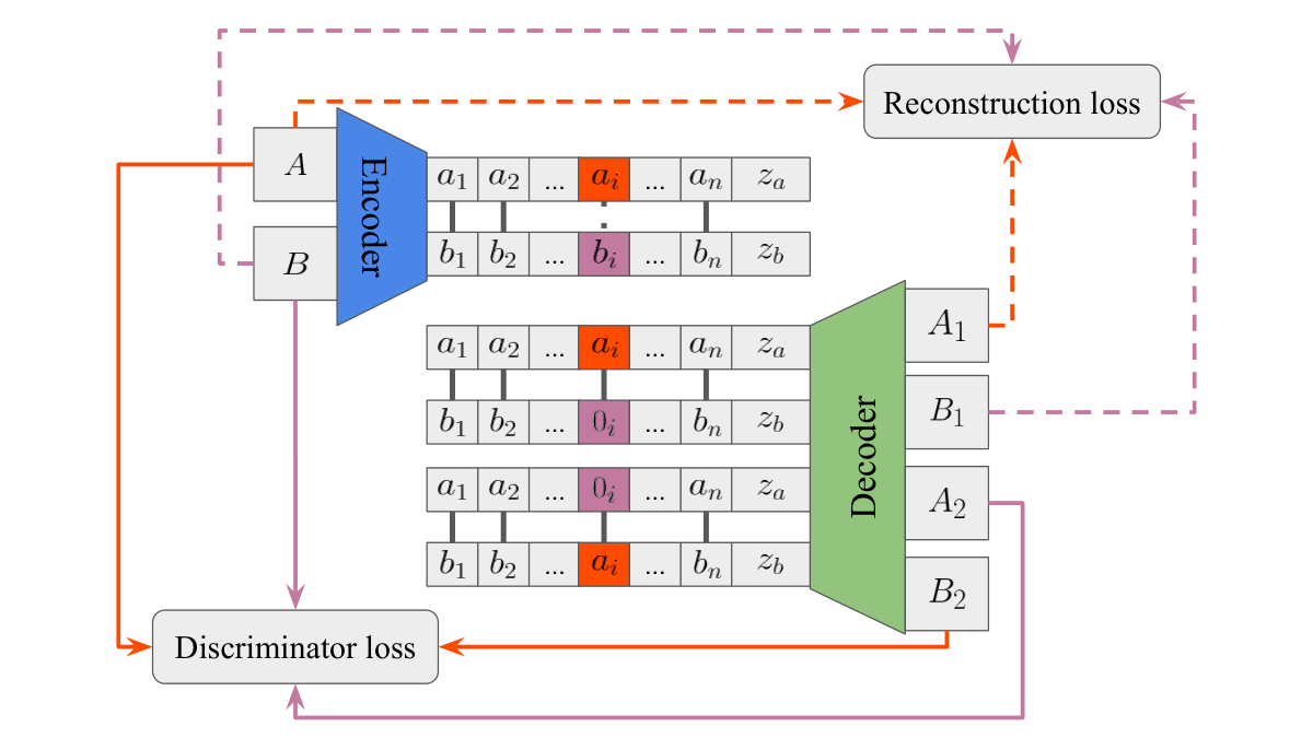
We focus on one attribute each time in our framework. Let’s say we are at the -th attribute. and are required to have different labels, i.e., and , respectively. Under this setting, is always for the dominant pattern, while is for the recessive pattern. We copy directly as the latent representation of , and annihilate in the copy of as the latent representation of . The annihilating operation means replacing all elements with zeros, and plays a key role in disentangling the attribute, which will be discussed in details in Section 3.3. By swapping and , we obtain two new latent representations and that are supposed to be decoded into and , respectively. Via a decoder , we can get four newly generated images , , and .
| (2) | ||||
Out of these four children, and are the direct reconstructions of and , respectively, while and are novel crossbreeds. The reconstruction losses between and , and , respectively, ensure the quality of directly reconstructed samples. Besides, using an adversarial discriminator that helps make generated samples indistinguishable from , and indistinguishable from , we can consider attribute-related information to be encoded in .
3.2 Loss Functions
Given two images and and their labels and which are different at the -th position, the data flow can be summarized by (1) and (2). We force the -th latent encoding of to be zero in order to prevent from trivial solutions as we will discuss in Section 3.3.
The encoder and decoder receive two types of losses: (1) the reconstruction loss,
| (3) |
which measures the reconstruction quality after a sequence of encoding and decoding; (2) the standard GAN loss,
| (4) |
which measures how realistic the generated images are. The discriminator takes the generated image and the -th element of its label as inputs, and outputs a number which indicates how realistic the input image is. The larger the number is, the more realistic the image is. Omitting the coefficient, the loss function for the encoder and decoder is
| (5) |
The discriminator receives the standard GAN discriminator loss
| (6) | ||||
| (7) | ||||
| (8) |
where drives to tell from , and drives to tell from .
3.3 Annihilating Operation Prevents from Trivial Solutions
Through the experiments, we can observe that there exist trivial solutions to our model without the annihilating operation. We just take the single-attribute case as an example. Suppose that and , we can get four children without annihilating operation
| (9) |
The reconstruction loss makes it invertible from the latent encodings to the image. The adversarial discriminator is supposed to disentangle the attribute from other information by telling whether looks as real as and looks as real as or not. As is well-known, a generative adversarial network obtains the best solution when achieving the Nash equilibrium. But without the annihilating operation, information of the whole image could be encoded intensively into the attribute-relevant part, which just means
| (10) |
In this way, we have the following four children:
| (11) |
In this situation, the discriminator cannot discriminate from , since they share the same latent encodings. By the reconstruction procedure, and lead to the same image, which is against our expectation that should depict the person from with the attribute borrowed from . The same situation appears in the case of and as well.
In order to get rid of these trivial solutions, we adopt the annihilating operation by replacing the recessive pattern with a zero tensor of the same size11 1 Use tf.zeros_like() in TensorFlow implementation., i.e., knocking it out, and keeping the other part alive. In fact, if information of the whole image were encoded only into the attribute-relevant part, the four children in this case would be
| (12) |
So, the encodings of and contain no information at all and therefore the person in the corresponding images of and , who is supposed to be the same as from , cannot be reconstructed at all, which is contradictory to our aim. Hence, the attribute-irrelevant part is necessary to encode certain information of images when implementing the annihilating operation.
3.4 Iterative Training
To reduce the difficulty of disentangling multiple attributes, we take the strategy of iterative training: we update our model using a pair of images with opposite labels at a certain position each time. Suppose that we are at the -th position, the label of image is , while the label of image is . During each iteration, as goes through from to repeatedly, our model fed with such a pair of images can disentangle multiple attributes one-by-one.
Compared with training with random pairs of images, iterative training is proved to be more effective. Random pairs of images means randomly selecting pairs of images each time without label constraints. A pair of images with different labels is called a useful pair.
We theoretically show that our iterative training mechanism is much more efficient than random image pairs especially when the dataset is unbalanced. All proofs can be found in the Appendix.
Theorem 1.
Let denote the whole multi-attribute image dataset, where is a multi-attribute image and its label is an -dimensional vector. There are totally kinds of labels, denoted by . The number of images with label is , and . To select all useful pairs at least once, the expected numbers of iterations needed for randomly selecting pairs and for iterative training are denoted by and respectively. Then,
| (13) | ||||
| (14) |
where represents the indices of labels where the -th element is , and represents the indices of labels where the -th element is .
Definition 1.
(Balancedness) Define the balancedness of a dataset described above with respect to the -th attribute as follows:
| (15) |
where represents the indices of labels where the -th element is , and represents the indices of labels where the -th element is .
Theorem 2.
We have , when
| (16) |
Specifically, holds true for all .
The property of the function suits well with the definition of balancedness, because it attains the same value for and , which is invariant to different labeling methods. Its value gets larger as the dataset becomes more unbalanced. The minimum is obtained at , which is the case of a balanced dataset.
Theorem 2 demonstrates that the iterative training mechanism is always more efficient than random pairs of images when the number of attributes met the criterion (16). As the dataset becomes more unbalanced, goes larger, which means (16) can be more easily satisfied. More importantly, iterative training helps stabilize the training process on unbalanced datasets. For example, given a two-attribute dataset, the number of data of each kind is as follows:
| Label | ||||
|---|---|---|---|---|
| Number of data |
If is a very large number, then it is highly likely that we will select a pair of images whose labels are and each time by randomly selecting pairs. We ignore the pair of images whose labels are and or and , though these two cases have equal probabilities of being chosen. Because they are not useful pairs, thus do not participated in training. In this case, most of the time the model is trained with respect to the second attribute, which will cause the final learnt model less effective to the first attribute. However, iterative training can prevent this from happening, since we update our model evenly with respect to two attributes.
4 Experimental Results
In this section, we perform different kinds of experiments on two real-world datasets to validate the effectiveness of our methods. We use the RMSProp (Sutskever et al., 2013) optimization method initialized by a learning rate of 5e-5 and momentum . All neural networks are equipped with Batch Normalization (Ioffe & Szegedy, 2015) after convolutions or deconvolutions. We used Leaky Relu (Maas et al., 2013) as the activation function in the encoder. Besides, we adopt strategies mentioned in Wasserstein GAN (Arjovsky et al., 2017) for stable training. We divide all images into training images and test images according to the ratio of 9:1. All of the following results are from test images without cherry-picking. More details can be found at https://github.com/Prinsphield/DNA-GAN.
4.1 Multi-PIE Database
![[Uncaptioned image]](1711.05415v2/extra/multipie/iter_110500_4.jpg)
![[Uncaptioned image]](1711.05415v2/extra/multipie/iter_111500_2.jpg)
![[Uncaptioned image]](1711.05415v2/extra/multipie/iter_114500_1.jpg)
![[Uncaptioned image]](1711.05415v2/extra/multipie/iter_118000_1.jpg)
![[Uncaptioned image]](1711.05415v2/extra/multipie/iter_118000_2.jpg)
![[Uncaptioned image]](1711.05415v2/extra/multipie/iter_120500_4.jpg)
The Multi-PIE (Gross et al., 2010) face database contains over 750,000 images of 337 subjects captured under 15 view points and 19 illumination conditions. We collecte all front faces images of different illuminations and align them based on 5-point landmarks on eyes, nose and mouth. All aligned images are resized into as inputs in our experiments. We label the light illumination face images by 1 and the dark illumination face images by 0. As shown in Figure 2, the illumination on one face is successfully transferred into the other face without modifying any other information in the images. This demonstrates that DNA-GAN can effectively disentangle the illumination factor from other factors in the latent space.
4.2 CelebA Dataset
CelebA (Liu et al., 2015) is a dataset composed of 202599 face images and 40 attribute binary vectors and 5 landmark locations. We use the aligned and cropped version and scaled all images down to . To better demonstrate the advantage of our method, we choose TD-GAN (Wang et al., 2017) and IcGAN (Perarnau et al., 2016) for comparisons.
As we mentioned before, TD-GAN requires the explicit id information in the label, thus cannot be applied to the CelebA dataset directly. To overcome this limitation, we use some channels to encode the id information in its latent representations. In our experiments, the id information is preserved when swapping the attribute information in the latent encodings. We also compared the experimental results of IcGAN with ours in the celebA dataset. The following results are obtained using the the official code and pre-trained celebA model provided by the author22 2 https://github.com/Guim3/IcGAN.


As displayed in Figure 3a, modified TD-GAN encounters the problem of trivial solutions. Without id information explicitly contained in the label, TD-GAN encodes the information of the whole image into the attribute-related part in the latent representations. As a result, two faces are swapped directly. Whereas in Figure 3b, the quality of images generated by IcGAN are very bad, which is probably due to the multi-stage training process of IcGAN. Since the overall effect of the model relies much on the each stage.
DNA-GAN is able to disentangle multiple attributes in the latent representations as shown in Figure 4. Since different attributes are encoded in different DNA pieces in our latent representations, we are able to interpolate the attribute subspaces by linear combination of disentangled encodings. Figure 4a, 4b and 4c present disentangled attribute subspaces spanned by any two attributes of Bangs, Eyeglasses and Smiling. They demonstrate that our model is effective in learning disentangled representations. Figure 4d shows the hairstyle transfer process among different Bangs styles. It is worth mentioning that the top-left image in Figure 4d is outside the CelebA dataset, which further validate the generalization potential of our model on unseen data. Please refer to Figure 5 in the Appendix for more results.


5 Conclusions
We have propose a supervised model called DNA-GAN that can learn disentangled representations from multi-attribute images. The latent representations of images are DNA-like, consisting of attribute-relevant and attribute-irrelevant parts. By the annihilating operation and attribute hybridization, we are able to create new latent representations which could be decoded into novel images with designed attributes. The iterative training strategy effectively overcomes the difficulty of training on unbalanced datasets and helps disentangle multiple attributes in the latent space. The experimental results not only demonstrate that DNA-GAN is effective in learning disentangled representations and image editing, but also point out its potential in interpretable deep learning, image understanding and transfer learning.
However, there still exist certain limitations of our model. Without strong guidance on the attribute-irrelevant parts, some background information may be encoded into the attribute-relevant part. As being shown in Figure 4, the background color gets changed when swapping attributes. Besides, our model may fail when several attributes are highly correlated with each other. For example, male and mustache are statistically dependent, which are hard to disentangle in the latent representations. These are left as our future work.
Acknowledgement
This work was supported by High-performance Computing Platform of Peking University and the National Science Foundation of China for grant U1604153.
References
- Arjovsky et al. (2017) Martín Arjovsky, Soumith Chintala, and Léon Bottou. Wasserstein GAN. CoRR, abs/1701.07875, 2017.
- Bengio et al. (2013) Yoshua Bengio, Aaron C. Courville, and Pascal Vincent. Representation learning: A review and new perspectives. IEEE Trans. Pattern Anal. Mach. Intell., 35(8):1798–1828, 2013.
- Bouchacourt et al. (2017) Diane Bouchacourt, Ryota Tomioka, and Sebastian Nowozin. Multi-level variational autoencoder: Learning disentangled representations from grouped observations. CoRR, abs/1705.08841, 2017.
- Chen et al. (2016) Xi Chen, Xi Chen, Yan Duan, Rein Houthooft, John Schulman, Ilya Sutskever, and Pieter Abbeel. Infogan: Interpretable representation learning by information maximizing generative adversarial nets. In Advances in Neural Information Processing Systems 29, pp. 2172–2180, 2016.
- Goodfellow et al. (2014) Ian J. Goodfellow, Jean Pouget-Abadie, Mehdi Mirza, Bing Xu, David Warde-Farley, Sherjil Ozair, Aaron C. Courville, and Yoshua Bengio. Generative adversarial nets. In Advances in Neural Information Processing Systems 27, pp. 2672–2680, 2014.
- Gross et al. (2010) Ralph Gross, Iain A. Matthews, Jeffrey F. Cohn, Takeo Kanade, and Simon Baker. Multi-pie. Image Vision Comput., 28(5):807–813, 2010.
- Higgins et al. (2016) Irina Higgins, Loic Matthey, Arka Pal, Christopher Burgess, Xavier Glorot, Matthew Botvinick, Shakir Mohamed, and Alexander Lerchner. beta-vae: Learning basic visual concepts with a constrained variational framework. 2016.
- Ioffe & Szegedy (2015) Sergey Ioffe and Christian Szegedy. Batch normalization: Accelerating deep network training by reducing internal covariate shift. In Proceedings of the 32nd International Conference on Machine Learning, ICML 2015, pp. 448–456, 2015.
- Isola et al. (2016) Phillip Isola, Jun-Yan Zhu, Tinghui Zhou, and Alexei A. Efros. Image-to-image translation with conditional adversarial networks. CoRR, abs/1611.07004, 2016.
- Kingma & Welling (2013) Diederik P. Kingma and Max Welling. Auto-encoding variational bayes. CoRR, abs/1312.6114, 2013.
- Kulkarni et al. (2015) Tejas D. Kulkarni, William F. Whitney, Pushmeet Kohli, and Joshua B. Tenenbaum. Deep convolutional inverse graphics network. In Advances in Neural Information Processing Systems 28, pp. 2539–2547, 2015.
- Liu et al. (2017) Ming-Yu Liu, Thomas Breuel, and Jan Kautz. Unsupervised image-to-image translation networks. CoRR, abs/1703.00848, 2017.
- Liu et al. (2015) Ziwei Liu, Ping Luo, Xiaogang Wang, and Xiaoou Tang. Deep learning face attributes in the wild. In 2015 IEEE International Conference on Computer Vision, ICCV 2015, pp. 3730–3738, 2015.
- Maas et al. (2013) Andrew L Maas, Awni Y Hannun, and Andrew Y Ng. Rectifier nonlinearities improve neural network acoustic models. In Proc. ICML, volume 30, 2013.
- Mirza & Osindero (2014) Mehdi Mirza and Simon Osindero. Conditional generative adversarial nets. CoRR, abs/1411.1784, 2014.
- Pearson (1901) Karl Pearson. Liii. on lines and planes of closest fit to systems of points in space. The London, Edinburgh, and Dublin Philosophical Magazine and Journal of Science, 2(11):559–572, 1901.
- Perarnau et al. (2016) Guim Perarnau, Joost van de Weijer, Bogdan Raducanu, and Jose M. Álvarez. Invertible conditional gans for image editing. CoRR, abs/1611.06355, 2016.
- Roweis & Saul (2000) Sam T Roweis and Lawrence K Saul. Nonlinear dimensionality reduction by locally linear embedding. science, 290(5500):2323–2326, 2000.
- Siddharth et al. (2016) N Siddharth, Brooks Paige, Alban Desmaison, Jan-Willem van de Meent, Frank Wood, Noah D Goodman, Pushmeet Kohli, and Philip HS Torr. Learning disentangled representations in deep generative models. 2016.
- Smolensky (1986) Paul Smolensky. Information processing in dynamical systems: Foundations of harmony theory. Technical report, COLORADO UNIV AT BOULDER DEPT OF COMPUTER SCIENCE, 1986.
- Sutskever et al. (2013) Ilya Sutskever, James Martens, George E. Dahl, and Geoffrey E. Hinton. On the importance of initialization and momentum in deep learning. In Proceedings of the 30th International Conference on Machine Learning, ICML 2013, pp. 1139–1147, 2013.
- Taigman et al. (2016) Yaniv Taigman, Adam Polyak, and Lior Wolf. Unsupervised cross-domain image generation. CoRR, abs/1611.02200, 2016.
- Wang et al. (2017) Chaoyue Wang, Chaohui Wang, Chang Xu, and Dacheng Tao. Tag disentangled generative adversarial network for object image re-rendering. In Proceedings of the Twenty-Sixth International Joint Conference on Artificial Intelligence, IJCAI 2017, pp. 2901–2907, 2017.
- Yu et al. (2009) Kai Yu, Tong Zhang, and Yihong Gong. Nonlinear learning using local coordinate coding. In Advances in Neural Information Processing Systems 22, pp. 2223–2231, 2009.
- Zhou et al. (2017) Shuchang Zhou, Taihong Xiao, Yi Yang, Dieqiao Feng, Qinyao He, and Weiran He. Genegan: Learning object transfiguration and attribute subspace from unpaired data. CoRR, abs/1705.04932, 2017.
- Zhu et al. (2017) Jun-Yan Zhu, Taesung Park, Phillip Isola, and Alexei A. Efros. Unpaired image-to-image translation using cycle-consistent adversarial networks. CoRR, abs/1703.10593, 2017.
Appendix
To prove Theorem 1, we need the following lemma.
Lemma 1.
A set has different elements, from which elements are being selected equally likely with replacement. The expected number of trials needed to collect a subset of elements is
Proof.
Let be the time to collect all elements in the subset , and let be the time to collect the -th new elements after elements in have been collected. Observe that the probability of collecting a new element is . Therefore, is a geometrically distributed random variable with expectation . By the linearity of expectations, we have:
∎
Proof.
(of Theorem 1)
We first consider the case of randomly selecting pairs. All possible image pairs are actually in the product space , whose cardinality is . If we take the order of two images in a pair into consideration, the number of possible pairs is . Recall that the useful pair denotes a pair of image of different labels. Therefore, the number of all useful pairs is . By Lemma 1, the expected number of iterations for randomly selecting pairs to select all useful pairs at least once is
| (17) |
Now we consider the case of iterative training. We always select a pair of images of different labels each time. Suppose we are selecting images with opposite labels at the -th position. Let denote the indices of all labels with the -th element , and denote the indices of all labels with the -th element , where . Then we consider the subproblem by neglecting the first position in data labels, the number of all possible pairs is (regarding of order), and the number of useful pairs is
| (18) |
Therefore, the expectation to select all useful pairs at least once regardless of the -th element in the label is
| (19) |
Since we rotate the subscript from to , the expected number of iterations for iterative training to select all useful pairs at least once is
| (20) |
∎
Proof.
(of Theorem 2) We firstly show that
| (21) |
According to the result of Theorem 1 and the Definition 1 of balancedness, we have
| (22) |
Specifically, if ,
| (23) |
The inequality holds true forever.
∎


