IKBT: solving closed-form Inverse Kinematics with Behavior Tree

As shown in Fig. 1, the system input takes symbolic Denavit––Hartenberg (DH) parameters and calculates symbolic forward kinematic equations in the form of a 4x4 homogeneous transformation. For a 6-DOF robot, the transformation matrix $T^{6}_{0}$ is computed as

By convention, each transformation matrix takes a coordinate from the subscript frame and transforms it to the superscript frame ($T^{6}_{0}$ transforms from frame 0 to frame 6).

We denote the desired robot end effector pose as $T_{d}$. Then the inverse kinematics problem can be stated as solving

(where $q_{i}$ are the unknown joint variables) for all sets of joint variables ($q_{i}=\theta_{i}$ or $d_{i}$) which satisfy 2. Related equations which can be used to find soluble equations include:

IKBT first symbolically calculates and simplifies these intermediate results (3 - 5) to augment (1). Each of these matrix equations creates 12 scalar equations (one for each element in the first three rows) which can be searched for solvable equations. After generating these matrices, each scalar equation is categorized by the number of unsolved joint variables, $q_{i}$, into three lists according to the number of unsolved variables in each equation (1, 2, and 3-or-more unknowns). As each variable is solved, this scan is repeated. The current toolbox examines equations containing 1- and 2-unsolved variables.

The Behavior Tree’s leaf nodes transform, or identify and solve, a particular kind of equation (See detail in the following section ”Transforms and Solvers”). For example, one pair of nodes identifies and solves scalar equations of one-unknown of the form $A=\sin(B\theta_{j}+C)$ or $A=\cos(B\theta_{j}+C)$ where $A,B,C$ are known expressions, and $\theta_{j}$ is unknown.

After all joint variables are solved, the solution graph and the solution vectors ($2^{n}$ joint vectors in symbolic form correctly associating the multiplicity of each variable) are constructed. A LaTeXreport, C++ and Python code, containing symbolic solutions for all possible poses, is also generated.

Behavior Trees have been explored in the context of humanoid robot control [6, 9, 10], collaborative robotics [11, 8], and as a modeling language for intelligent robotic surgical procedures [12, 13].

The work reported here is the first to our knowledge to use Behavior Trees to encode algorithms for reasoning about and solving mathematical equations symbolically. When implementing intelligent behavior with Behavior Trees, the designer of a robotic control system breaks the task down into modules (Behavior Tree leaves) which return either “success” or “failure” when called by parent nodes. Higher level nodes define composition rules to combine the leaves including: Sequence, Selector, and Parallel node types which also return “success” or “failure”. A Sequence node defines the order of execution of leaves and returns success if all leaves succeed in order. A Selector node (called “Priority” by some authors) tries leaf behaviors in a fixed order, returns success when a node succeeds, and returns failure if all leaves fail. We also implemented a “Parallel” node (represented as “OR” in Fig. 2), which executes all leaves regardless of their return status, and returns success if any one of the leaves succeeds. The IKBT structure used for our current results is shown in Fig.2.

Before solving, IKBT looks through 1- and 2- unknown equation lists, and applies sum-of-angle and substitution transformations which may reduce number of unknown variables. The “Assigner” node assigns the current variable to all solvers. For each joint variable, it tries out all solvers in the toolbox until it is solved (or we reach the maximum trial number). When a joint variable is solved, the solver marks it as solved, and reduces the number of unsolved variables by one, for all equations involved this variable. When multiple solvers can solve a joint variable, the solutions are compared using a “Ranker” node which selects preferred solution forms over others. For example, $\theta_{4}=$atan2($y,x$) is preferred over $\theta_{4}=\mathrm{arcsin}(y/r)$ because it has only one solution. IKBT repeats this until all variables are solved. Finally the solutions, report, code generation, and dependency graph are generated.

Transformation nodes make equations easier to solve by reducing the number of unknown variables.

1. 1.

   Sum of angle transform

   $$\sin(\theta_{x}\pm\theta_{y})\rightarrow\sin(\theta_{xy})$$

   $$\cos(\theta_{x}\pm\theta_{y})\rightarrow\cos(\theta_{xy})$$

   Although the sum-of-angle simplification is done by sympy’s simplify operation, creation of a new variable ($\theta_{xy}$) is done by this node.

2. 2.

   Substitution transform: looks for two equations such that one contains the other, and replaces the partial expression with a unknown value. For example, the following pair of equations:

   $$\sin(\theta_{x})+a\cdot\cos(\theta_{y})=b$$

   $$a\cdot\cos(\theta_{y})=c$$

   The first equation is transformed to:

   $$\sin(\theta_{x})+c=b$$

   Eliminating one unknowns so that $\theta_{x}$ can be solved.

The IKBT contains a set of solvers that identifies an expression that fits a rule set and return the respective solutions. These rules are used by human experts when solving inverse kinematics problems, and not are specific to any DOF or robot configuration.

1. 1.

   algebraic solver
   Identifies pattern

   $$a+b\theta=c$$

   where $b\neq 0$. Solves for

   $$\theta=\frac{c-a}{b}$$

   as well as

   $$a+bd_{x}=c$$

   giving

   $$d_{x}=\frac{c-a}{b}$$

2. 2.

   sine or cosine solver
   Identifies pattern

   $$\sin(\theta)=a,\quad\quad\cos(\theta)=b$$

   Solves for

   $$\theta=\arcsin(a),\quad\quad\theta=\arccos(b)$$

   or

   $$\theta=\pi-\arcsin(a),\quad\quad\theta=-\arccos(b)$$

3. 3.

   tangent solver
   identifies a pattern in two equations containing

   $$\sin(\theta)=aC_{1}\quad and\quad\cos(\theta)=bC_{2}$$

   If neither $C_{1}$ or $C_{2}$ contain unsolved variables:

   $$\theta=\atantwo(\frac{a}{C_{1}},\frac{b}{C_{2}})$$

   Sometimes $C_{1}$ and $C_{2}$ contain common unsolved variables, which can be canceled out by division. In this case we use a new coefficient $C$:

   $$C=\frac{C_{1}}{C_{2}}$$

   $$\theta=\atantwo(\frac{a}{C},b)\quad C>0$$

   $$\theta=\atantwo(-\frac{a}{C},-b)\quad C<0$$

   Terms which are solvable by tangent solver are often also solvable by sine or cosine solver. As shown in Fig 2, IKBT takes this into consideration by comparing the solutions from the above-mentioned solvers, and determines the optimal solution. This selection is done by the Ranking node.

4. 4.

   Sine and cosine solver

   Identifies

   $$a\cdot\sin(\theta)+b\cdot\cos(\theta)=0$$

   giving

   $$\theta=\atantwo(-b,a),\quad\quad\theta=\atantwo(-b,a)+\pi$$

   as well as

   $$a\cdot\sin(\theta)+b\cdot\cos(\theta)=c$$

   giving

   $$\theta=\atantwo(a,b)+\atantwo(\pm\sqrt{a^{2}+b^{2}-c^{2}},c)$$

5. 5.

   Simultaneous equation solver [3] Identifies two equations:

   $$a\sin(\theta)+b\cos(\theta)=c\qquad a\cos(\theta)-b\sin(\theta)=d$$

   Giving the solution:

   $$\theta=\atantwo(ac-bd,ad+bc)$$

6. 6.

   $x^{2}y^{2}$ solver

   Identifies two equations that contain $P_{x}$, $P_{y}$, and/or $P_{z}$, that can be squared and added together to cancel out unsolved variables (other than the intended variable), and get a new equation with pattern [14] :

   $$-\sin(\theta)P_{x}+\cos(\theta)P_{y}=d$$

   Giving solutions:

   $$\theta=\atantwo(P_{y},P_{x})-\atantwo(d,\pm\sqrt{{P_{x}}^{2}+{P_{y}}^{2}-d^{2}})$$

The solutions produced by inverse kinematics are typically interdependent in that results obtained early in the process are used to solve later results. For example, one may have

in which $\theta_{4}$ depends on $\cos(\theta_{45})=\cos(\theta_{4}+\theta_{5})$ as well as some constants. In principle, it is possible to substitute these dependencies until there are no joint variables on the right hand side, but this makes the solutions difficult to compare with previously published hand solutions. In the above example, there are two solutions to the $\operatorname{asin}()$ operator, and additional multiplicity could come from the solution method for $\theta_{45}$.

Thus the two sources of multiple solutions are: A) each joint variable may have multiple solutions due to its solver’s characteristic; and B) dependence of the solution on other solved joint variables. For example,

(where we have used the subscript $s$ to separate joint numbers from solution numbers. For example, $\theta_{1s2}$ means solution 2 of $\theta_{1}$). Now that $\theta_{1}$ is solved, we can write

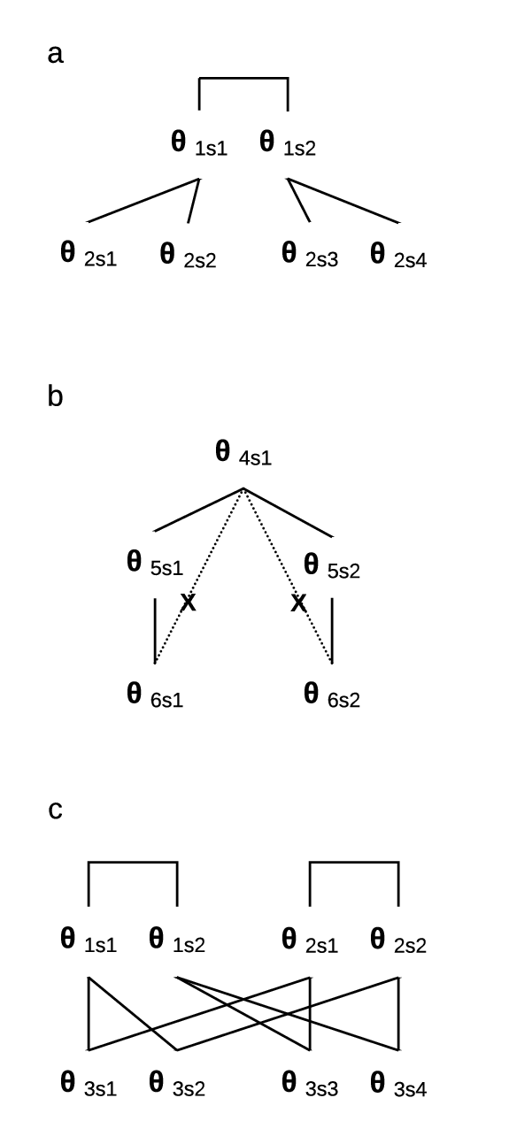
In the resulting graph (shown in Fig. 3 a), each joint solution (e.g. $\theta_{2s1}$, $\theta_{2s2}$, etc.) is a node. A parent node is the node that appears in another node’s solution expressions, in this example, $\theta_{1s1}$ is the parent of $\theta_{2s2}$ . A node and its parent/child node are connected with an edge.

When building a dependency graph, we implemented redundancy elimination to ensure the correct relations between joint variables. Redundancy is defined as a dependency that traced back to a higher level parent can be mediated by a lower level and direct parent. If a joint variable $\theta_{6}$ has the following solution:

And $\theta_{5}$ has solution:

Though the solution of $\theta_{6}$ involves both $\theta_{4}$ and $\theta_{5}$, its dependency to $\theta_{4}$ is redundant. Given that $\theta_{5}$ is also dependent on $\theta_{4}$, the effects of choosing different $\theta_{4}$ values (if applicable) on $\theta_{6}$ are conveyed through $\theta_{5}$. Therefore, when building a graph, only the edges between direct child-parents are added, in this case, Edge $(\theta_{6},\theta_{5})$ and Edge$(\theta_{5},\theta_{4})$. Shown in Fig. 3 b).

Classical search algorithms (breadth-first search and depth-first search) are used to traverse the graph and find correct ancestor nodes, where the current variable is the start point and the ancestors are the goals.

As required by many planning and control softwares, IKBT is capable of grouping variables into solution sets that have all possible joint configurations for the given end-effector configuration. To generate correct sets of solutions, the following steps are carried out to match the variables: First, all parents nodes are extracted from each solution expression, and formed subsets of variables. Secondly, the subsets are sorted by size of their content. Search starts from the largest subsets, and looks for the variables that are a part of the joint space, but not in the set, till all variables are found. A scoring system is applied on all subsets (other than the starting set) to focus the search on the more likely candidate first.

Using the Fig. 3 a) as an example, the solutions can be grouped into: [$\theta_{1s1}$, $\theta_{2s1}$], [$\theta_{1s1}$, $\theta_{2s2}$], [$\theta_{1s2}$, $\theta_{2s3}$], and [$\theta_{1s2}$, $\theta_{2s4}$].

The multiple dependencies can be linked by a common dependency further up, or they can be independent. Although traditionally this structure is represented as a tree, we discovered cases in which variables have multiple independent “parents” and thus a graph is required instead.

For example, $\theta_{1}$ and $\theta_{2}$ are independent to each other:

And $\theta_{3}$ depends on both $\theta_{1}$ and $\theta_{2}$:

The dependency graph is shown in Fig. 3 c).

One example robot solution in Results section shows the necessity of using graph representation.

To prove that the inverse kinematics solution equations from IKBT are correct, we conducted the following verification process, as shown in Fig. 4 . First, we constructed a valid numerical transformation matrix from a reachable pose. Then used numbers from the transformation matrix and the inverse kinematics solutions equations to get the numerical values for each pose. If the inverse kinematics solutions are correct, one of the poses should match the starting pose value. Next, compute the forward kinematics using each numerical pose. If the resulted transformation matrix is the same (within a stringent range) as the starting matrix, then we can safely draw the conclusion that this pose has correct inverse kinematics solution.

If a pose is not reachable by the robot (for example due to distance of a point extending beyond the length of the arm, but not considering joint limits), at least in generated code output, the solution must have a means to detect this case. In inverse kinematic solution equations, unreachable poses generate intermediate values outside the domain of transcendental functions, for example:

or would require complex joint angles:

Both the C++ and Python output modules of IKBT generate code which checks numerical arguments of inverse trig functions and square roots for such cases and returns a flag to indicate an unreachable pose.

We tested IKBT on many sets of DH parameters, representing serial arm robot designs (including commercial robots, and solved design examples from student homework), the successful solving rate is listed in Table I. As the DOF number increases, the problem becomes more complex and the success rate decreases. In general it solves most of the robots, up to 6 DOF. Note that IKBT can solve robots regardless of their configurations, e.g. IKBT does not require robots having three intersecting axes.

Source code can be found at: https://github.com/uw-biorobotics/IKBT. The DH parameters of all these robots are stored as part of the source code (in ik_robots.py), for purpose of testing and reproducing the results. Instructions are on the GitHub page.

Here PUMA560 is used as an example to illustrate how IKBT solves inverse kinematics problems. PUMA 560 was a commercial robot with six rotary joints and four joint offsets, well-known for its challenging inverse kinematics properties. The PUMA 560 has three axes intersecting at its wrist. The known variables are: $a_{2}$, $a_{3}$, $d_{3}$, and $d_{4}$.

First forward kinematics was calculated from DH parameters:

(where $T_{d}$ is the “desired position”, $T_{s}$ symbolic expressions, $T_{0}^{6}$ transformation matrix from frame 0 to 6)

$v_{1}=$

$v_{2}=$

where $c_{1}=cos(\theta_{1})$, $s_{23}=sin(\theta_{2}+\theta_{3})$ etc.

IKBT solved these variables in the following order:

1. 1.

   $\theta_{1}$, chosen solver: sinANDcos

   	$\displaystyle\theta_{1s1}=$	$\displaystyle\operatorname{atan2}{(Px,-Py)}+$
   		$\displaystyle\operatorname{atan2}{(\sqrt{Px^{2}+Py^{2}-d_{3}^{2}},-d_{3})}$
   	$\displaystyle\theta_{1s2}=$	$\displaystyle\operatorname{atan2}{(Px,-Py)}+$
   		$\displaystyle\operatorname{atan2}{(-\sqrt{Px^{2}+Py^{2}-d_{3}^{2}},-d_{3})}$

2. 2.

   $\theta_{3}$, chosen solver: $x^{2}y^{2}$

   	$\displaystyle\theta_{3s1}$	$\displaystyle=\operatorname{atan2}{(-2a_{2}d_{4},2a_{2}a_{3})}+$
   		$\displaystyle\operatorname{atan2}(\sqrt{s-(t+(Px\cos{(\theta_{1s1})}+Py\sin{(\theta_{1s1})})^{2})^{2}},$
   		$\displaystyle t+(Px\cos{(\theta_{1s1})}+Py\sin{(\theta_{1s1})})^{2})$
   	$\displaystyle\theta_{3s2}$	$\displaystyle=\operatorname{atan2}{(-2a_{2}d_{4},2a_{2}a_{3})}+$
   		$\displaystyle\operatorname{atan2}(-\sqrt{s-(t+(Px\cos{(\theta_{1s1})}+Py\sin{(\theta_{1s1})})^{2})^{2}},$
   		$\displaystyle t+(Px\cos{(\theta_{1s1})}+Py\sin{(\theta_{1s1})})^{2})$
   	$\displaystyle\theta_{3s3}$	$\displaystyle=\operatorname{atan2}{(-2a_{2}d_{4},2a_{2}a_{3})}+$
   		$\displaystyle\operatorname{atan2}(\sqrt{s-(t+(Px\cos{(\theta_{1s2})}+Py\sin{(\theta_{1s2})})^{2})^{2}},$
   		$\displaystyle t+(Px\cos{(\theta_{1s2})}+Py\sin{(\theta_{1s2})})^{2})$
   	$\displaystyle\theta_{3s4}$	$\displaystyle=\operatorname{atan2}{(-2a_{2}d_{4},2a_{2}a_{3})}+$
   		$\displaystyle\operatorname{atan2}(-\sqrt{s-(t+(Px\cos{(\theta_{1s2})}+Py\sin{(\theta_{1s2})})^{2})^{2}},$
   		$\displaystyle t+(Px\cos{(\theta_{1s2})}+Py\sin{(\theta_{1s2})})^{2})$

   where,

   	$\displaystyle s=$	$\displaystyle 4a_{2}^{2}a_{3}^{2}+4a_{2}^{2}d_{4}^{2}$
   	$\displaystyle t=$	$\displaystyle Pz^{2}-a_{2}^{2}-a_{3}^{2}-d_{4}^{2}$

3. 3.

   $\theta_{23}$, chosen solver: simultaneous equation

   	$\displaystyle\theta_{23s1}$	$\displaystyle=\operatorname{atan2}(Pz(-a_{2}\cos{(\theta_{3s3})}-a_{3})-$
   		$\displaystyle(-Px\cos{(\theta_{1s2})}-$
   		$\displaystyle Py\sin{(\theta_{1s2})})(a_{2}\sin{(\theta_{3s3})}-d_{4}),$
   		$\displaystyle Pz(a_{2}\sin{(\theta_{3s3})}-d_{4})+$
   		$\displaystyle(-Px\cos{(\theta_{1s2})}-Py\sin{(\theta_{1s2})})$
   		$\displaystyle(-a_{2}\cos{(\theta_{3s3})}-a_{3}))$
   	$\displaystyle\theta_{23s2}$	$\displaystyle=\operatorname{atan2}(Pz(-a_{2}\cos{(\theta_{3s2})}-a_{3})-$
   		$\displaystyle(-Px\cos{(\theta_{1s1})}-$
   		$\displaystyle Py\sin{(\theta_{1s1})})(a_{2}\sin{(\theta_{3s2})}-d_{4}),$
   		$\displaystyle Pz(a_{2}\sin{(\theta_{3s2})}-d_{4})+$
   		$\displaystyle(-Px\cos{(\theta_{1s1})}-Py\sin{(\theta_{1s1})})$
   		$\displaystyle(-a_{2}\cos{(\theta_{3s2})}-a_{3}))$
   	$\displaystyle\theta_{23s3}$	$\displaystyle=\operatorname{atan2}(Pz(-a_{2}\cos{(\theta_{3s1})}-a_{3})-$
   		$\displaystyle(-Px\cos{(\theta_{1s1})}-$
   		$\displaystyle Py\sin{(\theta_{1s1})})(a_{2}\sin{(\theta_{3s1})}-d_{4}),$
   		$\displaystyle Pz(a_{2}\sin{(\theta_{3s1})}-d_{4})+$
   		$\displaystyle(-Px\cos{(\theta_{1s1})}-Py\sin{(\theta_{1s1})})$
   		$\displaystyle(-a_{2}\cos{(\theta_{3s1})}-a_{3}))$
   	$\displaystyle\theta_{23s4}$	$\displaystyle=\operatorname{atan2}(Pz(-a_{2}\cos{(\theta_{3s4})}-a_{3})-$
   		$\displaystyle(-Px\cos{(\theta_{1s2})}-$
   		$\displaystyle Py\sin{(\theta_{1s2})})(a_{2}\sin{(\theta_{3s4})}-d_{4}),$
   		$\displaystyle Pz(a_{2}\sin{(\theta_{3s4})}-d_{4})+$
   		$\displaystyle(-Px\cos{(\theta_{1s2})}-Py\sin{(\theta_{1s2})})$
   		$\displaystyle(-a_{2}\cos{(\theta_{3s4})}-a_{3}))$

4. 4.

   $\theta_{2}$, chosen solver: algebraic solver

   	$\displaystyle\theta_{2s1}$	$\displaystyle=\theta_{23s2}-\theta_{3s2}$
   	$\displaystyle\theta_{2s2}$	$\displaystyle=\theta_{23s4}-\theta_{3s4}$
   	$\displaystyle\theta_{2s3}$	$\displaystyle=\theta_{23s1}-\theta_{3s3}$
   	$\displaystyle\theta_{2s4}$	$\displaystyle=\theta_{23s3}-\theta_{3s1}$

5. 5.

   $\theta_{4}$, chosen solver: tangent

   	$\displaystyle\theta_{4s1}$	$\displaystyle=\operatorname{atan2}(r_{13}\sin{(\theta_{1s1})}-r_{23}\cos{(\theta_{1s1})},$
   		$\displaystyle r_{13}\cos{(\theta_{1s1})}\cos{(\theta_{23s2})}+$
   		$\displaystyle r_{23}\sin{(\theta_{1s1})}\cos{(\theta_{23s2})}-r_{33}\sin{(\theta_{23s2})})$
   	$\displaystyle\theta_{4s2}$	$\displaystyle=\operatorname{atan2}(-r_{13}\sin{(\theta_{1s1})}+r_{23}\cos{(\theta_{1s1})},$
   		$\displaystyle-r_{13}\cos{(\theta_{1s1})}\cos{(\theta_{23s2})}-$
   		$\displaystyle r_{23}\sin{(\theta_{1s1})}\cos{(\theta_{23s2})}+r_{33}\sin{(\theta_{23s2}))}$
   	$\displaystyle\theta_{4s3}$	$\displaystyle=\operatorname{atan2}(r_{13}\sin{(\theta_{1s2})}-r_{23}\cos{(\theta_{1s2})},$
   		$\displaystyle r_{13}\cos{(\theta_{1s2})}\cos{(\theta_{23s4})}+$
   		$\displaystyle r_{23}\sin{(\theta_{1s2})}\cos{(\theta_{23s4})}-r_{33}\sin{(\theta_{23s4})})$
   	$\displaystyle\theta_{4s4}$	$\displaystyle=\operatorname{atan2}(-r_{13}\sin{(\theta_{1s2})}+r_{23}\cos{(\theta_{1s2})},$
   		$\displaystyle-r_{13}\cos{(\theta_{1s2})}\cos{(\theta_{23s4})}-$
   		$\displaystyle r_{23}\sin{(\theta_{1s2})}\cos{(\theta_{23s4})}+r_{33}\sin{(\theta_{23s4})})$
   	$\displaystyle\theta_{4s5}$	$\displaystyle=\operatorname{atan2}(r_{13}\sin{(\theta_{1s2})}-r_{23}\cos{(\theta_{1s2})},$
   		$\displaystyle r_{13}\cos{(\theta_{1s2})}\cos{(\theta_{23s1})}+$
   		$\displaystyle r_{23}\sin{(\theta_{1s2})}\cos{(\theta_{23s1})}-r_{33}\sin{(\theta_{23s1})})$
   	$\displaystyle\theta_{4s6}$	$\displaystyle=\operatorname{atan2}(-r_{13}\sin{(\theta_{1s2})}+r_{23}\cos{(\theta_{1s2})},$
   		$\displaystyle-r_{13}\cos{(\theta_{1s2})}\cos{(\theta_{23s1})}-$
   		$\displaystyle r_{23}\sin{(\theta_{1s2})}\cos{(\theta_{23s1})}+r_{33}\sin{(\theta_{23s1})})$
   	$\displaystyle\theta_{4s7}$	$\displaystyle=\operatorname{atan2}(r_{13}\sin{(\theta_{1s1})}-r_{23}\cos{(\theta_{1s1})},$
   		$\displaystyle r_{13}\cos{(\theta_{1s1})}\cos{(\theta_{23s3})}+$
   		$\displaystyle r_{23}\sin{(\theta_{1s1})}\cos{(\theta_{23s3})}-r_{33}\sin{(\theta_{23s3})})$
   	$\displaystyle\theta_{4s8}$	$\displaystyle=\operatorname{atan2}(-r_{13}\sin{(\theta_{1s1})}+r_{23}\cos{(\theta_{1s1})},$
   		$\displaystyle-r_{13}\cos{(\theta_{1s1})}\cos{(\theta_{23s3})}-$
   		$\displaystyle r_{23}\sin{(\theta_{1s1})}\cos{(\theta_{23s3})}+r_{33}\sin{(\theta_{23s3})})$

6. 6.

   $\theta_{5}$, chosen solver: tangent

   	$\displaystyle\theta_{5s1}$	$\displaystyle=\operatorname{atan2}(\frac{1}{\sin{(\theta_{4s3})}}(-r_{13}\sin{(\theta_{1s2})}+$
   		$\displaystyle r_{23}\cos{(\theta_{1s2})}),-r_{13}\sin{(\theta_{23s4})}\cos{(\theta_{1s2})}-$
   		$\displaystyle r_{23}\sin{(\theta_{1s2})}\sin{(\theta_{23s4})}-r_{33}\cos{(\theta_{23s4})}$
   	$\displaystyle\theta_{5s2}$	$\displaystyle=\operatorname{atan2}(\frac{1}{\sin{(\theta_{4s7})}}(-r_{13}\sin{(\theta_{1s1})}+$
   		$\displaystyle r_{23}\cos{(\theta_{1s1})}),-r_{13}\sin{(\theta_{23s3})}\cos{(\theta_{1s1})}-$
   		$\displaystyle r_{23}\sin{(\theta_{1s1})}\sin{(\theta_{23s3})}-r_{33}\cos{(\theta_{23s3})})$
   	$\displaystyle\theta_{5s3}$	$\displaystyle=\operatorname{atan2}(\frac{1}{\sin{(\theta_{4s2})}}(-r_{13}\sin{(\theta_{1s1})}+$
   		$\displaystyle r_{23}\cos{(\theta_{1s1})}),-r_{13}\sin{(\theta_{23s2})}\cos{(\theta_{1s1})}-$
   		$\displaystyle r_{23}\sin{(\theta_{1s1})}\sin{(\theta_{23s2})}-r_{33}\cos{(\theta_{23s2})})$
   	$\displaystyle\theta_{5s4}$	$\displaystyle=\operatorname{atan2}(\frac{1}{\sin{(\theta_{4s6})}}(-r_{13}\sin{(\theta_{1s2})}+$
   		$\displaystyle r_{23}\cos{(\theta_{1s2})}),-r_{13}\sin{(\theta_{23s1})}\cos{(\theta_{1s2})}-$
   		$\displaystyle r_{23}\sin{(\theta_{1s2})}\sin{(\theta_{23s1})}-r_{33}\cos{(\theta_{23s1})})$
   	$\displaystyle\theta_{5s5}$	$\displaystyle=\operatorname{atan2}(\frac{1}{\sin{(\theta_{4s4})}}(-r_{13}\sin{(\theta_{1s2})}+$
   		$\displaystyle r_{23}\cos{(\theta_{1s2})}),-r_{13}\sin{(\theta_{23s4})}\cos{(\theta_{1s2})}-$
   		$\displaystyle r_{23}\sin{(\theta_{1s2})}\sin{(\theta_{23s4})}-r_{33}\cos{(\theta_{23s4})})$

   	$\displaystyle\theta_{5s6}$	$\displaystyle=\operatorname{atan2}(\frac{1}{\sin{(\theta_{4s1})}}(-r_{13}\sin{(\theta_{1s1})}+$
   		$\displaystyle r_{23}\cos{(\theta_{1s1})}),-r_{13}\sin{(\theta_{23s2})}\cos{(\theta_{1s1})}-$
   		$\displaystyle r_{23}\sin{(\theta_{1s1})}\sin{(\theta_{23s2})}-r_{33}\cos{(\theta_{23s2})})$
   	$\displaystyle\theta_{5s7}$	$\displaystyle=\operatorname{atan2}(\frac{1}{\sin{(\theta_{4s8})}}(-r_{13}\sin{(\theta_{1s1})}+$
   		$\displaystyle r_{23}\cos{(\theta_{1s1})}),-r_{13}\sin{(\theta_{23s3})}\cos{(\theta_{1s1})}-$
   		$\displaystyle r_{23}\sin{(\theta_{1s1})}\sin{(\theta_{23s3})}-r_{33}\cos{(\theta_{23s3})})$
   	$\displaystyle\theta_{5s8}$	$\displaystyle=\operatorname{atan2}(\frac{1}{\sin{(\theta_{4s5})}}(-r_{13}\sin{(\theta_{1s2})}+$
   		$\displaystyle r_{23}\cos{(\theta_{1s2})}),-r_{13}\sin{(\theta_{23s1})}\cos{(\theta_{1s2})}-$
   		$\displaystyle r_{23}\sin{(\theta_{1s2})}\sin{(\theta_{23s1})}-r_{33}\cos{(\theta_{23s1})})$

7. 7.

   $\theta_{6}$, chosen solver: tangent

   	$\displaystyle\theta_{6s1}$	$\displaystyle=\operatorname{atan2}(-\frac{1}{\sin{(\theta_{5s4})}}(-r_{12}\sin{(\theta_{23s1})}\cos{(\theta_{1s2})}-$
   		$\displaystyle r_{22}\sin{(\theta_{1s2})}\sin{(\theta_{23s1})}-r_{32}\cos{(\theta_{23s1})}),$
   		$\displaystyle\frac{1}{\sin{(\theta_{5s4})}}(-r_{11}\sin{(\theta_{23s1})}\cos{(\theta_{1s2})}-$
   		$\displaystyle r_{21}\sin{(\theta_{1s2})}\sin{(\theta_{23s1})}-r_{31}\cos{(\theta_{23s1})}))$
   	$\displaystyle\theta_{6s2}$	$\displaystyle=\operatorname{atan2}(-\frac{1}{\sin{(\theta_{5s8})}}(-r_{12}\sin{(\theta_{23s1})}\cos{(\theta_{1s2})}-$
   		$\displaystyle r_{22}\sin{(\theta_{1s2})}\sin{(\theta_{23s1})}-r_{32}\cos{(\theta_{23s1})}),$
   		$\displaystyle\frac{1}{\sin{(\theta_{5s8})}}(-r_{11}\sin{(\theta_{23s1})}\cos{(\theta_{1s2})}-$
   		$\displaystyle r_{21}\sin{(\theta_{1s2})}\sin{(\theta_{23s1})}-r_{31}\cos{(\theta_{23s1})}))$
   	$\displaystyle\theta_{6s3}$	$\displaystyle=\operatorname{atan2}(-\frac{1}{\sin{(\theta_{5s1})}}(-r_{12}\sin{(\theta_{23s4})}\cos{(\theta_{1s2})}-$
   		$\displaystyle r_{22}\sin{(\theta_{1s2})}\sin{(\theta_{23s4})}-r_{32}\cos{(\theta_{23s4})}),$
   		$\displaystyle\frac{1}{\sin{(\theta_{5s1})}}(-r_{11}\sin{(\theta_{23s4})}\cos{(\theta_{1s2})}-$
   		$\displaystyle r_{21}\sin{(\theta_{1s2})}\sin{(\theta_{23s4})}-r_{31}\cos{(\theta_{23s4})}))$
   	$\displaystyle\theta_{6s4}$	$\displaystyle=\operatorname{atan2}(-\frac{1}{\sin{(\theta_{5s2})}}(-r_{12}\sin{(\theta_{23s3})}\cos{(\theta_{1s1})}-$
   		$\displaystyle r_{22}\sin{(\theta_{1s1})}\sin{(\theta_{23s3})}-r_{32}\cos{(\theta_{23s3})}),$
   		$\displaystyle\frac{1}{\sin{(\theta_{5s2})}}(-r_{11}\sin{(\theta_{23s3})}\cos{(\theta_{1s1})}-$
   		$\displaystyle r_{21}\sin{(\theta_{1s1})}\sin{(\theta_{23s3})}-r_{31}\cos{(\theta_{23s3})}))$
   	$\displaystyle\theta_{6s5}$	$\displaystyle=\operatorname{atan2}(-\frac{1}{\sin{(\theta_{5s6})}}(-r_{12}\sin{(\theta_{23s2})}\cos{(\theta_{1s1})}-$
   		$\displaystyle r_{22}\sin{(\theta_{1s1})}\sin{(\theta_{23s2})}-r_{32}\cos{(\theta_{23s2})}),$
   		$\displaystyle\frac{1}{\sin{(\theta_{5s6})}}(-r_{11}\sin{(\theta_{23s2})}\cos{(\theta_{1s1})}-$
   		$\displaystyle r_{21}\sin{(\theta_{1s1})}\sin{(\theta_{23s2})}-r_{31}\cos{(\theta_{23s2})}))$

   	$\displaystyle\theta_{6s6}$	$\displaystyle=\operatorname{atan2}(-\frac{1}{\sin{(\theta_{5s3})}}(-r_{12}\sin{(\theta_{23s2})}\cos{(\theta_{1s1})}-$
   		$\displaystyle r_{22}\sin{(\theta_{1s1})}\sin{(\theta_{23s2})}-r_{32}\cos{(\theta_{23s2})}),$
   		$\displaystyle\frac{1}{\sin{(\theta_{5s3})}}(-r_{11}\sin{(\theta_{23s2})}\cos{(\theta_{1s1})}-$
   		$\displaystyle r_{21}\sin{(\theta_{1s1})}\sin{(\theta_{23s2})}-r_{31}\cos{(\theta_{23s2})}))$
   	$\displaystyle\theta_{6s7}$	$\displaystyle=\operatorname{atan2}(-\frac{1}{\sin{(\theta_{5s7})}}(-r_{12}\sin{(\theta_{23s3})}\cos{(\theta_{1s1})}-$
   		$\displaystyle r_{22}\sin{(\theta_{1s1})}\sin{(\theta_{23s3})}-r_{32}\cos{(\theta_{23s3})}),$
   		$\displaystyle\frac{1}{\sin{(\theta_{5s7})}}(-r_{11}\sin{(\theta_{23s3})}\cos{(\theta_{1s1})}-$
   		$\displaystyle r_{21}\sin{(\theta_{1s1})}\sin{(\theta_{23s3})}-r_{31}\cos{(\theta_{23s3})}))$
   	$\displaystyle\theta_{6s8}$	$\displaystyle=\operatorname{atan2}(-\frac{1}{\sin{(\theta_{5s5})}}(-r_{12}\sin{(\theta_{23s4})}\cos{(\theta_{1s2})}-$
   		$\displaystyle r_{22}\sin{(\theta_{1s2})}\sin{(\theta_{23s4})}-r_{32}\cos{(\theta_{23s4})}),$
   		$\displaystyle\frac{1}{\sin{(\theta_{5s5})}}(-r_{11}\sin{(\theta_{23s4})}\cos{(\theta_{1s2})}-$
   		$\displaystyle r_{21}\sin{(\theta_{1s2})}\sin{(\theta_{23s4})}-r_{31}\cos{(\theta_{23s4})}))$