跳到论文正文
W Papers独立论文阅读器 arXiv:1711.05060 论文正文 计算阅读时间 · 0%
引用这篇论文根据当前论文元数据生成,正式投稿前建议核对。


License: arXiv.org perpetual non-exclusive license
arXiv:1711.05060v2 [cs.LG] 10 Dec 2018

∎

Dynamic Principal Projection for Cost-Sensitive Online Multi-Label Classification

Hong-Min Chu    Kuan-Hao Huang    Hsuan-Tien Lin Affiliation: CSIE Department, National Taiwan University, Taiwan E-mail: {r04922031, r03922062, htlin}@csie.ntu.edu.tw
Received: date / Accepted: date
Abstract

We study multi-label classification (MLC) with three important real-world issues: online updating, label space dimension reduction (LSDR), and cost-sensitivity. Current MLC algorithms have not been designed to address these three issues simultaneously. In this paper, we propose a novel algorithm, cost-sensitive dynamic principal projection (CS-DPP) that resolves all three issues. The foundation of CS-DPP is an online LSDR framework derived from a leading LSDR algorithm. In particular, CS-DPP is equipped with an efficient online dimension reducer motivated by matrix stochastic gradient, and establishes its theoretical backbone when coupled with a carefully-designed online regression learner. In addition, CS-DPP embeds the cost information into label weights to achieve cost-sensitivity along with theoretical guarantees. Experimental results verify that CS-DPP achieves better practical performance than current MLC algorithms across different evaluation criteria, and demonstrate the importance of resolving the three issues simultaneously.

Keywords: 
Multi-label classification Cost-sensitive Label space dimension reduction

1 Introduction

The multi-label classification (MLC) problem allows each instance to be associated with a set of labels and reflects the nature of a wide spectrum of real-world applications [8, 4, 12]. Traditional MLC algorithms mainly tackle the batch MLC problem, where the input data are presented in a batch [24, 28]. Nevertheless, in many MLC applications such as e-mail categorization [22], multi-label examples arrive as a stream. Online analysis is therefore required as batch MLC algorithms may not meet the needs to make a prediction and update the predictor on the fly. The needs of such applications can be formalized as the online MLC (OMLC) problem.

The OMLC problem is generally more challenging than the batch one, and many mature algorithms for the batch problem have not yet been carefully extended to OMLC. Label space dimension reduction (LSDR) is a family of mature algorithms for the batch MLC problem [7, 13, 17, 26, 14, 25, 33, 6, 2, 5]. By viewing the label set of each instance as a high-dimensional label vector in a label space, LSDR encodes each label vector as a code vector in a lower-dimensional code space, and learns a predictor within the code space. An unseen instance is predicted by coupling the predictor with a decoder from the code space to the label space. For example, compressed sensing (CS) [13] encodes using random projections, and decodes with sparse vector reconstruction; principal label space transformation (PLST) [26] encodes by projecting to the key eigenvectors of the known label vectors obtained from principal component analysis (PCA), and decodes by reconstruction with the same eigenvectors. This low-dimensional encoding allows LSDR algorithms to exploit the key joint information between labels to be more robust to noise and be more effective on learning [26]. Nevertheless, to the best of our knowledge, all the LSDR algorithms mentioned above are designed only for the batch MLC problem.

Another family of MLC algorithms that have not been carefully extended for OMLC contains the cost-sensitive MLC algorithms. In particular, different MLC applications usually come with different evaluation criteria (costs) that reflect their realistic needs. It is important to design MLC algorithms that are cost-sensitive to systematically cope with different costs, because an MLC algorithm that targets one specific cost may not always perform well under other costs [15]. Two representative cost-sensitive MLC algorithms are probabilistic classifier chain (PCC) [10] and condensed filter tree (CFT) [15]. PCC estimates the conditional probability with the classifier chain (CC) method [24] and makes Bayes-optimal predictions with respect to the given cost; CFT decomposes the cost into instance weights when training the classifiers in CC. Both algorithms, again, targets the batch MLC problem rather than the OMLC one.

From the discussions above, there is currently no algorithm that considers the three realistic needs of online updating, label space dimension reduction, and cost-sensitivity at the same time. The goal of this work is to study such algorithms. We first formalize the OMLC and cost-sensitive OMLC (CSOMLC) problems in Section 2 and discuss related work. We then extend LSDR for the OMLC problem and propose a novel online LSDR algorithm, dynamic principal projection (DPP), by connecting PLST with online PCA. In particular, we derive the DPP algorithm in Section 3 along with its theoretical guarantees, and resolve the issue of possible basis drifting caused by online PCA.

In Section 4, we further generalize DPP to cost-sensitive DPP (CS-DPP) to fully match the needs of CSOMLC with a theoretically-backed label-weighting scheme inspired by CFT. Extensive empirical studies demonstrate the strength of CS-DPP in addressing the three realistic needs in Section 5. In particular, we justify the necessity to consider LSDR, basis drifting and cost-sensitivity. The results show that CS-DPP significantly outperforms other OMLC competitors across different CSOMLC problems, which validates the robustness and effectiveness of CS-DPP, as concluded in Section 6.

2 Preliminaries and Related Work

For the MLC problem, we denote the feature vector of an instance as 𝐱∈ℝd\mathbf{x}\in\mathbb{R}^{d} and its corresponding label vector as 𝐲∈𝒴≡{+1,−1}K\mathbf{y}\in\mathcal{Y}\equiv\{+1,-1\}^{K}, where 𝐲⁡[k]=+1\mathbf{y}[k]=+1 iff the instance is associated with the kk-th label out of a total of KK possible labels. We let 𝐲⁡[k]∈{+1,−1}\mathbf{y}[k]\in\{+1,-1\} to conform with the common setting of online binary classification [9], which is equivalent to another scheme, 𝐲⁡[k]∈{1,0}\mathbf{y}[k]\in\{1,0\}, used in other MLC works [15, 24].

Traditional MLC methods consider the batch setting, where a training dataset 𝒟={(𝐱n,𝐲n)}n=1N\mathcal{D}=\{(\mathbf{x}_{n},\mathbf{y}_{n})\}_{n=1}^{N} is given at once, and the objective is to learn a classifier g:ℝd→{+1,−1}Kg\colon\mathbb{R}^{d}\rightarrow\{+1,-1\}^{K} from 𝒟\mathcal{D} with the hope that 𝐲^=g⁡(𝐱)\hat{\mathbf{y}}=g(\mathbf{x}) accurately predicts the ground truth 𝐲\mathbf{y} with respect to an unseen 𝐱\mathbf{x}. In this work, we focus on the OMLC setting, which assumes that instance (𝐱t,𝐲t)(\mathbf{x}_{t},\mathbf{y}_{t}) arrives in sequence from a data stream. Whenever an 𝐱t\mathbf{x}_{t} arrives at iteration tt, the OMLC algorithm is required to make a prediction 𝐲^t=gt​(𝐱t)\hat{\mathbf{y}}_{t}=g_{t}(\mathbf{x}_{t}) based on the current classifier gtg_{t} and feature vector 𝐱t\mathbf{x}_{t}. The ground truth 𝐲t\mathbf{y}_{t} with respect to 𝐱t\mathbf{x}_{t} is then revealed, and the penalty of 𝐲^t\hat{\mathbf{y}}_{t} is evaluated against 𝐲t\mathbf{y}_{t}.

Many evaluation criteria for comparing 𝐲\mathbf{y} and 𝐲^\hat{\mathbf{y}} have been considered in the literature to satisfy different application needs. A simple criterion [28] is the Hamming loss cham​(𝐲,𝐲^)c_{\textsc{ham}}(\mathbf{y},\hat{\mathbf{y}}) = 1K∑k=1K⟦𝐲[k]≠𝐲^[k]⟧\frac{1}{K}\sum^{K}_{k=1}\llbracket\mathbf{y}[k]\neq\hat{\mathbf{y}}[k]\rrbracket. The Hamming loss separately considers each label during evaluation. There are other criteria that jointly evaluate all labels, such as the F1 loss  [28]

cf​(𝐲,𝐲^)=1−2​∑k=1K⟦𝐲[k]=+1 and 𝐲^[k]=+1⟧∑k=1K(⟦𝐲[k]=+1⟧+⟦𝐲^[k]=+1⟧).c_{\textsc{f}}(\mathbf{y},\hat{\mathbf{y}})=1-2\dfrac{\sum\nolimits_{k=1}^{K}\llbracket\mathbf{y}[k]\!=\!+1\mbox{ and }\hat{\mathbf{y}}[k]\!=\!+1\rrbracket}{\sum\nolimits_{k=1}^{K}\left(\llbracket\mathbf{y}[k]\!=\!+1\rrbracket+\llbracket\hat{\mathbf{y}}[k]\!=\!+1\rrbracket\right)}.

In this work, we follow existing cost-sensitive MLC approaches [15] to extend OMLC to the cost-sensitive OMLC (CSOMLC) setting, which further takes the evaluation criterion as an additional input to the learning algorithm. We call the criterion a cost function and overload c:{+1,−1}K×{+1,−1}K→ℝc\colon\{+1,-1\}^{K}\times\{+1,-1\}^{K}\rightarrow\mathbb{R} as its notation. The cost function evaluates the penalty of 𝐲^\hat{\mathbf{y}} against 𝐲\mathbf{y} by c⁡(𝐲,𝐲^)c(\mathbf{y},\hat{\mathbf{y}}).We naturally assume that c⁡(⋅,⋅)c(\cdot,\cdot) satisfies c⁡(𝐲,𝐲)=0c(\mathbf{y},\mathbf{y})=0 and max𝐲^⁡c⁡(𝐲,𝐲^)≤1\max_{\hat{\mathbf{y}}}c(\mathbf{y},\hat{\mathbf{y}})\leq 1. The objective of a CSOMLC algorithm is to adaptively learn a classifier gt:ℝd→{+1,−1}Kg_{t}\colon\mathbb{R}^{d}\rightarrow\{+1,-1\}^{K} based on not only the data stream but also the input cost function cc such that the cumulative cost ∑t=1Tc⁡(𝐲t,𝐲^t)\sum_{t=1}^{T}c(\mathbf{y}_{t},\hat{\mathbf{y}}_{t}) with respect to the input cc, where 𝐲^t=gt​(𝐱t)\hat{\mathbf{y}}_{t}=g_{t}(\mathbf{x}_{t}), can be minimized.

Note that the cost function within the CSOMLC setting above corresponds to the example-based evaluation criteria for MLC, named because the prediction 𝐲^t\hat{\mathbf{y}}_{t} of each example is evaluated against the ground truth 𝐲t\mathbf{y}_{t} independently. More sophisticated evaluation criteria such as micro-based and macro-based criteria [27, 20] can also be found in the literature. The following equations highlight the difference between example-F1 (what our CSOMLC setting can handle), micro-F1 and macro-F1 when calculated on TT predictions

example-F1 loss =\displaystyle= 1−2T​∑t=1T∑k=1K⟦𝐲t[k]=+1 and 𝐲^t[k]=+1⟧∑k=1K(⟦𝐲t[k]=+1⟧+⟦𝐲^t[k]=+1⟧);\displaystyle 1-\frac{2}{T}\sum_{t=1}^{T}\frac{\sum\nolimits_{k=1}^{K}\llbracket\mathbf{y}_{t}[k]\!=\!+1\mbox{ and }\hat{\mathbf{y}}_{t}[k]\!=\!+1\rrbracket}{\sum\nolimits_{k=1}^{K}\left(\llbracket\mathbf{y}_{t}[k]\!=\!+1\rrbracket+\llbracket\hat{\mathbf{y}}_{t}[k]\!=\!+1\rrbracket\right)}\;\;\;{\color[rgb]{0,0,0};}
micro-F1 loss =\displaystyle= 1−2K​∑k=1K∑t=1T⟦𝐲t[k]=+1 and 𝐲^t[k]=+1⟧∑t=1T(⟦𝐲t[k]=+1⟧+⟦𝐲^t[k]=+1⟧);\displaystyle 1-\frac{2}{K}\sum_{k=1}^{K}\frac{\sum\nolimits_{t=1}^{T}\llbracket\mathbf{y}_{t}[k]\!=\!+1\mbox{ and }\hat{\mathbf{y}}_{t}[k]\!=\!+1\rrbracket}{\sum\nolimits_{t=1}^{T}\left(\llbracket\mathbf{y}_{t}[k]\!=\!+1\rrbracket+\llbracket\hat{\mathbf{y}}_{t}[k]\!=\!+1\rrbracket\right)}\;\;\;{\color[rgb]{0,0,0};}
macro-F1 loss =\displaystyle= 1−2​∑t=1T∑k=1K⟦𝐲t[k]=+1 and 𝐲^t[k]=+1⟧∑t=1T∑k=1K(⟦𝐲t[k]=+1⟧+⟦𝐲^t[k]=+1⟧).\displaystyle 1-2\frac{\sum\nolimits_{t=1}^{T}\sum_{k=1}^{K}\llbracket\mathbf{y}_{t}[k]\!=\!+1\mbox{ and }\hat{\mathbf{y}}_{t}[k]\!=\!+1\rrbracket}{\sum\nolimits_{t=1}^{T}\sum_{k=1}^{K}\left(\llbracket\mathbf{y}_{t}[k]\!=\!+1\rrbracket+\llbracket\hat{\mathbf{y}}_{t}[k]\!=\!+1\rrbracket\right)}\;\;\;{\color[rgb]{0,0,0}.}

In particular, the three criteria differ by the averaging process. Average example-F1 computes the geometric mean of precision and recall (F1) per example and then computes the arithmetic mean over all examples; micro-F1 computes the geometic mean of precision and recall per label and then computes the arithmetic mean over all labels; macro-F1 computes the geometric mean of precision and recall over the set of all example-label predictions. The more sophisticated ones are known to be more difficult to optimize. Thus, similar to many existing cost-sensitive MLC algorithms for the batch setting [15], we consider only example-based criteria in this work, and leave the investigation of achieving cost-sensitivity for micro- and macro-based criteria to the future.

Several OMLC algorithms have been studied in the literature, including online binary relevance [23], Bayesian OMLC framework [34], and the multi-window approach using kk nearest neighbors [32]. However, none of them are cost-sensitive. That is, they cannot take the cost function into account to improve learning performance.

Cost-sensitive MLC algorithms have also been studied in the literature. Cost-sensitive RAkkEL [19] and progressive RAkkEL [31] are two algorithms that generalize a famous batch MLC algorithm called RAkkEL [29] to cost-sensitive learning. The former achieves cost-sensitivity for any weighted Hamming loss, and the latter achieves this for any cost function. Probabilistic classifier chain (PCC) [10] and condensed filter tree (CFT) [15] are two other algorithms that generalizes another famous batch MLC algorithm called classifier chain (CC) [24] to cost-sensitive learning. PCC estimates the conditional probability of the label vector via CC, and makes a Bayes-optimal prediction with respect to the cost function and the estimation. PCC in principal achieves cost-sensitivity for any cost function, but the prediction can be time-consuming unless an efficient Bayes inference rule is designed for the cost function (e.g. the F1 loss [11]). CFT embeds the cost information into CC by an O⁡(K2)O(K^{2})-time step that re-weights the training instances for each classifier. All four algorithms above are designed for the batch cost-sensitive MLC problem, and it is not clear how they can be modified for the CSOMLC problem. CC-family algorithms typically suffer from the problem of ordering the labels properly to achieve decent performance. Some works start solving the ordering problem for the original CC algorithm, such as the easy-to-hard paradigm [18], but whether those works can be well-coupled with CFT or PCC has yet to be studied.

Label space dimension reduction (LSDR) is another family of MLC algorithms. LSDR encodes each label vector as a code vector in the lower-dimensional code space, and learns a predictor from the feature vectors to the corresponding code vectors. The prediction of LSDR consists of the predictor followed by a decoder from the code space to the label space. For example, compressed sensing (CS) [13] uses random projection for encoding, takes a regressor as the predictor, and decodes by sparse vector reconstruction. Instead of random projection, principal label space transformation (PLST) [26] encodes the label vectors {𝐲n}n=1N\{\mathbf{y}_{n}\}_{n=1}^{N} to their top principal components for the batch MLC problem. Some other LSDR algorithms, including conditional principal label space transformation (CPLST) [7], feature-aware implicit label space encoding (FaIE) [17], canonical-correlation-analysis method [25], and low-rank empirical risk minimization for multi-label learning [33], jointly take the feature and the label vectors into account during encoding [7, 17, 25, 33] to further improve the performance.

The physical intuition behind LSDR algorithms is to capture the key joint information between labels before learning. By encoding to a more concise code space, LSDR algorithms enjoy the advantage of learning the predictor more effectively to improve the MLC performance. Moreover, compared with non-LSDR algorithms like RAkkEL and CFT, LSDR algorithms are generally more efficient, which in turn makes them favorable candidates to be extended to online learning.

Motivated by the possible applications of online updating, the realistic needs of cost-sensitivity, and the potential effectiveness of label space dimension reduction, we take an initiative to study LSDR algorithms for the CSOMLC setting. In particular, we first adapt PLST to the OMLC setting in Section 3, and further generalize it to the CSOMLC setting in Section 4.

3 Dynamic Principal Projection

Table 1: Summary of common notations
notation meaning
dd number of features
KK number of labels
MM dimension of the code space
𝐱∈ℝd\mathbf{x}\in\mathbb{R}^{d} feature vector
𝐲∈{+1,−1}K\mathbf{y}\in\{+1,-1\}^{K} ground truth label vector
𝐲^∈{+1,−1}K\hat{\mathbf{y}}\in\{+1,-1\}^{K} predicted label vector
𝐜⁡(𝐲,𝐲^)\mathbf{c}(\mathbf{y},\hat{\mathbf{y}}) cost for predicting 𝐲\mathbf{y} as 𝐲^\hat{\mathbf{y}}
𝐳∈ℝM\mathbf{z}\in\mathbb{R}^{M} code vector
𝐏∈ℝM×K\mathbf{P}\in\mathbb{R}^{M\times K} encoding matrix from the label space to the code space
𝐖∈ℝd×M\mathbf{W}\in\mathbb{R}^{d\times M} linear predictor matrix from the input space to the code space
𝐔∈ℝK×K\mathbf{U}\in\mathbb{R}^{K\times K} (roughly) rank-MM matrix within matrix stochastic gradient (MSG)
(𝐐∈ℝ(M+1)×K,σ∈ℝM+1)(\mathbf{Q}\in\mathbb{R}^{(M+1)\times K},\mathbf{\sigma}\in\mathbb{R}^{M+1}) decomposition of 𝐔\mathbf{U} such that 𝐔=𝐐​diag​(σ)​𝐐⊤\mathbf{U}=\mathbf{Q}\mbox{diag}(\sigma)\mathbf{Q}^{\top}
Γ∈[0,1]M+1\Gamma\in[0,1]^{M+1} discrete probability distribution for sampling the rows of 𝐐\mathbf{Q} to get 𝐏\mathbf{P}
δ(k)∈ℝ\delta^{(k)}\in\mathbb{R} weight of the kk-th label for representing the cost in CS-DPP
𝐂∈ℝK×K\mathbf{C}\in\mathbb{R}^{K\times K} a diagonal matrix that stores {δ(k)}k=1K\{\sqrt{\delta^{(k)}}\}_{k=1}^{K} in CS-DPP

In this section, we first propose an online LSDR algorithm, dynamic principal projection (DPP), that optimizes the Hamming loss. DPP is motivated by the connection between PLST, which encodes the label vectors to their top principal components, and the rich literature of online PCA algorithms [1, 21, 16]. We shall first introduce the detail of PLST. Then, we discuss the potential difficulties along with our solutions to advance PLST to our proposed DPP. To facilitate reading, the common notations that will be used for the coming sections are summarized in Table 1.

3.1 Principal Label Space Transformation

Given the dimension M≤KM\leq K of the code space and a batch training dataset 𝒟={(𝐱n,𝐲n)}n=1N\mathcal{D}=\{(\mathbf{x}_{n},\mathbf{y}_{n})\}_{n=1}^{N}, PLST, as a batch LSDR algorithm, encodes each 𝐲n∈{+1,−1}K\mathbf{y}_{n}\in\{+1,-1\}^{K} into a code vector 𝐳n=𝐏∗​(𝐲n−𝐨)\mathbf{z}_{n}=\mathbf{P}^{*}(\mathbf{y}_{n}-\mathbf{o}), where 𝐨\mathbf{o} is a fixed reference point for shifting 𝐲n\mathbf{y}_{n}, and 𝐏∗\mathbf{P}^{*} contains the top MM eigenvectors of ∑n=1N(𝐲n−𝐨)​(𝐲n−𝐨)⊤\sum_{n=1}^{N}(\mathbf{y}_{n}-\mathbf{o})(\mathbf{y}_{n}-\mathbf{o})^{\top}. While PLST works with any fixed 𝐨\mathbf{o}, it is worth noting that when 𝐨\mathbf{o} is taken as 1N​∑n=1N𝐲n\frac{1}{N}\sum_{n=1}^{N}\mathbf{y}_{n}, the code vector 𝐳n\mathbf{z}_{n} contains the top MM principal components of 𝐲n\mathbf{y}_{n}. A multi-target regressor 𝐫\mathbf{r} is then learned on {(𝐱n,𝐳n)}n=1N\{(\mathbf{x}_{n},\mathbf{z}_{n})\}_{n=1}^{N}, and the prediction of an unseen instance 𝐱\mathbf{x} is made by

𝐲^=round⁡((𝐏∗)⊤​𝐫​(𝐱)+𝐨)\hat{\mathbf{y}}=\mathrm{round}\left((\mathbf{P}^{*})^{\top}\mathbf{r}(\mathbf{x})+\mathbf{o}\right) (1)

where11 1 The naming of the round⁡(⋅)\mathrm{round}(\cdot) operator follows directly from the original paper of PLST [26], which represents 𝐲∈{0,1}K\mathbf{y}\in\{0,1\}^{K} instead of {−1,+1}K\{-1,+1\}^{K}. Our use of sign\mathrm{sign} is thus equivalent to the rounding steps used in the original PLST. round⁡(𝐯)=(sign⁡(𝐯⁡[1]),…,sign⁡(𝐯⁡[K]))⊤\mathrm{round}(\mathbf{v})=\bigl(\mathrm{sign}(\mathbf{v}[1]),\ldots,\mathrm{sign}(\mathbf{v}[K])\bigr)^{\top}.

By projecting to the top principal components, PLST preserves the maximum amount of information within the observed label vectors. In addition, PLST is backed by the following theoretical guarantee:

Theorem 3.1

[26] When making a prediction 𝐲^\hat{\mathbf{y}} from 𝐱\mathbf{x} by 𝐲^=round⁡(𝐏⊤​𝐫​(𝐱)+𝐨)\hat{\mathbf{y}}=\mathrm{round}\left(\mathbf{P}^{\top}\mathbf{r}(\mathbf{x})+\mathbf{o}\right) with any left orthogonal matrix 𝐏\mathbf{P}, the Hamming loss

cham​(𝐲,𝐲^)≤1K​(‖𝐫⁡(𝐱)−𝐳‖22⏟pred. error+‖(𝐈−𝐏⊤​𝐏)​(𝐲′)‖22⏟reconstruction error)c_{\textsc{ham}}(\mathbf{y},\hat{\mathbf{y}})\leq\frac{1}{K}(\underbrace{\|\mathbf{r}(\mathbf{x})-\mathbf{z}\|^{2}_{2}}_{\text{pred. error}}+\underbrace{\|(\mathbf{I}-\mathbf{P}^{\top}\mathbf{P})(\mathbf{y}^{\prime})\|^{2}_{2}}_{\text{reconstruction error}}) (2)

where 𝐳≡𝐏𝐲′\mathbf{z}\equiv\mathbf{P}\mathbf{y}^{\prime} and 𝐲′≡𝐲−𝐨\mathbf{y}^{\prime}\equiv\mathbf{y}-\mathbf{o} with respect to any fixed reference point 𝐨\mathbf{o}.

Theorem 3.1 bounds the Hamming loss by the prediction and reconstruction errors. Based on the results of singular value decomposition, 𝐏∗\mathbf{P}^{*} in PLST is the optimal solution for minimizing the total reconstruction error of the observed label vectors with respect to any fixed 𝐨\mathbf{o}, and the particular reference point 1N​∑n=1N𝐲n\frac{1}{N}\sum_{n=1}^{N}\mathbf{y}_{n} minimizes the reconstruction error over all possible 𝐨\mathbf{o}. Then, by minimizing the prediction error with regressor 𝐫\mathbf{r}, PLST is able to minimize the Hamming loss approximately.

3.2 General Online LSDR Framework for DPP

The upper bound in Theorem 3.1 works for any regressor 𝐫\mathbf{r} and any left orthogonal encoding matrix 𝐏\mathbf{P}. Based on the bound, we propose an online LSDR framework that approximately minimizes the Hamming loss with an online regressor 𝐫t\mathbf{r}_{t} and an online encoding matrix 𝐏t\mathbf{P}_{t} in each iteration tt. Similar to PLST, the proposed framework works with any fixed referenced point 𝐨\mathbf{o}. But for simplicity of illustration, we assume that 𝐨=𝟎\mathbf{o}=\mathbf{0} to remove 𝐨\mathbf{o} from the derivations below. The steps of the framework are:

For t=1,…,Tt=1,\ldots,T
  Receive 𝐱t\mathbf{x}_{t} and predict 𝐲^t=round⁡(𝐏t⊤​𝐫t​(𝐱t))\hat{\mathbf{y}}_{t}=\mathrm{round}(\mathbf{P}^{\top}_{t}\mathbf{r}_{t}(\mathbf{x}_{t}))
  Receive 𝐲t\mathbf{y}_{t} and incur error ℓ(t)​(𝐫t,𝐏t)\ell^{(t)}(\mathbf{r}_{t},\mathbf{P}_{t})
  Update 𝐏t\mathbf{P}_{t} and 𝐫t\mathbf{r}_{t}

In each iteration tt of the framework, an online prediction 𝐲^t\hat{\mathbf{y}}_{t} is made with the updated 𝐫t\mathbf{r}_{t} and 𝐏t\mathbf{P}_{t}. We take the online error function ℓ(t)​(𝐫,𝐏)\ell^{(t)}(\mathbf{r},\mathbf{P}) to be ‖𝐫⁡(𝐱t)−𝐏𝐲t‖22+‖(𝐈−𝐏⊤​𝐏)​𝐲t‖22\|\mathbf{r}(\mathbf{x}_{t})-\mathbf{P}\mathbf{y}_{t}\|_{2}^{2}+\|(\mathbf{I}-\mathbf{P}^{\top}\mathbf{P})\mathbf{y}_{t}\|_{2}^{2}, which upper bounds the Hamming loss cham​(𝐲t,𝐲^t)c_{\textsc{ham}}(\mathbf{y}_{t},\hat{\mathbf{y}}_{t}) of the online prediction. Then, by updating 𝐫t\mathbf{r}_{t} and 𝐏t\mathbf{P}_{t} with online learning algorithms that minimize the cumulative online error ∑t=1Tℓ(t)​(𝐫t,𝐏t)\sum_{t=1}^{T}\ell^{(t)}(\mathbf{r}_{t},\mathbf{P}_{t}), we can approximately minimize the cumulative Hamming loss.

The simple framework above transforms the OMLC problem to an online learning problem with an error function composed of two terms. Ideally, the online learning algorithm should update 𝐏t\mathbf{P}_{t} and 𝐫t\mathbf{r}_{t} to jointly minimize the total error from both terms. Optimizing the two terms jointly has been studied in batch LSDR algorithms like CPLST [7], which is a successor of PLST [26] that also operates with the upper bound in Theorem 3.1. Nevertheless, it is very challenging to extend CPLST to the online setting efficiently. In particular, a naıve online extension would require computing the hat matrix of the ridge regression part (from 𝐱\mathbf{x} to 𝐳\mathbf{z}) within CPLST in order to obtain 𝐏t\mathbf{P}_{t}, and the hat matrix grows quadratically with the number of examples. That is, in an online setting, computing and storing the hat matrix needs at least Ω⁡(T2)\Omega(T^{2}) complexity up to iteration TT, which is practically infeasible.

Thus, we resort to PLST [26], the predecessor of CPLST, to make an initial attempt towards tackling OMLC problems. PLST minimizes the two terms separately in the batch setting, and our proposed extension of PLST similarly contains two online learning algorithms, one for minimizing each term. That is, we further decompose the online learning problem to two sub-problems, one for minimizing the cumulative reconstruction error (by updating 𝐏t\mathbf{P}_{t}), and one for minimizing the cumulative prediction error (by updating 𝐫t\mathbf{r}_{t}). Designing efficient and effective algorithms for the two sub-problems turns out to be non-trivial, and will be discussed in Sections 3.3 and 3.4.

3.3 Online Minimization of Reconstruction Error

Next, we discuss the design of our first online learning algorithm to tackle the sub-problem of minimizing the cumulative reconstruction error ∑t=1T‖(𝐈−𝐏t⊤​𝐏t)​𝐲t‖22\sum_{t=1}^{T}\|(\mathbf{I}-\mathbf{P}_{t}^{\top}\mathbf{P}_{t})\mathbf{y}_{t}\|_{2}^{2}, which corresponds to the second term in (2). The goal is to generate a left-orthogonal matrix 𝐏t∈ℝM×K\mathbf{P}_{t}\in\mathbb{R}^{M\times K} in each iteration that guarantees to minimize the cumulative reconstruction error theoretically.

Our design is motivated by a simple but promising online PCA algorithm, matrix stochastic gradient (MSG) [1]. MSG does not directly solve the sub-problem of our interest because the problem is non-convex over 𝐏t\mathbf{P}_{t}. Instead, MSG substitutes 𝐏t⊤​𝐏t\mathbf{P}_{t}^{\top}\mathbf{P}_{t} with a rank-MM matrix 𝐔t∈ℝK×K\mathbf{U}_{t}\in\mathbb{R}^{K\times K} and rewrites the cumulative reconstruction error as ∑t=1T𝐲t⊤​(𝐈−𝐔t)​𝐲t\sum_{t=1}^{T}\mathbf{y}_{t}^{\top}(\mathbf{I}-\mathbf{U}_{t})\mathbf{y}_{t}. By further assuming that ‖𝐲t‖2≤1\|\mathbf{y}_{t}\|_{2}\leq 1, MSG loosens the constraint of r​a​n​k​(𝐔t)=Mrank(\mathbf{U}_{t})=M to t​r​(𝐔t)=Mtr(\mathbf{U}_{t})=M, and updates 𝐔t\mathbf{U}_{t} with online projected gradient descent upon receiving a new 𝐲t\mathbf{y}_{t} as

𝐔t+1=𝒫t​r​(𝐔t+η​𝐲t​𝐲t⊤)\displaystyle\mathbf{U}_{t+1}=\mathcal{P}_{tr}(\mathbf{U}_{t}+\eta\mathbf{y}_{t}\mathbf{y}_{t}^{\top}) (3)

where η\eta is the learning rate and 𝒫t​r​(⋅)\mathcal{P}_{tr}(\cdot) is the projecting operator to a feasible 𝐔\mathbf{U}. The less-constrained 𝐔t\mathbf{U}_{t} in MSG carries the theoretical guarantee of minimizing the cumulative reconstruction error (subject to 𝐔t\mathbf{U}_{t}), but decomposing 𝐔t\mathbf{U}_{t} to a left-orthogonal 𝐏t∈ℝM×K\mathbf{P}_{t}\in\mathbb{R}^{M\times K} with theoretical guarantee on 𝐏t\mathbf{P}_{t} is not only non-trivial but also time-consuming.

Capped MSG [1] is an extension of MSG with the hope of lightening the computational burden of decomposing 𝐔t\mathbf{U}_{t}. In particular, Capped MSG introduces an additional (non-convex) constraint of r​a​n​k​(𝐔t)≤M+1rank(\mathbf{U}_{t})\leq M+1, and indirectly maintains the decomposition of 𝐔t\mathbf{U}_{t} as (𝐐t,σt)(\mathbf{Q}_{t},\mathbf{\sigma}_{t}), where the left-orthogonal matrix 𝐐t∈ℝ(M+1)×K\mathbf{Q}_{t}\in\mathbb{R}^{(M+1)\times K} and the vector of singular values σt∈ℝM+1\sigma_{t}\in\mathbb{R}^{M+1} such that 𝐔t=𝐐t​diag​(σt)​𝐐t⊤\mathbf{U}_{t}=\mathbf{Q}_{t}\mbox{diag}(\sigma_{t})\mathbf{Q}_{t}^{\top}. The decomposed (𝐐t,σt)(\mathbf{Q}_{t},\mathbf{\sigma}_{t}) in Capped MSG enjoys the same theoretical guarantee of minimizing the reconstruction error as the 𝐔t\mathbf{U}_{t} in MSG, while the maintenance step of Capped MSG is more efficient than MSG. Nevertheless, because we want 𝐏t\mathbf{P}_{t} to be MM by KK while 𝐐t\mathbf{Q}_{t} is (M+1)(M\!+\!1) by KK, the generated 𝐐t\mathbf{Q}_{t} in Capped MSG cannot be directly used to solve our sub-problem. A naïve idea is to generate 𝐏t\mathbf{P}_{t} by truncating the least important row of 𝐐t\mathbf{Q}_{t}, but the naïve idea is no longer backed by the theoretical guarantee of Capped MSG.

Aiming to address the above difficulties, we propose an efficient and effective algorithm to stochastically generate 𝐏t\mathbf{P}_{t} from (𝐐t,σt)(\mathbf{Q}_{t},\sigma_{t}) maintained by Capped MSG in each iteration. To elaborate, let 𝐐t−i\mathbf{Q}_{t}^{-i} be 𝐐t\mathbf{Q}_{t} with its ii-th row removed and σt​[i]\sigma_{t}[i] be the eigenvalue corresponding to ii-th row of 𝐐t\mathbf{Q}_{t}. We generate 𝐏t\mathbf{P}_{t} by sampling from a discrete probability distribution Γt\Gamma_{t}, which consists of M+1M+1 events {𝐐t−i}i=1M+1\{\mathbf{Q}_{t}^{-i}\}_{i=1}^{M+1} with probability of 𝐐t−i\mathbf{Q}_{t}^{-i} being 1−σt​[i]1-\sigma_{t}[i]. As the projecting operator 𝒫t​r​(⋅)\mathcal{P}_{tr}(\cdot) ensures 0≤σt​[i]≤10\leq\sigma_{t}[i]\leq 1 for each σt​[i]\sigma_{t}[i], one can easily verify Γt\Gamma_{t} to be a valid distribution with the additional fact that ∑iσt​[i]=t​r​(𝐔t)=M\sum_{i}\sigma_{t}[i]=tr(\mathbf{U}_{t})=M. The following lemma shows that the online encoding matrix generated by our simple stochastic algorithm is truly effective, and the proof can be found in the supplementary materials.

Lemma 1

Suppose (𝐐t,σt)(\mathbf{Q}_{t},\sigma_{t}) is obtained after an updated of Capped MSG such that 𝐔t=𝐐t​d​i​a​g​(σt)​𝐐t⊤\mathbf{U}_{t}=\mathbf{Q}_{t}diag(\sigma_{t})\mathbf{Q}_{t}^{\top}. If Γt\Gamma_{t} is a discrete probability distribution over events {𝐐t−i}i=1M+1\{\mathbf{Q}_{t}^{-i}\}_{i=1}^{M+1} with probability of 𝐐t−i\mathbf{Q}_{t}^{-i} being 1−σt​[i]1-\sigma_{t}[i], we have for any 𝐲\mathbf{y}

𝔼𝐏t∼Γt​[𝐲⊤​(𝐈−𝐏t⊤​𝐏t)​𝐲]=𝐲⊤​(𝐈−𝐔t)​𝐲\mathbb{E}_{\mathbf{P}_{t}\sim\Gamma_{t}}[\mathbf{y}^{\top}(\mathbf{I}-\mathbf{P}_{t}^{\top}\mathbf{P}_{t})\mathbf{y}]=\mathbf{y}^{\top}(\mathbf{I}-\mathbf{U}_{t})\mathbf{y} (4)

The proof of the lemma can be found in Appendix A.1. Moreover, our sampling algorithm is highly efficient regarding its 𝒪⁡(M)\mathcal{O}(M) time complexity. Note that there is an earlier work that contains another algorithm of similar spirit [21]. Somehow the algorithm’s time complexity is 𝒪⁡(K2)\mathcal{O}(K^{2}), which is less efficient than ours.

To sum up, our online learning algorithm that minimizes the cumulative reconstruction error for DPP takes Capped MSG as its building block to maintain 𝐔t\mathbf{U}_{t} by 𝐐t\mathbf{Q}_{t} and σt\sigma_{t}, and then samples the online encoding matrix 𝐏t\mathbf{P}_{t} from Γt\Gamma_{t} derived by 𝐐t\mathbf{Q}_{t} in each iteration by our proposed sampling algorithm. Note that to fulfill the assumption of ‖𝐲t‖2≤1\|\mathbf{y}_{t}\|_{2}\leq 1 required by Capped MSG, we apply a simple trick to scale each 𝐲t∈{+1,−1}K\mathbf{y}_{t}\in\{+1,-1\}^{K} with a factor of 1K\frac{1}{\sqrt{K}}. The predictions given by our online LSDR framework remain unchanged after the constant scaling due to the use of round⁡(⋅)\mathrm{round}(\cdot) operator.

3.4 Online Minimization of Prediction Error

Next, we discuss another proposed online learning algorithm to solve the second sub-problem of minimizing the cumulative prediction error ∑t=1T‖𝐫t​(𝐱t)−𝐏t​𝐲t‖2\sum_{t=1}^{T}\|\mathbf{r}_{t}(\mathbf{x}_{t})-\mathbf{P}_{t}\mathbf{y}_{t}\|^{2}, which corresponds to the first term in (2). The proposed online learning algorithm is based on the well-known online ridge regression, and incorporates two different carefully designed techniques to remedy the negative effect caused by the variation of 𝐏t\mathbf{P}_{t} in each iteration.

The naïve online ridge regression parameterizes 𝐫t​(𝐱)\mathbf{r}_{t}(\mathbf{x}) to be an online linear regressor 𝐖t⊤​𝐱\mathbf{W}_{t}^{\top}\mathbf{x} with 𝐖t∈ℝd×M\mathbf{W}_{t}\in\mathbb{R}^{d\times M}, and update 𝐖t\mathbf{W}_{t} by

𝐖t=arg⁡min𝐖λ2​t​r​(𝐖𝐖⊤)+∑i=1t−1‖𝐖⊤​𝐱i−𝐳i‖22\mathbf{W}_{t}=\underset{\mathbf{W}}{\arg\min}\quad\frac{\lambda}{2}tr(\mathbf{W}\mathbf{W}^{\top})+\sum_{i=1}^{t-1}\|\mathbf{W}^{\top}\mathbf{x}_{i}-\mathbf{z}_{i}\|_{2}^{2} (5)

where 𝐳i=𝐏i​𝐲i\mathbf{z}_{i}=\mathbf{P}_{i}\mathbf{y}_{i} is the code vector of 𝐲i\mathbf{y}_{i} regarding 𝐏i\mathbf{P}_{i}, and λ\lambda is the regularization parameter. However, the naïve online ridge regression suffers from the drifting of projection basis caused by varying the online encoding matrix 𝐏t\mathbf{P}_{t} as tt advances. To elaborate, recall that the online regressor 𝐖t\mathbf{W}_{t} aims to predict 𝐳t=𝐏t​𝐲t\mathbf{z}_{t}=\mathbf{P}_{t}\mathbf{y}_{t} from 𝐱t\mathbf{x}_{t}, where the code vector 𝐳t\mathbf{z}_{t} can essentially be viewed as the set of combination coefficients with reference projection basis formed by 𝐏t\mathbf{P}_{t}. However, 𝐖t\mathbf{W}_{t} is learned from {(𝐱i,𝐳i)}i=1t−1\{(\mathbf{x}_{i},\mathbf{z}_{i})\}_{i=1}^{t-1}, where the learning target {𝐳i}i=1t−1\{\mathbf{z}_{i}\}_{i=1}^{t-1} is mixed up with coefficients 𝐳i\mathbf{z}_{i} induced from different projection basis 𝐏i\mathbf{P}_{i}. As a consequence, expecting 𝐖t⊤​𝐱t\mathbf{W}_{t}^{\top}\mathbf{x}_{t} to give accurate prediction of 𝐳t\mathbf{z}_{t} for any specific 𝐏t\mathbf{P}_{t} is unrealistic. For a very extreme case, if 𝐏1=𝐏3=…=𝐏2​τ−1=𝐏\mathbf{P}_{1}=\mathbf{P}_{3}=\ldots=\mathbf{P}_{2\tau-1}=\mathbf{P} and 𝐏2=𝐏4=…=𝐏2​τ=−𝐏\mathbf{P}_{2}=\mathbf{P}_{4}=\ldots=\mathbf{P}_{2\tau}=-\mathbf{P}, the 𝐳i\mathbf{z}_{i}’s in the odd and even iterations are of totally opposite meanings although the projection matrices 𝐏\mathbf{P} and −𝐏-\mathbf{P} are mathematically equivalent in quality. The totally opposite meanings make it impossible for 𝐖t\mathbf{W}_{t} to predict 𝐳t\mathbf{z}_{t} accurately.

To remedy the problem of basis drifting, we propose two different techniques, principal basis correction (PBC) and principal basis transform (PBT), to improve online regressor 𝐖t\mathbf{W}_{t}. Each of them enjoys different advantages.

3.4.1 Principal Basis Correction

The ideal solution to handle basis drifting is to “correct” the reference basis of each 𝐳i\mathbf{z}_{i} to be the latest 𝐏t\mathbf{P}_{t} used for prediction. More specifically, we want 𝐖t\mathbf{W}_{t} to be the ridge regression solution obtained from {(𝐱i,𝐏t​𝐲i)}i=1t−1\{(\mathbf{x}_{i},\mathbf{P}_{t}\mathbf{y}_{i})\}_{i=1}^{t-1} instead of {(𝐱i,𝐏i​𝐲i)}i=1t−1\{(\mathbf{x}_{i},\mathbf{P}_{i}\mathbf{y}_{i})\}_{i=1}^{t-1}. Such a correction step ensures that the reference basis for generating the previous 𝐳i\mathbf{z}_{i}’s is the same as the basis that will be used for the predicting 𝐳t\mathbf{z}_{t} and decoding 𝐲^t\hat{\mathbf{y}}_{t} from 𝐳t\mathbf{z}_{t}. Denote 𝐖tPBC\mathbf{W}^{\text{PBC}}_{t} as the ridge regression solution of {(𝐱i,𝐏t​𝐲i)}i=1t−1\{(\mathbf{x}_{i},\mathbf{P}_{t}\mathbf{y}_{i})\}_{i=1}^{t-1}. The closed-form solution of 𝐖tPBC\mathbf{W}^{\text{PBC}}_{t} is

𝐖tPBC=(λ​𝐈+∑i=1t−1𝐱i​𝐱i⊤)−1⏟𝐀t−1​(∑i=1t−1𝐱i​𝐲i⊤)⏟𝐁t​𝐏t⊤.\mathbf{W}^{\text{PBC}}_{t}=\underbrace{(\lambda\mathbf{I}+\sum_{i=1}^{t-1}\mathbf{x}_{i}\mathbf{x}_{i}^{\top})^{-1}}_{\mathbf{A}_{t}^{-1}}\underbrace{(\sum_{i=1}^{t-1}\mathbf{x}_{i}\mathbf{y}_{i}^{\top})}_{\mathbf{B}_{t}}\mathbf{P}_{t}^{\top}\;{\color[rgb]{0,0,0}.} (6)

The part 𝐀t−1​𝐁t\mathbf{A}_{t}^{-1}\mathbf{B}_{t} is independent of the projection matrix 𝐏t\mathbf{P}_{t}. Thus, by maintaining another dd by KK matrix

𝐇t=𝐀t−1​𝐁t\displaystyle\mathbf{H}_{t}=\mathbf{A}_{t}^{-1}\mathbf{B}_{t}

throughout the iterations, 𝐖tPBC\mathbf{W}^{\text{PBC}}_{t} can be easily obtained by 𝐇t​𝐏t⊤\mathbf{H}_{t}\mathbf{P}_{t}^{\top} for any 𝐏t\mathbf{P}_{t}. The update of 𝐇t\mathbf{H}_{t} to 𝐇t+1\mathbf{H}_{t+1}, on the other hand, requires the calculation of 𝐇t+1=(𝐀t+𝐱t​𝐱t⊤)−1​(𝐁t+𝐱t​𝐲t⊤)\mathbf{H}_{t+1}=(\mathbf{A}_{t}+\mathbf{x}_{t}\mathbf{x}_{t}^{\top})^{-1}(\mathbf{B}_{t}+\mathbf{x}_{t}\mathbf{y}_{t}^{\top}), which at a first glance has a time complexity of 𝒪⁡(d3+K​d2)\mathcal{O}(d^{3}+Kd^{2}). Fortunately, we can speed up the calculation by applying the Sherman-Morrison formula, which states that

(𝐀t+𝐱t​𝐱t⊤)−1\displaystyle(\mathbf{A}_{t}+\mathbf{x}_{t}\mathbf{x}_{t}^{\top})^{-1} =\displaystyle= (𝐀t−1−𝐀t−1​𝐱t​𝐱t⊤​𝐀t−11+γ)\displaystyle\left(\mathbf{A}_{t}^{-1}-\frac{\mathbf{A}_{t}^{-1}\mathbf{x}_{t}\mathbf{x}_{t}^{\top}\mathbf{A}_{t}^{-1}}{1+\gamma}\right)

with γ=𝐱t⊤​𝐀t−1​𝐱t\gamma=\mathbf{x}_{t}^{\top}\mathbf{A}_{t}^{-1}\mathbf{x}_{t}. Then, the calculation can be rewritten as

𝐇t+1\displaystyle\mathbf{H}_{t+1} =(𝐀t−1−𝐀t−1​𝐱t​𝐱t⊤​𝐀t−11+γ)​(𝐁t+𝐱t​𝐲t⊤)\displaystyle=\left(\mathbf{A}_{t}^{-1}-\frac{\mathbf{A}_{t}^{-1}\mathbf{x}_{t}\mathbf{x}_{t}^{\top}\mathbf{A}_{t}^{-1}}{1+\gamma}\right)\left(\mathbf{B}_{t}+\mathbf{x}_{t}\mathbf{y}_{t}^{\top}\right)
=𝐀t−1​𝐁t−𝐀t−1​𝐱t​𝐱t⊤​𝐀t−1​𝐁t1+γ+𝐀t−1​𝐱t​𝐲t⊤−𝐀t−1​𝐱t​𝐱t⊤​𝐀t−1​𝐱t​𝐲t⊤1+γ\displaystyle=\mathbf{A}_{t}^{-1}\mathbf{B}_{t}-\frac{\mathbf{A}_{t}^{-1}\mathbf{x}_{t}\mathbf{x}_{t}^{\top}\mathbf{A}_{t}^{-1}\mathbf{B}_{t}}{1+\gamma}+\mathbf{A}_{t}^{-1}\mathbf{x}_{t}\mathbf{y}_{t}^{\top}-\frac{\mathbf{A}_{t}^{-1}\mathbf{x}_{t}\mathbf{x}_{t}^{\top}\mathbf{A}_{t}^{-1}\mathbf{x}_{t}\mathbf{y}_{t}^{\top}}{1+\gamma}
=𝐇t−𝐀t−1​𝐱t​𝐲~t⊤1+γ+𝐀t−1​𝐱t​𝐲t⊤−γ​𝐀t−1​𝐱t​𝐲t⊤1+γ\displaystyle=\mathbf{H}_{t}-\frac{\mathbf{A}_{t}^{-1}\mathbf{x}_{t}\tilde{\mathbf{y}}_{t}^{\top}}{1+\gamma}+\mathbf{A}_{t}^{-1}\mathbf{x}_{t}\mathbf{y}_{t}^{\top}-\frac{\gamma\mathbf{A}_{t}^{-1}\mathbf{x}_{t}\mathbf{y}_{t}^{\top}}{1+\gamma}
=𝐇t−𝐀t−1​𝐱t​(𝐲~t−𝐲t)⊤1+γ,\displaystyle=\mathbf{H}_{t}-\frac{\mathbf{A}_{t}^{-1}\mathbf{x}_{t}(\tilde{\mathbf{y}}_{t}-\mathbf{y}_{t})^{\top}}{1+\gamma},

where 𝐲~t=𝐇t⊤​𝐱t\tilde{\mathbf{y}}_{t}=\mathbf{H}_{t}^{\top}\mathbf{x}_{t}. The third line follows from the fact that 𝐇t=𝐀t−1​𝐁t\mathbf{H}_{t}=\mathbf{A}_{t}^{-1}\mathbf{B}_{t}. Thus, the dd by KK matrix 𝐇t\mathbf{H}_{t} can be efficiently updated online by

𝐇t+1=𝐇t−𝐀t−1​𝐱t​(𝐲~t−𝐲t)⊤1+𝐱t⊤​𝐀t−1​𝐱t\mathbf{H}_{t+1}=\mathbf{H}_{t}-\frac{\mathbf{A}_{t}^{-1}\mathbf{x}_{t}(\tilde{\mathbf{y}}_{t}-\mathbf{y}_{t})^{\top}}{1+\mathbf{x}_{t}^{\top}\mathbf{A}_{t}^{-1}\mathbf{x}_{{t}}} (7)

which requires only a time complexity of 𝒪⁡(d2+K​d)\mathcal{O}(d^{2}+Kd).

It is worth noting that 𝐇t\mathbf{H}_{t} actually stores the online ridge regression solution from 𝐱\mathbf{x} to 𝐲\mathbf{y}. Based on the definition of 𝐇t\mathbf{H}_{t}, we can then theoretically analyze the performance of our online ridge regression solution 𝐖tPBC\mathbf{W}_{t}^{\textsc{PBC}} from 𝐱\mathbf{x} to 𝐳\mathbf{z} with respect to the error ℓ(t)​(⋅,⋅)\ell^{(t)}(\cdot,\cdot) in our proposed online LSDR framework. Following the convention of online learning, we analyze the expected average regret ℛT\frac{\mathcal{R}}{T}, defined as

ℛT=1T​∑t=1T𝔼𝐏t∼Γt​[ℓ(t)​(𝐖tPBC,𝐏t)−ℓ(t)​(𝐖#,𝐏∗)],\displaystyle\frac{\mathcal{R}}{T}=\frac{1}{T}\sum_{t=1}^{T}\mathbb{E}_{\mathbf{P}_{t}\sim\Gamma_{t}}[\ell^{(t)}(\mathbf{W}_{t}^{\text{PBC}},\mathbf{P}_{t})-\ell^{(t)}(\mathbf{W}_{\#},\mathbf{P}^{*})], (8)

for any given sequence of {(𝐏t,Γt)}t=1T\{(\mathbf{P}_{t},\Gamma_{t})\}_{t=1}^{T}, where each 𝐏t\mathbf{P}_{t} is sampled from the distribution Γt\Gamma_{t}. (𝐖#,𝐏∗)(\mathbf{W}_{\#},\mathbf{P}^{\ast}) here denotes the offline reference algorithm that is allowed to peek the whole data stream {(𝐱t,𝐲t)}t=1T\{(\mathbf{x}_{t},\mathbf{y}_{t})\}_{t=1}^{T}. As our algorithm aims to minimize the online error function by a similar decomposition of sub-problems as PLST , we particularly consider (𝐖#,𝐏∗)(\mathbf{W}_{\#},\mathbf{P}^{\ast}) to be the solution of PLST when treating {(𝐱t,𝐲t)}t=1T\{(\mathbf{x}_{t},\mathbf{y}_{t})\}_{t=1}^{T} as the input batch data. That is, 𝐏∗\mathbf{P}^{*} is the minimizer of ∑t=1T𝐲t⊤​(𝐈−𝐏⊤​𝐏)​𝐲t\sum_{t=1}^{T}\mathbf{y}_{t}^{\top}(\mathbf{I}-\mathbf{P}^{\top}\mathbf{P})\mathbf{y}_{t}, which corresponds to the second term of ℓ(t)​(⋅,⋅)\ell^{(t)}(\cdot,\cdot), and 𝐖#\mathbf{W}_{\#} is the minimizer of ∑t=1T‖𝐖⊤​𝐱t−𝐏∗​𝐲t‖22\sum_{t=1}^{T}\|\mathbf{W}^{\top}\mathbf{x}_{t}-\mathbf{P}^{*}\mathbf{y}_{t}\|_{2}^{2}, which corresponds to the first term of ℓ(t)​(⋅,⋅)\ell^{(t)}(\cdot,\cdot) given 𝐏∗\mathbf{P}^{*}. It can be easily proved that 𝐖#=𝐇∗​(𝐏∗)⊤\mathbf{W}_{\#}=\mathbf{H}^{*}(\mathbf{P}^{*})^{\top} where 𝐇∗\mathbf{H}^{*} is the optimal linear regression solution of {(𝐱t,𝐲t)}t=1T\{(\mathbf{x}_{t},\mathbf{y}_{t})\}_{t=1}^{T}. That is,

𝐇∗=arg⁡min𝐇∑t=1T‖𝐇⊤​𝐱t−𝐲t‖22.\displaystyle\mathbf{H}^{*}=\underset{\mathbf{H}}{\arg\min}\quad\sum_{t=1}^{T}\|\mathbf{H}^{\top}\mathbf{x}_{t}-\mathbf{y}_{t}\|_{2}^{2}\;. (9)

With the expected average regret defined, we can prove its convergence by assuming the convergence of the subspace spanned by 𝐏t\mathbf{P}_{t} to the subspace spanned by 𝐏∗\mathbf{P}^{*}. The assumption generally holds when the MM-th and (M+1)(M+1)-th eigenvalues of ∑t=1T(𝐲t−𝐨)​(𝐲t−𝐨)⊤\sum_{t=1}^{T}(\mathbf{y}_{t}-\mathbf{o})(\mathbf{y}_{t}-\mathbf{o})^{\top} are different, as the subspace spanned by 𝐏∗\mathbf{P}^{*} to reach the minimum reconstruction error is consequently unique. In particular, define the expected subspace difference

Δt=‖𝔼𝐏t∼Γt​[𝐏t⊤​𝐏t]−(𝐏∗)⊤​𝐏∗‖2.\displaystyle\Delta_{t}=\|\mathbb{E}_{\mathbf{P}_{t}\sim\Gamma_{t}}[\mathbf{P}_{t}^{\top}\mathbf{P}_{t}]-\left(\mathbf{P}^{*}\right)^{\top}\mathbf{P}^{*}\|_{2}\;{\color[rgb]{0,0,0}.} (10)
Theorem 3.2

With the definitions of 𝐇t\mathbf{H}_{t} in (3.4.1), 𝐇∗\mathbf{H}^{*} in (9), ℛT\frac{\mathcal{R}}{T} in (8) and Δt\Delta_{t} in (10), assume that ‖𝐱t‖≤1\|\mathbf{x}_{t}\|\leq 1, ‖𝐲t‖≤1\|\mathbf{y}_{t}\|\leq 1 and ‖𝐇t​𝐱t−𝐲t‖22≤ϵ\|\mathbf{H}_{t}\mathbf{x}_{t}-\mathbf{y}_{t}\|_{2}^{2}\leq\epsilon.

  1. 1.

    For any given TT, the expected cumulative regret ℛ\mathcal{R} is upper-bounded by

    (1+ϵ)​∑t=1TΔt+M2​‖𝐇∗‖F2+2​ϵ​M​d​log⁡(1+Td).(1+\epsilon)\sum_{t=1}^{T}\Delta_{t}+\frac{M}{2}\|\mathbf{H}^{*}\|_{F}^{2}+2\epsilon Md\log\left(1+\frac{T}{d}\right).
  2. 2.

    If limT→∞ΔT=0\lim_{T\rightarrow\infty}\Delta_{T}=0 and ‖𝐇∗‖F≤h∗\|\mathbf{H}^{*}\|_{F}\leq h^{*} across all iterations,22 2 The technicality of requiring ‖𝐇∗‖F\|\mathbf{H}^{*}\|_{F} to be bounded is because we defined regret (up to the TT-th iteration) with respect to the optimal offline solution upon receiving TT examples, and hence 𝐇∗\mathbf{H}^{*} depends on TT. Standard regret proof in online learning alternatively defines regret with respect to any fixed 𝐇\mathbf{H}. Our proof could also go through with the alternative definition, which changes ‖𝐇∗‖F\|\mathbf{H}^{*}\|_{F} to a constant ‖𝐇‖F\|\mathbf{H}\|_{F} (that is trivially bounded). limT→∞ℛT=0\lim_{T\rightarrow\infty}\frac{\mathcal{R}}{T}=0.

The third assumption requires the residual errors of online ridge regression without projection to be bounded, which generally holds when there is some linear relationship between 𝐱t\mathbf{x}_{t} and 𝐲t\mathbf{y}_{t}. The detailed of the proof of the theorem can be found in Appendix A.2. Theorem 3.2 guarantees the performance of PBC to be competitive with a reasonable offline baseline in the long run given the convergence of subspace spanned by 𝐏t\mathbf{P}_{t}. Such a guarantee makes online linear regressor with PBC a solid option for DPP to tackle the sub-problem of minimizing cumulative prediction error.

3.4.2 Principal Basis Transform

While PBC always gives the 𝐖tPBC\mathbf{W}^{\text{PBC}}_{t} learned on the correct code vectors with respect to the basis formed by 𝐏t\mathbf{P}_{t}, the time and space complexity of PBC depends on Ω⁡(K​d)\Omega(Kd) at the cost of maintaining 𝐇t∈ℝd×K\mathbf{H}_{t}\in\mathbb{R}^{d\times K}. The Ω⁡(K​d)\Omega(Kd) dependency can make PBC computationally inefficient when both KK and dd are large.

To address the issue, we propose another technique, principal basis transform (PBT). Different from PBC, when a new online encoding matrix 𝐏t+1\mathbf{P}_{t+1} is presented, PBT aims at a direct basis transform of the online linear regressor from 𝐏t\mathbf{P}_{t} to 𝐏t+1\mathbf{P}_{t+1}. To be more specific, PBT assumes the regressor 𝐖tPBT\mathbf{W}_{t}^{\textsc{PBT}} to be the low-rank coefficients matrix of some unknown 𝐇t′∈ℝd×K\mathbf{H}_{t}^{\prime}\in\mathbb{R}^{d\times K} with reference projection basis formed by 𝐏t\mathbf{P}_{t}, which can equivalently be described as 𝐖tPBT=𝐇t′​𝐏t⊤\mathbf{W}_{t}^{\textsc{PBT}}=\mathbf{H}^{\prime}_{t}\mathbf{P}_{t}^{\top}. The goal of PBT is to update 𝐖tPBT\mathbf{W}_{t}^{\textsc{PBT}} to 𝐖t+1PBT\mathbf{W}_{t+1}^{\textsc{PBT}} with (𝐱t,𝐲t)(\mathbf{x}_{t},\mathbf{y}_{t}) such that the reference projection basis of 𝐖t+1PBT\mathbf{W}_{t+1}^{\textsc{PBT}} is now induced from 𝐏t+1\mathbf{P}_{t+1}. PBT achieves the goal by a two-step procedure. The first step is to find the low-rank coefficients matrix 𝐖t′\mathbf{W}_{t}^{\prime} of 𝐇t′\mathbf{H}_{t}^{\prime} based on the new reference basis formed by 𝐏t+1\mathbf{P}_{t+1}. However, as only the low rank coefficients matrix 𝐖tPBT\mathbf{W}_{t}^{\textsc{PBT}} rather than 𝐇t′\mathbf{H}_{t}^{\prime} itself is known, we approximate 𝐖t′\mathbf{W}_{t}^{\prime} by

𝐖t′=arg⁡min𝐖‖𝐖𝐏t+1−𝐖tPBT​𝐏t‖F2.\mathbf{W}_{t}^{\prime}=\underset{\mathbf{W}}{\arg\min}\quad\|\mathbf{W}\mathbf{P}_{t+1}-\mathbf{W}_{t}^{\textsc{PBT}}\mathbf{P}_{t}\|_{F}^{2}\;{\color[rgb]{0,0,0}.} (11)

Solving (11) analytically gives

𝐖t′=𝐖tPBT​𝐏t​𝐏t+1⊤.\mathbf{W}_{t}^{\prime}=\mathbf{W}_{t}^{\textsc{PBT}}\mathbf{P}_{t}\mathbf{P}_{t+1}^{\top}\;{\color[rgb]{0,0,0}.} (12)

The second step is to update 𝐖t′\mathbf{W}_{t}^{\prime} with (𝐱t,𝐲t)(\mathbf{x}_{t},\mathbf{y}_{t}) to obtain 𝐖t+1PBT\mathbf{W}_{t+1}^{\textsc{PBT}} by

𝐖t+1PBT=𝐖t′−𝐀t−1​𝐱t​(𝐳~t′−𝐏t+1​𝐲t)⊤1+𝐱t⊤​𝐀t−1​𝐱t\mathbf{W}_{t+1}^{\textsc{PBT}}=\mathbf{W}_{t}^{\prime}-\frac{\mathbf{A}_{t}^{-1}\mathbf{x}_{t}(\tilde{\mathbf{z}}^{\prime}_{t}-\mathbf{P}_{t+1}\mathbf{y}_{t})^{\top}}{1+\mathbf{x}_{t}^{\top}\mathbf{A}_{t}^{-1}\mathbf{x}_{{t}}} (13)

where 𝐳~t′=(𝐖t′)⊤​𝐱t\tilde{\mathbf{z}}^{\prime}_{t}=\left(\mathbf{W}_{t}^{\prime}\right)^{\top}\mathbf{x}_{t}. Equation (13) can be derived with a similar use of the Sherman-Morrison formula as that for (7) by replacing (𝐲~t,𝐲t)(\tilde{\mathbf{y}}_{t},\mathbf{y}_{t}) with (𝐳~t′,𝐏t​𝐲t)(\tilde{\mathbf{z}}^{\prime}_{t},\mathbf{P}_{t}\mathbf{y}_{t}) respectively. One can easily verify that 𝐖t+1PBT\mathbf{W}_{t+1}^{\textsc{PBT}} obtained by (13) still keeps its reference basis as 𝐏t+1\mathbf{P}_{t+1}.

Comparing to PBC, PBT only has Ω​(M2​(K+d))\Omega(M^{2}(K+d)) dependency, which is particularly useful when M2≪m​i​n​(K,d)M^{2}\ll min(K,d). The appealing time complexity makes PBT a highly practical option for DPP to minimize the cumulative prediction error with. The time and space complexity of the two variants of DPP are listed in Table 2.

Table 2: Time and space complexity for two DPP variants
time complexity space complexity
DPP-PBC 𝒪⁡(d2+M​K+K​d+M2​K)\mathcal{O}(d^{2}+MK+Kd+M^{2}K) 𝒪⁡(d2+M​K+K​d)\mathcal{O}(d^{2}+MK+Kd)
DPP-PBT 𝒪⁡(d2+M2​d+M2​K)\mathcal{O}(d^{2}+M^{2}d+M^{2}K) 𝒪⁡(d2+M​K+M​d)\mathcal{O}(d^{2}+MK+Md)

4 Generalization to Cost-Sensitive Learning

In this section, we generalize DPP to cost-sensitive DPP (CS-DPP), which meets the requirement of CSOMLC. The key ingredient to the generalization is a carefully designed label-weighting scheme that transforms cost c⁡(𝐲,𝐲^)c(\mathbf{y},\hat{\mathbf{y}}) into the corresponding weighted Hamming loss. With the help of the label weighting scheme, we subsequently derive the optimization objective similar to Theorem 3.1 for general cost functions, which allows us to derive CS-DPP by reusing the building blocks of DPP.

Algorithm 1 Cost-Sensitive Dynamic Principal Projection with Principal Basis Transform
0:  λ\lambda, η\eta, MM
1:  𝐏0←𝐎M×K\mathbf{P}_{0}\leftarrow\mathbf{O}_{M\times K}, 𝐔0←𝐎K×K\mathbf{U}_{0}\leftarrow\mathbf{O}_{K\times K}, 𝐀0−1←1λ​𝐈d×d\mathbf{A}_{0}^{-1}\leftarrow\frac{1}{\lambda}\mathbf{I}_{d\times d}, 𝐖0←𝐎d×M\mathbf{W}_{0}\leftarrow\mathbf{O}_{d\times M} (𝐎\mathbf{O} is zero matrix)
2:  while Receive (𝐱t,𝐲t)(\mathbf{x}_{t},\mathbf{y}_{t}) do
3:   𝐲^t←round⁡(𝐏t−1⊤​𝐖t−1⊤​𝐱t)\hat{\mathbf{y}}_{t}\leftarrow\mathrm{round}(\mathbf{P}_{t-1}^{\top}\mathbf{W}^{\top}_{t-1}\mathbf{x}_{t})
4:   Obtain 𝐂t\mathbf{C}_{t} by (15)
5:   Update 𝐔t−1\mathbf{U}_{t-1} to 𝐔t\mathbf{U}_{t} by Capped MSG (with 𝐂t​𝐲t\mathbf{C}_{t}\mathbf{y}_{t}) and sample 𝐏t\mathbf{P}_{t} from Γt\Gamma_{t} as defined in Lemma 1
6:   𝐖t−1′←𝐖t−1​𝐏t−1​𝐏t⊤\mathbf{W}^{\prime}_{t-1}\leftarrow\mathbf{W}_{t-1}\mathbf{P}_{t-1}\mathbf{P}_{t}^{\top} (PBT)
7:   Update 𝐖t−1′\mathbf{W}^{\prime}_{t-1}, 𝐀t−1−1\mathbf{A}_{t-1}^{-1} to 𝐖t\mathbf{W}_{t}, 𝐀t−1\mathbf{A}_{t}^{-1} by (13) (with 𝐂t​𝐲t\mathbf{C}_{t}\mathbf{y}_{t})
8:  end while

We start from the detail of our label-weighting scheme based on the label-wise decomposition of c⁡(𝐲,𝐲^)c(\mathbf{y},\hat{\mathbf{y}}). To represent the cost with the label weights, we propose a label-weighting scheme based on a label-wise and order-dependent decomposition of c⁡(⋅,⋅)c(\cdot,\cdot), which is motivated by a similar concept in [15]. The label-weighting scheme works as follows. Defining 𝐲^real(k)\hat{\mathbf{y}}_{\text{real}}^{(k)} and 𝐲^pred(k)\hat{\mathbf{y}}_{\text{pred}}^{(k)} as

𝐲^real(k)​[i]={𝐲⁡[i]if​i<k𝐲⁡[i]if​i=k𝐲^​[i]if​i>k​and​𝐲^pred(k)​[i]={𝐲⁡[i]if​i<k−𝐲⁡[i]if​i=k𝐲^​[i]if​i>k\hat{\mathbf{y}}_{\text{real}}^{(k)}[i]=\begin{cases}\mathbf{y}[i]&\text{if}\,i<k\\ \mathbf{y}[i]&\text{if}\,i=k\\ \hat{\mathbf{y}}[i]&\text{if}\,i>k\\ \end{cases}\>\text{{and}}\>\hat{\mathbf{y}}_{\text{pred}}^{(k)}[i]=\begin{cases}\mathbf{y}[i]&\text{if}\,i<k\\ -\mathbf{y}[i]&\text{if}\,i=k\\ \hat{\mathbf{y}}[i]&\text{if}\,i>k\\ \end{cases}

we decompose c⁡(𝐲,𝐲^)c(\mathbf{y},\hat{\mathbf{y}}) into δ(1),…,δ(K)\delta^{(1)},\ldots,\delta^{(K)} such that

δ(k)=|c⁡(𝐲,𝐲^pred(k))−c⁡(𝐲,𝐲^real(k))|.\delta^{(k)}=|c(\mathbf{y},\hat{\mathbf{y}}_{\text{pred}}^{(k)})-c(\mathbf{y},\hat{\mathbf{y}}_{\text{real}}^{(k)})|\;{\color[rgb]{0,0,0}.} (14)

Recall that 𝐲\mathbf{y} is the ground truth vector and 𝐲^\hat{\mathbf{y}} is the prediction vector from the algorithm. The two newly constructed vectors, 𝐲^real(k)\hat{\mathbf{y}}^{(k)}_{\text{real}} and 𝐲^pred(k)\hat{\mathbf{y}}^{(k)}_{\text{pred}}, can both be viewed as pseudo prediction vectors that are “better” than 𝐲^\hat{\mathbf{y}}, as they are both perfectly correct up to the (k−1)(k-1)-th label. The two vectors only differ on the kk-th prediction, which is correct for 𝐲^real(k)\hat{\mathbf{y}}^{(k)}_{\text{real}} and incorrect for 𝐲^pred(k)\hat{\mathbf{y}}^{(k)}_{\text{pred}}. The difference allows the term δ(k)\delta^{(k)} in (14) to quantify the price that the algorithm needs to pay if the kk-th prediction is wrong. Then, the price δ(k)\delta^{(k)} can be viewed as an indicator of importance for predicting the kk-th label correctly. Our label-weighting scheme follows such intuition by simply setting the weight of kk-th label as δ(k)\delta^{(k)}. The label-weighting scheme with (14) is not only intuitive, but also enjoys nice theoretical guarantee under a mild condition of c⁡(⋅,⋅)c(\cdot,\cdot), as shown in the following lemma.

Lemma 2

If c⁡(𝐲,𝐲pred(k))−c⁡(𝐲,𝐲real(k))≥0c(\mathbf{y},\mathbf{y}^{(k)}_{\text{pred}})-c(\mathbf{y},\mathbf{y}^{(k)}_{\text{real}})\geq 0 holds for any kk, 𝐲\mathbf{y} and 𝐲^\hat{\mathbf{y}}, then for any given 𝐲\mathbf{y} and 𝐲^\hat{\mathbf{y}}, we have

c(𝐲,𝐲^)=∑k=1Kδ(k)⟦𝐲[k]≠𝐲^[k]⟧c(\mathbf{y},\hat{\mathbf{y}})=\sum_{k=1}^{K}\delta^{(k)}\llbracket\mathbf{y}[k]\neq\hat{\mathbf{y}}[k]\rrbracket

The condition of the lemma, which generally holds for reasonable cost functions, simply says that for any label, a correct prediction should enjoy a lower cost than an incorrect prediction. The proof of the lemma can be found in Appendix A.3. Lemma 2 transforms c⁡(𝐲,𝐲^)c(\mathbf{y},\hat{\mathbf{y}}) into the corresponding weighted Hamming loss, and thus enables the optimization over general cost functions. Note that condition implies that correcting a wrongly-predicted label leads to no higher cost, and is considered mild as general cost functions for MLC satisfy the condition.

Next, we propose CS-DPP, which extends DPP based on our proposed label-weighting scheme. Define 𝐂\mathbf{C} as

𝐂=diag​(δ(1),…,δ(K))\mathbf{C}=\mbox{diag}(\sqrt{\delta^{(1)}},...,\sqrt{\delta^{(K)}}) (15)

With 𝐂\mathbf{C}, which carries the cost information, we establish a theorem similar to Theorem 3.1 to upper-bound c⁡(𝐲,𝐲^)c(\mathbf{y},\hat{\mathbf{y}}).

Theorem 4.1

When making a prediction 𝐲^\hat{\mathbf{y}} from 𝐱\mathbf{x} by 𝐲^=round⁡(𝐏⊤​𝐫​(𝐱)+𝐨)\hat{\mathbf{y}}=\mathrm{round}\left(\mathbf{P}^{\top}\mathbf{r}(\mathbf{x})+\mathbf{o}\right) with any left orthogonal matrix 𝐏\mathbf{P}, if c⁡(⋅,⋅)c(\cdot,\cdot) satisfies the condition of Lemma 2, the prediction cost

c⁡(𝐲,𝐲^)≤‖𝐫⁡(𝐱)−𝐳𝐂‖22+‖(𝐈−𝐏⊤​𝐏)​(𝐲𝐂′)‖22c(\mathbf{y},\hat{\mathbf{y}})\leq\|\mathbf{r}(\mathbf{x})-\mathbf{z}_{\mathbf{C}}\|^{2}_{2}+\|(\mathbf{I}-\mathbf{P}^{\top}\mathbf{P})(\mathbf{y}_{\mathbf{C}}^{\prime})\|^{2}_{2}

where 𝐳𝐂=𝐏⁡(𝐲𝐂′)\mathbf{z}_{\mathbf{C}}=\mathbf{P}(\mathbf{y}_{\mathbf{C}}^{\prime}) and 𝐲𝐂′=𝐂𝐲−𝐨\mathbf{y}_{\mathbf{C}}^{\prime}=\mathbf{C}\mathbf{y}-\mathbf{o} with respect to any fixed reference point 𝐨\mathbf{o}.

Theorem 4.1 generalizes Theorem 3.1 to upper-bound the general cost c⁡(𝐲,𝐲^)c(\mathbf{y},\hat{\mathbf{y}}) instead of the original Hamming loss cham​(𝐲,𝐲^)c_{\textsc{ham}}(\mathbf{y},\hat{\mathbf{y}}). With Theorem 4.1, extending DPP to CS-DPP is a straightforward task by reusing the online updating algorithms of DPP with 𝐲t\mathbf{y}_{t} replaced by 𝐂t​𝐲t\mathbf{C}_{t}\mathbf{y}_{t}. The full details of CS-DPP using PBT is given in Algorithm 1, and we can easily write down similar steps for CS-DPP using PBC. Note that we simplify 𝐖tPBT\mathbf{W}_{t}^{\textsc{PBT}} to 𝐖t\mathbf{W}_{t} in Algorithm 1 to make a cleaner presentation.

5 Experiments

To empirically evaluate the performance, and also to study the effectiveness and necessity of design components of CS-DPP, we conduct three sets of experiments: (1) necessity justification of online LSDR, (2) experiments on basis drifting, and (3) experiments on cost-sensitivity. Furthermore, recall that the label weighting scheme of CS-DPP depends on the label order. We therefore conduct an additional set of experiments to study how different label orders affect the performance of CS-DPP. To assist the readers in understanding the experiments, we list the full names and acronyms of the algorithms to be compared along with their key differences in Table 3. The details of the algorithms will be illustrated as needed.

Table 3: Algorithms being compared in the experiments
acronym full name dimension reduction encode basis transform decode cost-sensitivity
O-BR Online Binary Relevance - no - - no
O-CS Online Compressed Sensing yes random (static) - compressed sensing no
O-RAND Online Random Projection yes random (static) - pseudo inverse no
DPP-PBC Dynamic Principal Projection (DPP) with Principal Basis Correction yes online PCA (dynamic) exact PCA no
DPP-PBT Dynamic Principal Projection (DPP) with Principal Basis Transform (PBT) yes online PCA (dynamic) approximate PCA no
CS-DPP Cost-Sensitive DPP (with PBT) yes online PCA approximate PCA yes

5.1 Experiments Setup

We conduct our experiments on eleven real-world datasets33 3 𝙲𝙰𝙻𝟻𝟶𝟶\mathtt{CAL500}, 𝚎𝚖𝚘𝚝𝚒𝚘𝚗𝚜\mathtt{emotions}, 𝚜𝚌𝚎𝚗𝚎\mathtt{scene}, 𝚢𝚎𝚊𝚜𝚝\mathtt{yeast}, 𝚎𝚗𝚛𝚘𝚗\mathtt{enron}, 𝙲𝚘𝚛𝚎𝚕𝟻𝚔\mathtt{Corel5k}, 𝚖𝚎𝚍𝚒𝚊𝚖𝚒𝚕𝚕\mathtt{mediamill}, 𝚗𝚞𝚜𝚠𝚒𝚍𝚎\mathtt{nuswide}, 𝚖𝚎𝚍𝚒𝚌𝚊𝚕\mathtt{medical}, 𝚍𝚎𝚕𝚒𝚌𝚒𝚘𝚞𝚜\mathtt{delicious} and 𝚎𝚞𝚛𝚕𝚎𝚡−𝚎𝚞𝚛𝚘𝚟𝚎𝚌\mathtt{eurlex-eurovec} downloaded from Mulan [30]. Statistics of datasets can be found in Table 4. In particular, datasets eurlex-eurovec and delicious are used only in the experiment to justify the necessity of online LSDR, and only 7500 sub-sampled instances are used on these two datasets to reduce the computational burden of the competitors in the experiment. In addition, only 50000 sub-sampled instances are used for nuswide because a competitor in the cost-sensitivity experiment is rather computationally inefficient.

Table 4: Statistics of datasets
# of features # of labels # of instances cardinality
CAL500 68 174 502 26.044
Corel5k 499 374 5000 3.522
emotions 72 6 593 1.869
enron 1001 53 1702 3.378
mediamill 120 101 43907 4.376
medical 1449 45 978 1.245
scene 294 6 2407 1.074
yeast 103 14 2417 4.237
nuswide 128 81 50000* 1.869
delicious 500 983 7500* 19.020
eurlex-eurovec 5000 3993 7500* 5.310

Data streams are generated by permuting datasets into different random orders. We perform sub-sampling on eurlex-eurovec, delicious and nuswide after computing the permutation so that each stream contains a diferent set of original instances for the three datasets.

All LSDR algorithms, except for competitors run on delicious and eurlex-eurovec, are coupled with online ridge regression and three different code space dimensions, M=10%M=10\%, 25%25\%, and 50%50\% of KK, are considered. For DPP we fix λ=1\lambda=1 and follow [1] to use the time-decreasing learning rate η=2t​MK\eta=\frac{2}{\sqrt{t}}\frac{M}{K}, and parameters of other algorithms will be elaborated along with their details in the corresponding section. For the two larger datasets delicious and eurlex-eurovec, we implement both DPP and O-BR using gradient descent instead of online ridge regression for calculating 𝐖t\mathbf{W}_{t}, where O-BR is the competitor that will be elaborated in Section 5.2. In particular, for PBC of DPP we replace the update of the online ridge regressor (6) with online gradient descent, while for PBT we replace (13), the update after basis transform, with a gradient descent update as well. Note that even with online ridge regression replaced with gradient descent, the ability of DPP with PBT or PBC to handle the basis drifting problem remains unchanged. We use the time decreasing step-size 1t\frac{1}{\sqrt{t}} for gradient descent on delicious, and 0.001t\frac{0.001}{\sqrt{t}} on eurlex-eurovec.

We consider four different cost functions, Hamming loss, Normalized rank loss, F1 loss and Accuracy loss.

cham(𝐲,𝐲^)=1K(∑k=1K⟦𝐲[k]≠𝐲^[k]⟧)c_{\textsc{ham}}(\mathbf{y},\hat{\mathbf{y}})=\frac{1}{K}\left(\sum\limits_{k=1}^{K}\llbracket\mathbf{y}[k]\!\neq\!\hat{\mathbf{y}}[k]\rrbracket\right)
cnr(𝐲,𝐲^)=average𝐲⁡[i]>𝐲⁡[j](⟦𝐲^[i]<𝐲^[j]⟧+12⟦𝐲^[i]=𝐲^[j]⟧)c_{\textsc{nr}}(\mathbf{y},\hat{\mathbf{y}})=\mathop{\mbox{average}}\limits_{\mathbf{y}[i]>\mathbf{y}[j]}\Bigl(\llbracket\hat{\mathbf{y}}[i]\!<\!\hat{\mathbf{y}}[j]\rrbracket+\frac{1}{2}\llbracket\hat{\mathbf{y}}[i]\!=\!\hat{\mathbf{y}}[j]\rrbracket\Bigr)
cf1(𝐲,𝐲^)=1−2(∑k=1K⟦𝐲[k]=+1 and 𝐲^[k]=+1⟧)/(∑k=1K(⟦𝐲[k]=+1⟧+⟦𝐲^[k]=+1⟧))c_{\textsc{f1}}(\mathbf{y},\hat{\mathbf{y}})=1-2\left(\sum\limits_{k=1}^{K}\llbracket\mathbf{y}[k]\!=\!+1\mbox{ and }\hat{\mathbf{y}}[k]\!=\!+1\rrbracket\right)/\left(\sum\limits_{k=1}^{K}(\llbracket\mathbf{y}[k]\!=\!+1\rrbracket+\llbracket\hat{\mathbf{y}}[k]\!=\!+1\rrbracket)\right)
cacc(𝐲,𝐲^)=−(∑k=1K⟦𝐲[k]=+1 and 𝐲^[k]=+1⟧)/(∑k=1K⟦𝐲[k]=+1 or 𝐲^[k]=+1⟧)c_{\textsc{acc}}(\mathbf{y},\hat{\mathbf{y}})\!=\!1\!-\left(\sum\limits_{k=1}^{K}\llbracket\mathbf{y}[k]\!=\!+1\mbox{ and }\hat{\mathbf{y}}[k]\!=\!+1\rrbracket\right)/\left(\sum\limits_{k=1}^{K}\llbracket\mathbf{y}[k]\!=\!+1\mbox{ or }\hat{\mathbf{y}}[k]\!=\!+1\rrbracket\right)

The performances of different algorithms are compared using the average cumulative cost 1t​∑i=1tc⁡(𝐲i,𝐲^i)\frac{1}{t}\sum_{i=1}^{t}c(\mathbf{y}_{i},\hat{\mathbf{y}}_{i}) at each iteration tt. We remark that lower average cumulative cost imply better performance. We report the average results of each experiment after 15 repetitions.

𝙳𝚊𝚝𝚊𝚜𝚎𝚝\mathtt{Dataset} delicious eurlex-eurovec
𝙰𝚕𝚐𝚘𝚛𝚒𝚝𝚑𝚖𝚜\mathtt{Algorithms} PBT PBC O-BR PBT PBC O-BR
chamc_{\textsc{ham}} 0.1136{0.1136} 0.11530.1153 0.12450.1245 0.4917{0.4917} 0.50110.5011 0.49930.4993
cNRc_{\textsc{NR}} 0.5636{0.5636} 0.56410.5641 0.57560.5756 0.7435{0.7435} 0.74670.7467 0.7433{0.7433}
cF1c_{\textsc{F1}} 0.91430.9143 0.91380.9138 0.9076{0.9076} 0.99720.9972 0.99280.9928 0.9921{0.9921}
cAccc_{\textsc{{Acc}}} 0.95120.9512 0.95170.9517 0.9494{0.9494} 0.99800.9980 0.99640.9964 0.9958{0.9958}
𝙰𝚟𝚐.𝚝𝚒𝚖𝚎⁡(𝚜𝚎𝚌)\mathtt{Avg.\>time\>(sec)} 21.49\mathbf{21.49} 140.77140.77 105.18105.18 60.81\mathbf{60.81} 10522.25 4841.354841.35
Table 5: DPP vs. O-BR on large datasets
Refer to caption
Figure 1: DPP vs. O-BR on noisy labels

5.2 Necessity of Online LSDR

In this experiment, we aim to justify the necessity to address LSDR for OMLC problems. We demonstrate that the ability of LSDR to preserve the key joint correlations between labels can be helpful when facing (1) data with noisy labels or (2) data with a large possible set of labels, which are often encountered in real-world OMLC problems. We compare DPP with online Binary Relevance (O-BR), which is a naïve extension from binary relevance [28] with online ridge regressor. The only difference between DPP and O-BR is whether the algorithm incorporates LSDR.

We first compare DPP and O-BR on data with noisy labels. We generate noisy data stream by randomly flipping each positive label 𝐲⁡[i]=1\mathbf{y}[i]=1 to negative with probability p={0.3,0.5,0.7}p=\{0.3,0.5,0.7\}, which simulates the real-world scenario in which human annotators fail to tag the existed labels. We plot the results of O-BR and DPP with M=10%M=10\%, 25%25\% and 50%50\% of KK on datasets emotions and enron with respect to Hamming loss and F1 loss in Figure 1, which contains error bars that represent the standard error of the average results. The standard errors are naturally larger when MM is larger or when tt (number of iterations) is small, but in general for M≥25%⋅KM\geq 25\%\cdot K and for t≥400t\geq 400 the standard errors are small enough to justify the difference. The complete results are listed in Appendix B.1.

The results from the first two rows of Figure 1 show that DPP with M=10%M=10\% of KK performs competitively and even better than O-BR as pp increases on dataset emotions. The results from the last two rows of Figure 1 show that DPP always performs better on enron. We can also observe from Figure 1 that DPP with smaller MM tends to perform better as pp increases. The above results clearly demonstrate that DPP better resists the effect of noisy labels with its incorporation of LSDR as the noise level (pp) increases. The observation that DPP with smaller MM tends to perform better demonstrates that DPP is more robust to noise by preserving the key of the key joint correlations between labels with LSDR.

Next, we demonstrate that LSDR is also helpful for handling data with a large label set. We compare O-BR with DPP that is coupled with either PBC or PBT on datasets delicious and eurlex-eurovec.44 4 delicious: dd=500500, KK=983983, eurlex-eurovec: dd=50005000, KK=39933993. DPP uses M=10M=10 for delicious and M=25M=25 for eurlex-eurovec. We summarize the results and average run-time in Table 5. Table 5 indicates that DPP coupled with either PBT or PBC performs competitively with O-BR, while DPP with PBT enjoys significantly cheaper computational cost. The results demonstrate that DPP enjoys more effective and efficient learning for data with a large label set than O-BR, and also justifies the advantage of PBT over PBC in terms of efficiency when KK and dd are large while MM is relatively small, as previously highlighted in Section 3.
Refer to caption
Figure 2: PBC vs. PBT vs. None, M=10%M=10\% of KK

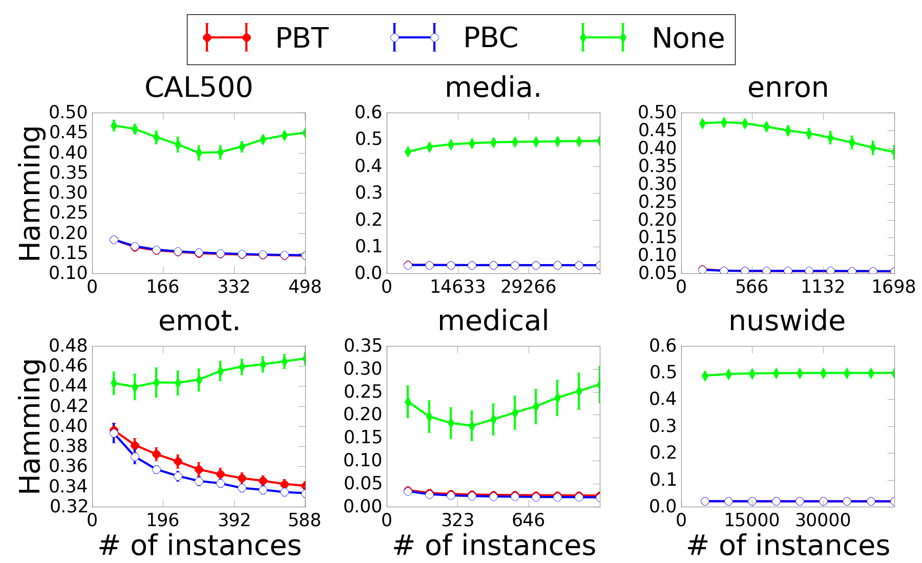
5.3 Experiments on Basis Drifting

To empirically justify the necessity of handling basis drifting, we compare variants of DPP that (a) incorporates PBC by (6), (b) incorporates PBT by (13), and (c) neglects basis drifting as (5). We plot the results for Hamming loss with M=10%M=10\% of KK in Figure 2 on six datasets, and report the complete results in Appendix B.2. The results on all datasets in Figure 2 show that DPP with either PBC or PBT significantly improves the performance over its variant that neglects the basis drifting, which clearly demonstrates the necessity to handle the drifting of projection basis.

Further comparison of PBC and PBT based on Figure 2 reveals that PBC in general performs slightly better than PBC, reflecting its advantage of exact projection basis correction. Nevertheless, as discussed in Section 5.2, PBT enjoys a nice computational speedup when KK and dd are large and MM is relatively small, making PBT more suitable to handle data with a large label set.

5.4 Experiments on Cost-Sensitivity

To empirically justify the necessity of cost-sensitivity, we compare CS-DPP using PBT with DPP using PBT and other online LSDR algorithms. To the best of our knowledge, no online LSDR algorithm has yet been proposed in the literature. We therefore design two simple online LSDR algorithms, online compressed sensing (O-CS) and online random projection (O-RAND), to compare with CS-DPP. O-CS is a straightforward extension of CS [13] with an online ridge regressor, and we follow [13] to determine the parameter of O-CS. O-RAND encodes using random matrix 𝐏R\mathbf{P}_{R} and simply decodes with the corresponding pseudo inverse 𝐏R†\mathbf{P}_{R}^{\dagger}.

We plot the results with respect to all evaluation criteria except for the Hamming loss with M=10%M=10\% of KK in Figure 3 on three datasets, and report the complete results in Appendix B.3 Note that the results for CS-DPP here are obtained by using the original label order from the dataset.

Refer to caption
Figure 3: CS-DPP vs. Others, M=10%M=10\% of KK

5.4.1 CS-DPP versus DPP.

The results of Figure 3 clearly indicate that CS-DPP performs significantly better than DPP on all evaluation criteria other than the Hamming loss, while CS-DPP reduces to DPP when cHam​(⋅,⋅)c_{\textsc{Ham}}(\cdot,\cdot) is used as the cost function. These observations demonstrate that CS-DPP, by optimizing the given cost function instead of Hamming loss, indeed achieves cost-sensitivity and is superior to its cost-insensitive counterpart, DPP.

5.4.2 CS-DPP versus Other Online LSDR Algorithms.

As shown in Figure 3, while DPP generally performs better than O-CS and O-RAND because of the advantage to preserve key label correlations rather than random ones, it can nevertheless be inferior on some datasets with respect to specific cost functions due to its cost-insensitivity. For example, DPP loses to O-RAND on dataset Corel5k with respect to the Normalized rank loss, as shown in the third row of Figure 3. CS-DPP conquers the weakness of DPP with its cost-sensitivity, and significantly outperforms O-CS and O-RAND on all three datasets with respect to all three evaluation criteria, as demonstrated in Figure 3. The superiority of CS-DPP justifies the necessity to take cost-sensitivity into account.

5.5 Experiment on Effect of Label Order for CS-DPP

10% of K 25% of K 50 % of K
chamc_{\textsc{ham}} 0.1458±0.000190.1458\pm 0.00019 0.1489±0.000120.1489\pm 0.00012 0.1503±0.000080.1503\pm 0.00008
cNRc_{\textsc{NR}} 0.1247±0.002240.1247\pm 0.00224 0.1321±0.002100.1321\pm 0.00210 0.1371±0.002220.1371\pm 0.00222
cF1c_{\textsc{F1}} 0.5914±0.001080.5914\pm 0.00108 0.5956±0.001100.5956\pm 0.00110 0.5949±0.001010.5949\pm 0.00101
cAccc_{\textsc{{Acc}}} 0.7388±0.001050.7388\pm 0.00105 0.7428±0.001310.7428\pm 0.00131 0.7426±0.001260.7426\pm 0.00126
Table 6: Results of CS-DPP on CAL500 with 50 random label orders
10% of K 25% of K 50 % of K
chamc_{\textsc{ham}} 0.2296±0.000100.2296\pm 0.00010 0.2162±0.000090.2162\pm 0.00009 0.2092±0.000010.2092\pm 0.00001
cNRc_{\textsc{NR}} 0.0064±0.000810.0064\pm 0.00081 0.0170±0.002420.0170\pm 0.00242 0.0232±0.001580.0232\pm 0.00158
cF1c_{\textsc{F1}} 0.4518±0.009190.4518\pm 0.00919 0.3841±0.001990.3841\pm 0.00199 0.3784±0.001070.3784\pm 0.00107
cAccc_{\textsc{{Acc}}} 0.5448±0.022520.5448\pm 0.02252 0.4971±0.003790.4971\pm 0.00379 0.4901±0.001240.4901\pm 0.00124
Table 7: Results of CS-DPP on yeast with 50 random label orders
10% of K 25% of K 50 % of K
chamc_{\textsc{ham}} 0.0562±0.000200.0562\pm 0.00020 0.0600±0.000110.0600\pm 0.00011 0.0632±0.000090.0632\pm 0.00009
cNRc_{\textsc{NR}} 0.1432±0.003330.1432\pm 0.00333 0.1364±0.002440.1364\pm 0.00244 0.1305±0.002160.1305\pm 0.00216
cF1c_{\textsc{F1}} 0.5421±0.003340.5421\pm 0.00334 0.5392±0.002910.5392\pm 0.00291 0.5428±0.002930.5428\pm 0.00293
cAccc_{\textsc{{Acc}}} 0.6573±0.003600.6573\pm 0.00360 0.6561±0.003310.6561\pm 0.00331 0.6627±0.003150.6627\pm 0.00315
Table 8: Results of CS-DPP on enron with 50 random label orders

The goal of this experiment is to study how different label orders affect the performance of CS-DPP as our proposed label weighting scheme with (14) is label-order-dependent. To evaluate the impact of label orders, we run CS-DPP with 5050 randomly generated label orders and M=10%M=10\%, 25%25\% and 50%50\% of KK on each dataset. The permutation of each dataset is fixed to the original one given in Mulan [30], which allows the variance of the performance to better indicate the effect of different orders.

We summarize the results of all four different cost functions with mean and standard deviation on datasets CAL500, enron and yeast in Table 8, 8 and 8 respectively, and report the complete results in Appendix B.4. Note that the results of Hamming loss are unaffected by the order of labels, and the reported deviation is due to the randomness from 𝐏t\mathbf{P}_{t}. From the results of Table 8, 8 and 8, we see that standard deviation is generally in a relatively small scale of 10−310^{-3}, indicating that the performance of CS-DPP is not that sensitive to the order of labels. Closer inspection of Table 8 reveals that the standard deviation of caccc_{\textsc{acc}} on yeast with M=10%M=10\% of KK (which is only 22 in this case) is somewhat larger, but for sufficiently large MM the label order does not seem to cause much variation.

6 Conclusion

We proposed a novel cost-sensitive online LSDR algorithm called cost-sensitive dynamic principal projection (CS-DPP). We established the foundation of CS-DPP with an online LSDR framework derived from PLST, and derived CS-DPP along with its theoretical guarantees on top of MSG. We successfully conquered the challenge of basis drifting using our carefully designed PBC and PBT. CS-DPP further achieves cost-sensitivity with theoretical guarantees based on our carefully designed label-weighting scheme. The empirical results demonstrate that CS-DPP significantly outperforms other OMLC algorithms on all evaluation criteria, which validates the robustness and superiority of CS-DPP. The necessity for CS-DPP to address LSDR, basis drifting and cost-sensitivity was also empirically justified.

For possible future works, an interesting direction is to design an online LSDR algorithm capable of capturing the key joint information between features and labels. As discussed, the concept to capture such joint information has been investigated for batch MLC [7, 17, 33], but it remains to be challenging for online MLC. Another direction is to apply OMLC algorithms as a fast approximate solver for large-scale batch data, and see how they compete with traditional batch algorithms. Another interesting direction, as mentioned in Section 2, is to design online learning algorithms that achieve cost-sensitivity for the more sophisticated micro- and macro-based criteria.

References

  • (1) Arora, R., Cotter, A., Srebro, N.: Stochastic optimization of PCA with capped MSG. In: NIPS 2013, pp. 1815–1823 (2013)
  • (2) Balasubramanian, K., Lebanon, G.: The landmark selection method for multiple output prediction. In: ICML 2012 (2012)
  • (3) Bartlett, P.: Online convex optimization: ridge regression, adaptivity (2008). URL https://people.eecs.berkeley.edu/~bartlett/courses/281b-sp08/24.pdf
  • (4) Bello, J.P., Chew, E., Turnbull, D.: Multilabel classification of music into emotions. In: ICMIR 2008, pp. 325–330 (2008)
  • (5) Bhatia, K., Jain, H., Kar, P., Varma, M., Jain, P.: Sparse local embeddings for extreme multi-label classification. In: NIPS 2015, pp. 730–738 (2015)
  • (6) Bi, W., Kwok, J.T.: Efficient multi-label classification with many labels. In: ICML 2013, pp. 405–413 (2013)
  • (7) Chen, Y., Lin, H.: Feature-aware label space dimension reduction for multi-label classification. In: NIPS 2012, pp. 1538–1546 (2012)
  • (8) Chua, T., Tang, J., Hong, R., Li, H., Luo, Z., Zheng, Y.: NUS-WIDE: a real-world web image database from national university of singapore. In: CIVR 2009 (2009)
  • (9) Crammer, K., Dekel, O., Keshet, J., S.-S., S., Singer, Y.: Online passive-aggressive algorithms. Journal of Machine Learning Research 7, 551–585 (2006)
  • (10) Dembczynski, K., Cheng, W., Hüllermeier, E.: Bayes optimal multilabel classification via probabilistic classifier chains. In: ICML 2010, pp. 279–286 (2010)
  • (11) Dembczynski, K., Waegeman, W., Cheng, W., Hüllermeier, E.: An exact algorithm for F-measure maximization. In: NIPS 2011, pp. 1404–1412 (2011)
  • (12) Elisseeff, A., Weston, J.: A kernel method for multilabelled classification. In: NIPS 2001 (2001)
  • (13) Hsu, D., Kakade, S., Langford, J., Zhang, T.: Multi-label prediction via compressed sensing. In: NIPS 2009, pp. 772–780 (2009)
  • (14) Kapoor, A., Viswanathan, R., Jain, P.: Multilabel classification using bayesian compressed sensing. In: NIPS 2012, pp. 2654–2662 (2012)
  • (15) Li, C., Lin, H.: Condensed filter tree for cost-sensitive multi-label classification. In: ICML 2014, pp. 423–431 (2014)
  • (16) Li, C., Lin, H., Lu, C.: Rivalry of two families of algorithms for memory-restricted streaming pca. In: AISTATS 2016 (2016)
  • (17) Lin, Z., Ding, G., Hu, M., Wang, J.: Multi-label classification via feature-aware implicit label space encoding. In: ICML 2014, pp. 325–333 (2014)
  • (18) Liu, W., Tsang, I.W., Müller, K.R.: An easy-to-hard learning paradigm for multiple classes and multiple labels. Journal of Machine Learning Research (2017)
  • (19) Lo, H., Wang, J., Wang, H., Lin, S.: Cost-sensitive multi-label learning for audio tag annotation and retrieval. IEEE Trans. Multimedia 13(3), 518–529 (2011)
  • (20) Mao, Q., Tsang, I.W.H., Gao, S.: Objective-guided image annotation. IEEE Transactions on Image Processing (2013)
  • (21) Nie, J., Kotlowski, W., Warmuth, M.K.: Online PCA with optimal regrets. Journal of Machine Learning Research 17, 194–200 (2016)
  • (22) Osojnik, A., Panov, P., Džeroski, S.: Multi-label classification via multi-target regression on data streams. Machine Learning (2017)
  • (23) Read, J., Bifet, A., Holmes, G., Pfahringer, B.: Streaming multi-label classification. In: Proceedings of the Workshop on Applications of Pattern Analysis (WAPA) 2011, pp. 19–25 (2011)
  • (24) Read, J., Pfahringer, B., Holmes, G., Frank, E.: Classifier chains for multi-label classification. Machine Learning 85(3), 333–359 (2011)
  • (25) Sun, L., Ji, S., Ye, J.: Canonical correlation analysis for multilabel classification: A least-squares formulation, extensions, and analysis. IEEE TPAMI 33(1), 194–200 (2011)
  • (26) Tai, F., Lin, H.: Multilabel classification with principal label space transformation. Neural Computation 24(9), 2508–2542 (2012)
  • (27) Tang, L., Rajan, S., Narayanan, V.K.: Large scale multi-label classification via metalabeler. In: WWW 2009, pp. 211–220 (2009)
  • (28) Tsoumakas, G., Katakis, I., Vlahavas, I.P.: Mining multi-label data. In: Data Mining and Knowledge Discovery Handbook, 2nd ed., pp. 667–685 (2010)
  • (29) Tsoumakas, G., Vlahavas, I.P.: Random k -labelsets: An ensemble method for multilabel classification. In: ECML 2007, pp. 406–417 (2007)
  • (30) Tsoumakas, G., Xioufis, E.S., Vilcek, J., Vlahavas, I.P.: MULAN: A java library for multi-label learning. Journal of Machine Learning Research 12, 2411–2414 (2011)
  • (31) Wu, Y., Lin, H.: Progressive kk-labelsets for cost-sensitive multi-label classification. Machine Learning (2016). Accepted for Special Issue of ACML 2016
  • (32) Xioufis, E.S., Spiliopoulou, M., Tsoumakas, G., Vlahavas, I.P.: Dealing with concept drift and class imbalance in multi-label stream classification. In: IJCAI 2011, pp. 1583–1588 (2011)
  • (33) Yu, H., Jain, P., Kar, P., Dhillon, I.S.: Large-scale multi-label learning with missing labels. In: ICML 2014, pp. 593–601 (2014)
  • (34) Zhang, X., Graepel, T., Herbrich, R.: Bayesian online learning for multi-label and multi-variate performance measures. In: AISTATS 2010 (2010)

Appendix A. Proof of Lemmas and Theorems

Appendix A.1 Proof of Lemma 1

Lemma 3

Suppose (𝐐t,σt)(\mathbf{Q}_{t},\sigma_{t}) is obtained after an updated of Capped MSG such that 𝐔t=𝐐t​diag​(σt)​𝐐t⊤\mathbf{U}_{t}=\mathbf{Q}_{t}\mbox{diag}(\sigma_{t})\mathbf{Q}_{t}^{\top}. If Γt\Gamma_{t} is a discrete probability distribution over events {𝐐t−i}i=1M+1\{\mathbf{Q}_{t}^{-i}\}_{i=1}^{M+1} with probability of 𝐐t−i\mathbf{Q}_{t}^{-i} being 1−σt​[i]1-\sigma_{t}[i], we have for any 𝐲\mathbf{y}

𝔼𝐏t∼Γt​[𝐲⊤​(𝐈−𝐏t⊤​𝐏t)​𝐲]=𝐲⊤​(𝐈−𝐔t)​𝐲\mathbb{E}_{\mathbf{P}_{t}\sim\Gamma_{t}}[\mathbf{y}^{\top}(\mathbf{I}-\mathbf{P}_{t}^{\top}\mathbf{P}_{t})\mathbf{y}]=\mathbf{y}^{\top}(\mathbf{I}-\mathbf{U}_{t})\mathbf{y} (16)
Proof

We first formally show that Γt\Gamma_{t} is a well-defined probability distribution. By the definition of the projection operator of Capped MSG we have 0≤σt​[i]≤10\leq\sigma_{t}[i]\leq 1 for each σt​[i]\sigma_{t}[i] and ∑i=1M+11−σt​[i]=M+1−∑i=1M+1σt​[i]=1\sum_{i=1}^{M+1}1-\sigma_{t}[i]=M+1-\sum_{i=1}^{M+1}\sigma_{t}[i]=1 with t​r​(𝐔t)=Mtr(\mathbf{U}_{t})=M. Γt\Gamma_{t} is therefore a well-defined probability distribution.

Then it suffices to show that 𝔼𝐏t∼Γt​[𝐏t⊤​𝐏t]=𝐔t\mathbb{E}_{\mathbf{P}_{t}\sim\Gamma_{t}}[\mathbf{P}_{t}^{\top}\mathbf{P}_{t}]=\mathbf{U}_{t} as

𝔼𝐏t∼Γt​[𝐲⊤​(𝐈−𝐏t⊤​𝐏t)​𝐲]=‖𝐲‖22−𝐲⊤​𝔼𝐏t∼Γt​[𝐏t⊤​𝐏t]​𝐲\mathbb{E}_{\mathbf{P}_{t}\sim\Gamma_{t}}[\mathbf{y}^{\top}(\mathbf{I}-\mathbf{P}_{t}^{\top}\mathbf{P}_{t})\mathbf{y}]=\|\mathbf{y}\|_{2}^{2}-\mathbf{y}^{\top}\mathbb{E}_{\mathbf{P}_{t}\sim\Gamma_{t}}[\mathbf{P}_{t}^{\top}\mathbf{P}_{t}]\mathbf{y}

To see that 𝔼𝐏t∼Γt​[𝐏t⊤​𝐏t]=𝐔t\mathbb{E}_{\mathbf{P}_{t}\sim\Gamma_{t}}[\mathbf{P}_{t}^{\top}\mathbf{P}_{t}]=\mathbf{U}_{t}, first notice that by orthogonality of rows of 𝐐t\mathbf{Q}_{t} we have 𝐔t=∑j=1M+1σt​(j)​𝐞j​𝐞j⊤\mathbf{U}_{t}=\sum_{j=1}^{M+1}\sigma_{t}(j)\mathbf{e}_{j}\mathbf{e}_{j}^{\top} where 𝐞j\mathbf{e}_{j} is the jj-th row of 𝐐t\mathbf{Q}_{t}. We then have

𝔼𝐏t∼Γt​[𝐏t⊤​𝐏t]\displaystyle\mathbb{E}_{\mathbf{P}_{t}\sim\Gamma_{t}}[\mathbf{P}_{t}^{\top}\mathbf{P}_{t}] =∑i=1M+1(1−σt[i])∑j=1M+1⟦i≠j⟧𝐞j𝐞j⊤\displaystyle=\sum_{i=1}^{M+1}(1-\sigma_{t}[i])\sum_{j=1}^{M+1}\llbracket i\neq j\rrbracket\mathbf{e}_{j}\mathbf{e}_{j}^{\top}
=∑j=1M+1(𝐞j𝐞j⊤∑i=1M+1⟦i≠j⟧(1−σt[i]))\displaystyle=\sum_{j=1}^{M+1}(\mathbf{e}_{j}\mathbf{e}_{j}^{\top}\sum_{i=1}^{M+1}\llbracket i\neq j\rrbracket(1-\sigma_{t}[i]))
=∑j=1M+1(σt​[j]​𝐞j​𝐞j⊤)\displaystyle=\sum_{j=1}^{M+1}(\sigma_{t}[j]\mathbf{e}_{j}\mathbf{e}_{j}^{\top}) (a)\displaystyle(a)
=𝐔t\displaystyle=\mathbf{U}_{t}

where (a)(a) is by ∑i=1M+1σt​[i]=M\sum_{i=1}^{M+1}\sigma_{t}[i]=M

Appendix A.2 Proof of Theorem 3.2

Theorem Appendix A..1

With the definitions of 𝐇t\mathbf{H}_{t} in (3.4.1), 𝐇∗\mathbf{H}^{*} in (9), ℛT\frac{\mathcal{R}}{T} in (8) and Δt\Delta_{t} in (10), assume that ‖𝐱t‖≤1\|\mathbf{x}_{t}\|\leq 1, ‖𝐲t‖≤1\|\mathbf{y}_{t}\|\leq 1 and ‖𝐇t​𝐱t−𝐲t‖22≤ϵ\|\mathbf{H}_{t}\mathbf{x}_{t}-\mathbf{y}_{t}\|_{2}^{2}\leq\epsilon.

  1. 1.

    For any given TT, the expected cumulative regret ℛ\mathcal{R} is upper-bounded by

    (1+ϵ)​∑t=1TΔt+M2​‖𝐇∗‖F2+2​ϵ​M​d​log⁡(1+Td).(1+\epsilon)\sum_{t=1}^{T}\Delta_{t}+\frac{M}{2}\|\mathbf{H}^{*}\|_{F}^{2}+2\epsilon Md\log\left(1+\frac{T}{d}\right).
  2. 2.

    If limT→∞ΔT=0\lim_{T\rightarrow\infty}\Delta_{T}=0 and ‖𝐇∗‖F≤h∗\|\mathbf{H}^{*}\|_{F}\leq h^{*} across all iterations, limT→∞ℛT=0\lim_{T\rightarrow\infty}\frac{\mathcal{R}}{T}=0.

Proof

We start by separating the definition of ℛ\mathcal{R} to two terms: one for how 𝐏t\mathbf{P}_{t} in MSG converges to 𝐏∗\mathbf{P}^{*}, and the other for how 𝐖tPBC\mathbf{W}_{t}^{\text{PBC}} for 𝐏t\mathbf{P}_{t} in ridge regression differs to 𝐖#\mathbf{W}_{\#} for 𝐏∗\mathbf{P}^{*}. For simplicity, we will denote 𝐖tPBC\mathbf{W}_{t}^{\text{PBC}} by 𝐖t\mathbf{W}_{t}. Then,

ℛ=\displaystyle\mathcal{R}= ∑t=1T𝔼𝐏t∼Γt​[ℓ(t)​(𝐖t,𝐏t)−ℓ(t)​(𝐖#,𝐏∗)]\displaystyle\sum_{t=1}^{T}\mathbb{E}_{\mathbf{P}_{t}\sim\Gamma_{t}}[\ell^{(t)}(\mathbf{W}_{t},\mathbf{P}_{t})-\ell^{(t)}(\mathbf{W}_{\#},\mathbf{P}^{*})]
=\displaystyle= +∑t=1T𝔼𝐏t∼Γt[∥𝐖t⊤𝐱t−𝐏t𝐲t∥22+∥(𝐈−𝐏t⊤𝐏t)𝐲t∥22]\displaystyle+\sum_{t=1}^{T}\mathbb{E}_{\mathbf{P}_{t}\sim\Gamma_{t}}[\|\mathbf{W}_{t}^{\top}\mathbf{x}_{t}-\mathbf{P}_{t}\mathbf{y}_{t}\|_{2}^{2}+\|(\mathbf{I}-\mathbf{P}_{t}^{\top}\mathbf{P}_{t})\mathbf{y}_{t}\|_{2}^{2}]
−∑t=1T𝔼𝐏t∼Γt[∥𝐖#⊤𝐱t−𝐏∗𝐲t∥22+∥(𝐈−(𝐏∗)⊤𝐏∗)𝐲t∥22]\displaystyle-\sum_{t=1}^{T}\mathbb{E}_{\mathbf{P}_{t}\sim\Gamma_{t}}[\|\mathbf{W}_{\#}^{\top}\mathbf{x}_{t}-\mathbf{P}^{*}\mathbf{y}_{t}\|_{2}^{2}+\|(\mathbf{I}-(\mathbf{P}^{*})^{\top}\mathbf{P}^{*})\mathbf{y}_{t}\|_{2}^{2}]
=\displaystyle= +∑t=1T𝔼𝐏t∼Γt[∥(𝐈−𝐏t⊤𝐏t)𝐲t∥22]−∥(𝐈−(𝐏∗)⊤𝐏∗)𝐲t∥22]⏟ℛMSG\displaystyle+\underbrace{\sum_{t=1}^{T}\mathbb{E}_{\mathbf{P}_{t}\sim\Gamma_{t}}[\|(\mathbf{I}-\mathbf{P}_{t}^{\top}\mathbf{P}_{t})\mathbf{y}_{t}\|_{2}^{2}]-\|(\mathbf{I}-(\mathbf{P}^{*})^{\top}\mathbf{P}^{*})\mathbf{y}_{t}\|_{2}^{2}]}_{\mathcal{R}_{\text{MSG}}}
+∑t=1T𝔼𝐏t∼Γt​[‖𝐖t⊤​𝐱t−𝐏t​𝐲t‖22]−‖𝐖#⊤​𝐱t−𝐏∗​𝐲t‖22⏟ℛridge\displaystyle+\underbrace{\sum_{t=1}^{T}\mathbb{E}_{\mathbf{P}_{t}\sim\Gamma_{t}}[\|\mathbf{W}_{t}^{\top}\mathbf{x}_{t}-\mathbf{P}_{t}\mathbf{y}_{t}\|_{2}^{2}]-\|\mathbf{W}_{\#}^{\top}\mathbf{x}_{t}-\mathbf{P}^{*}\mathbf{y}_{t}\|_{2}^{2}}_{\mathcal{R}_{\text{ridge}}}

We can bound ℛMSG\mathcal{R}_{\text{MSG}} first. Let 𝐔t=𝔼𝐏t∼Γt​[𝐏t⊤​𝐏t]\mathbf{U}_{t}=\mathbb{E}_{\mathbf{P}_{t}\sim\Gamma_{t}}[\mathbf{P}_{t}^{\top}\mathbf{P}_{t}] and 𝐔∗=(𝐏∗)⊤​𝐏∗\mathbf{U}^{*}=\left(\mathbf{P}^{*}\right)^{\top}\mathbf{P}^{*}, by linearity of expectation,

ℛMSG\displaystyle\mathcal{R}_{\text{MSG}} =∑t=1T𝐲t⊤​(𝐔t−𝐔∗)​𝐲t\displaystyle=\sum_{t=1}^{T}\mathbf{y}_{t}^{\top}(\mathbf{U}_{t}-\mathbf{U}^{*})\mathbf{y}_{t}
≤∑t=1T‖𝐔t−𝐔∗‖2\displaystyle\leq\sum_{t=1}^{T}\|\mathbf{U}_{t}-\mathbf{U}^{*}\|_{2} (17)
≤∑t=1TΔt\displaystyle\leq\sum_{t=1}^{T}\Delta_{t}

where (17) from the assumption of ‖𝐲t‖2≤1\|\mathbf{y}_{t}\|_{2}\leq 1 and the definition of the matrix 22-norm.

Next, we bound ℛridge\mathcal{R}_{\text{ridge}}. With the definitions of 𝐇t\mathbf{H}_{t} in (3.4.1) and 𝐇∗\mathbf{H}^{*} in (9), ℛridge\mathcal{R}_{\text{ridge}} can be further decomposed to

ℛridge=\displaystyle\mathcal{R}_{\text{ridge}}= +∑t=1T(𝔼𝐏t∼Γt​[‖𝐏t​(𝐇t⊤​𝐱t−𝐲t)‖22]−‖𝐏∗​(𝐇t⊤​𝐱t−𝐲t)‖22)⏟ℛ1\displaystyle+\underbrace{\sum_{t=1}^{T}\left(\mathbb{E}_{\mathbf{P}_{t}\sim\Gamma_{t}}[\|\mathbf{P}_{t}(\mathbf{H}_{t}^{\top}\mathbf{x}_{t}-\mathbf{y}_{t})\|_{2}^{2}]-\|\mathbf{P}^{*}(\mathbf{H}_{t}^{\top}\mathbf{x}_{t}-\mathbf{y}_{t})\|_{2}^{2}\right)}_{\mathcal{R}_{1}}
+∑t=1T(‖𝐏∗​(𝐇t⊤​𝐱t−𝐲t)‖22−‖𝐏∗​((𝐇∗)⊤​𝐱t−𝐲t)‖22)⏟ℛ2.\displaystyle+\underbrace{\sum_{t=1}^{T}\left(\|\mathbf{P}^{*}(\mathbf{H}_{t}^{\top}\mathbf{x}_{t}-\mathbf{y}_{t})\|_{2}^{2}-\|\mathbf{P}^{*}(\left(\mathbf{H}^{*}\right)^{\top}\mathbf{x}_{t}-\mathbf{y}_{t})\|_{2}^{2}\right)}_{\mathcal{R}_{2}}.

Bounding ℛ1\mathcal{R}_{1} is very similar to bounding ℛMSG\mathcal{R}_{\text{MSG}}. In particular,

ℛ1\displaystyle\mathcal{R}_{1} =∑t=1T(𝐇t⊤​𝐱t−𝐲t)⊤​(𝐔t−𝐔∗)​(𝐇t⊤​𝐱t−𝐲t)\displaystyle=\sum_{t=1}^{T}(\mathbf{H}_{t}^{\top}\mathbf{x}_{t}-\mathbf{y}_{t})^{\top}(\mathbf{U}_{t}-\mathbf{U}^{*})(\mathbf{H}_{t}^{\top}\mathbf{x}_{t}-\mathbf{y}_{t})
≤∑t=1Tϵ​‖𝐔t−𝐔∗‖2\displaystyle\leq\sum_{t=1}^{T}\epsilon\|\mathbf{U}_{t}-\mathbf{U}^{*}\|_{2} (18)
≤∑t=1Tϵ​Δt\displaystyle\leq\sum_{t=1}^{T}\epsilon\Delta_{t}

where (18) follows from the assumption of ‖𝐇t⊤​𝐱t−𝐲t‖22≤ϵ\|\mathbf{H}_{t}^{\top}\mathbf{x}_{t}-\mathbf{y}_{t}\|_{2}^{2}\leq\epsilon.

The term ℛ2\mathcal{R}_{2} can be viewed as an online ridge regression process from 𝐱\mathbf{x} to 𝐏∗​𝐲\mathbf{P}^{*}\mathbf{y}, because it can be easily proved that 𝐇t​(𝐏∗)⊤\mathbf{H}_{t}(\mathbf{P}^{*})^{\top} is the ridge regression solution after receiving (𝐱1,𝐏∗​𝐲1)(\mathbf{x}_{1},\mathbf{P}^{*}\mathbf{y}_{1}), (𝐱2,𝐏∗​𝐲2)(\mathbf{x}_{2},\mathbf{P}^{*}\mathbf{y}_{2}), …\ldots, (𝐱t−1,𝐏∗​𝐲t−1)(\mathbf{x}_{t-1},\mathbf{P}^{*}\mathbf{y}_{t-1}). Also, as discussed in Section 3.4, 𝐖#=𝐇∗​(𝐏∗)⊤\mathbf{W}_{\#}=\mathbf{H}^{*}(\mathbf{P}^{*})^{\top} is the optimal linear regression solution of {(𝐱t,𝐏∗​𝐲t)}t=1T\{(\mathbf{x}_{t},\mathbf{P}^{*}\mathbf{y}_{t})\}_{t=1}^{T}. The assumption of ‖𝐇t​𝐱t−𝐲t‖22≤ϵ\|\mathbf{H}_{t}\mathbf{x}_{t}-\mathbf{y}_{t}\|_{2}^{2}\leq\epsilon implies that

‖𝐏∗​𝐇t⊤​𝐱t−𝐏∗​𝐲t‖22=(𝐇t⊤​𝐱t−𝐲t)⊤​𝐔∗​(𝐇t⊤​𝐱t−𝐲t)≤ϵ\displaystyle\|\mathbf{P}^{*}\mathbf{H}_{t}^{\top}\mathbf{x}_{t}-\mathbf{P}^{*}\mathbf{y}_{t}\|_{2}^{2}=(\mathbf{H}_{t}^{\top}\mathbf{x}_{t}-\mathbf{y}_{t})^{\top}\mathbf{U}^{*}(\mathbf{H}_{t}^{\top}\mathbf{x}_{t}-\mathbf{y}_{t})\leq\epsilon

as well. Similarly, he assumption of ‖𝐲t‖2≤1\|\mathbf{y}_{t}\|_{2}\leq 1 implies that ‖𝐏∗​yt‖2≤1\|\mathbf{P}^{*}y_{t}\|_{2}\leq 1. Then, a standard ridge regression analysis (see, e.g. [3]) by provng that 𝐀t=λ​𝐈+∑i=1t−1𝐱i​𝐱i⊤\mathbf{A}_{t}=\lambda\mathbf{I}+\sum_{i=1}^{t-1}\mathbf{x}_{i}\mathbf{x}_{i}^{\top} grows linearly with tt leads to

ℛ2\displaystyle\mathcal{R}_{2} =∑t=1T(‖𝐏∗​(𝐇t⊤​𝐱t−𝐲t)‖22−‖𝐏∗​((𝐇∗)⊤​𝐱t−𝐲t)‖22)\displaystyle=\sum_{t=1}^{T}\left(\|\mathbf{P}^{*}(\mathbf{H}_{t}^{\top}\mathbf{x}_{t}-\mathbf{y}_{t})\|_{2}^{2}-\|\mathbf{P}^{*}(\left(\mathbf{H}^{*}\right)^{\top}\mathbf{x}_{t}-\mathbf{y}_{t})\|_{2}^{2}\right)
≤12​‖𝐏∗​𝐇∗‖F2+2​ϵ​M​d​log⁡(1+Td)\displaystyle\leq\frac{1}{2}\|\mathbf{P}^{*}\mathbf{H}^{*}\|_{F}^{2}+2\epsilon Md\log\left(1+\frac{T}{d}\right)
≤M2​‖𝐇∗‖F2+2​ϵ​M​d​log⁡(1+Td)\displaystyle\leq\frac{M}{2}\|\mathbf{H}^{*}\|_{F}^{2}+2\epsilon Md\log\left(1+\frac{T}{d}\right) (19)

where (19) is because ‖𝐏∗‖F2=t​r​(𝐔∗)=M\|\mathbf{P}^{*}\|_{F}^{2}=tr(\mathbf{U}^{*})=M.

Summing ℛMSG\mathcal{R}_{\text{MSG}}, ℛ1\mathcal{R}_{1} and ℛ2\mathcal{R}_{2} results in

ℛ≤(1+ϵ)​∑t=1TΔt+M2​‖𝐇∗‖F2+2​ϵ​M​d​log⁡(1+Td),\displaystyle\mathcal{R}\leq(1+\epsilon)\sum_{t=1}^{T}\Delta_{t}+\frac{M}{2}\|\mathbf{H}^{*}\|_{F}^{2}+2\epsilon Md\log(1+\frac{T}{d}), (20)

which proves the first part of the theorem. The second part easily follows because the convergence of a sequence implies the convergence of the mean.

Appendix A.3 Proof of Lemma 2

Lemma 4

If c⁡(𝐲,𝐲pred(k))−c⁡(𝐲,𝐲real(k))≥0c(\mathbf{y},\mathbf{y}^{(k)}_{\text{pred}})-c(\mathbf{y},\mathbf{y}^{(k)}_{\text{real}})\geq 0 holds for any kk, 𝐲\mathbf{y} and 𝐲^\hat{\mathbf{y}}, then for any given 𝐲\mathbf{y} and 𝐲^\hat{\mathbf{y}} we have

c(𝐲,𝐲^)=∑k=1Kδ(k)⟦𝐲[k]≠𝐲^[k]⟧c(\mathbf{y},\hat{\mathbf{y}})=\sum_{k=1}^{K}\delta^{(k)}\llbracket\mathbf{y}[k]\neq\hat{\mathbf{y}}[k]\rrbracket (21)
Proof

Recall the definition of 𝐲real(k)\mathbf{y}^{(k)}_{\text{real}} and 𝐲(k)pred\mathbf{y}^{(k)_{\text{pred}}} to be

𝐲^real(k)​[i]={𝐲⁡[i]if​i≤k𝐲^​[i]if​i>k​and​𝐲^pred(k)​[i]={𝐲⁡[i]if​i<k𝐲^​[i]if​i≥k\hat{\mathbf{y}}_{\text{real}}^{(k)}[i]=\begin{cases}\mathbf{y}[i]&\text{if}\,i\leq k\\ \hat{\mathbf{y}}[i]&\text{if}\,i>k\\ \end{cases}\>\text{{and}}\>\hat{\mathbf{y}}_{\text{pred}}^{(k)}[i]=\begin{cases}\mathbf{y}[i]&\text{if}\,i<k\\ \hat{\mathbf{y}}[i]&\text{if}\,i\geq k\\ \end{cases}

and the definition of δ(k)\delta^{(k)} to be

δ(k)=|c⁡(𝐲,𝐲^pred(k))−c⁡(𝐲,𝐲^real(k))|\delta^{(k)}=|c(\mathbf{y},\hat{\mathbf{y}}_{\text{pred}}^{(k)})-c(\mathbf{y},\hat{\mathbf{y}}_{\text{real}}^{(k)})|

Now define ki,i=1,…,Lk_{i},i=1,\ldots,L be the sequence of indices such that 𝐲⁡[ki]≠𝐲^​[ki]\mathbf{y}[k_{i}]\neq\hat{\mathbf{y}}[k_{i}] for every kik_{i} and ki<ki+1k_{i}<k_{i+1}. If such kik_{i} does not exist than (21) holds trivially by c⁡(𝐲,𝐲)=0c(\mathbf{y},\mathbf{y})=0. Otherwise, by the condition of cc we have

∑k=1Kδ(k)⟦𝐲[k]≠𝐲^[k]⟧\displaystyle\sum_{k=1}^{K}\delta^{(k)}\llbracket\mathbf{y}[k]\neq\hat{\mathbf{y}}[k]\rrbracket (a)\displaystyle(a)
=\displaystyle= ∑k=1K(c(𝐲,𝐲^pred(k))−c(𝐲,𝐲^real(k)))⟦𝐲[k]≠𝐲^[k]⟧\displaystyle\sum_{k=1}^{K}(c(\mathbf{y},\hat{\mathbf{y}}_{\text{pred}}^{(k)})-c(\mathbf{y},\hat{\mathbf{y}}_{\text{real}}^{(k)}))\llbracket\mathbf{y}[k]\neq\hat{\mathbf{y}}[k]\rrbracket
=\displaystyle= ∑i=1Lc⁡(𝐲,𝐲^pred(ki))−c⁡(𝐲,𝐲^real(ki))\displaystyle\sum_{i=1}^{L}c(\mathbf{y},\hat{\mathbf{y}}_{\text{pred}}^{(k_{i})})-c(\mathbf{y},\hat{\mathbf{y}}_{\text{real}}^{(k_{i})})
=\displaystyle= c⁡(𝐲,𝐲^pred(k1))−c⁡(𝐲,𝐲^real(kL))\displaystyle c(\mathbf{y},\hat{\mathbf{y}}_{\text{pred}}^{(k_{1})})-c(\mathbf{y},\hat{\mathbf{y}}_{\text{real}}^{(k_{L})}) (b)\displaystyle(b)
=\displaystyle= c⁡(𝐲,𝐲^)\displaystyle c(\mathbf{y},\hat{\mathbf{y}}) (c)\displaystyle(c)

where (a)(a) uses the condition of c⁡(⋅,⋅)c(\cdot,\cdot) to remove the absolute value function; (b)(b) is from two possibilities of LL: if L=1L=1 then the equation trivially holds; if L>1L>1 we use the observation that 𝐲^real(ki)=𝐲^pred(ki+1)\hat{\mathbf{y}}_{\text{real}}^{(k_{i})}=\hat{\mathbf{y}}_{\text{pred}}^{(k_{i+1})} where the observation is by realizing 𝐲​[j]=𝐲^​[j]\mathbf{y}[j]=\hat{\mathbf{y}}[j] for any ki<j<ki+1k_{i}<j<k_{i+1}; (c)(c) follows from the observation that 𝐲^pred(k1)=𝐲^\hat{\mathbf{y}}^{(k_{1})}_{\text{pred}}=\hat{\mathbf{y}} and 𝐲^real(kL)=𝐲\hat{\mathbf{y}}^{(k_{L})}_{\text{real}}=\mathbf{y} and c⁡(𝐲,𝐲)=0c(\mathbf{y},\mathbf{y})=0.

Appendix A.4 Proof of Theorem 4.1

Theorem Appendix A..2

When making a prediction 𝐲^\hat{\mathbf{y}} from 𝐱\mathbf{x} by 𝐲^=round⁡(𝐏⊤​𝐫​(𝐱)+𝐨)\hat{\mathbf{y}}=\mathrm{round}\left(\mathbf{P}^{\top}\mathbf{r}(\mathbf{x})+\mathbf{o}\right) with any left orthogonal matrix 𝐏\mathbf{P}, if c⁡(⋅,⋅)c(\cdot,\cdot) satisfies the condition of Lemma 2, the prediction cost

c⁡(𝐲,𝐲^)≤‖𝐫⁡(𝐱)−𝐳𝐂‖22+‖(𝐈−𝐏⊤​𝐏)​(𝐲𝐂′)‖22c(\mathbf{y},\hat{\mathbf{y}})\leq\|\mathbf{r}(\mathbf{x})-\mathbf{z}_{\mathbf{C}}\|^{2}_{2}+\|(\mathbf{I}-\mathbf{P}^{\top}\mathbf{P})(\mathbf{y}_{\mathbf{C}}^{\prime})\|^{2}_{2}

where 𝐳𝐂=𝐏⁡(𝐲𝐂′)\mathbf{z}_{\mathbf{C}}=\mathbf{P}(\mathbf{y}_{\mathbf{C}}^{\prime}) and 𝐲𝐂′=𝐂𝐲−𝐨\mathbf{y}_{\mathbf{C}}^{\prime}=\mathbf{C}\mathbf{y}-\mathbf{o} with respect to any fixed reference point 𝐨\mathbf{o}.

Recall the definition of 𝐂\mathbf{C} in the main context is

𝐂=diag​(δ(1),…,δ(K))\mathbf{C}=\mbox{diag}(\sqrt{\delta^{(1)}},...,\sqrt{\delta^{(K)}}) (22)

Next we show and prove the following lemma before we proceed to the complete proof.

Lemma 5

Given the ground truth 𝐲\mathbf{y}, if the binary-value prediction 𝐲^∈{+1,−1}K\hat{\mathbf{y}}\in\{+1,-1\}^{K} is made by round⁡(𝐲~)\mathrm{round}(\tilde{\mathbf{y}}) where 𝐲~\tilde{\mathbf{y}} is the real-value prediction 𝐲~∈ℝK\tilde{\mathbf{y}}\in\mathbb{R}^{K}. Then for any 𝐲\mathbf{y}, 𝐲^\hat{\mathbf{y}}, 𝐲~\tilde{\mathbf{y}}, if cc satisfies the condition in Lemma 2, we have

c⁡(𝐲,𝐲^)≤‖𝐂𝐲−𝐲~‖2c(\mathbf{y},\hat{\mathbf{y}})\leq\|\mathbf{C}\mathbf{y}-\tilde{\mathbf{y}}\|^{2} (23)
Proof

From Lemma 2 we have c(𝐲,𝐲^)=∑k=1Kδ(k)⟦𝐲[k]≠𝐲^[k]⟧c(\mathbf{y},\hat{\mathbf{y}})=\sum_{k=1}^{K}\delta^{(k)}\llbracket\mathbf{y}[k]\neq\hat{\mathbf{y}}[k]\rrbracket. As ‖𝐂𝐲−𝐲~‖22=∑k=1K(δ(K)​𝐲​[k]−𝐲~​[k])2\|\mathbf{C}\mathbf{y}-\tilde{\mathbf{y}}\|_{2}^{2}=\sum_{k=1}^{K}(\sqrt{\delta^{(K)}}\mathbf{y}[k]-\tilde{\mathbf{y}}[k])^{2}, it suffices to show that for all kk we have

δ(k)⟦𝐲[k]≠𝐲^[k]⟧≤(δ(k)𝐲[k]−𝐲~[k])2\delta^{(k)}\llbracket\mathbf{y}[k]\neq\hat{\mathbf{y}}[k]\rrbracket\leq(\sqrt{\delta^{(k)}}\mathbf{y}[k]-\tilde{\mathbf{y}}[k])^{2} (24)

When δ(k)=0\delta^{(k)}=0, (24) holds trivially. When δ(k)>0\delta^{(k)}>0, we have

δ(k)⟦𝐲[k]≠𝐲^[k]⟧\displaystyle\delta^{(k)}\llbracket\mathbf{y}[k]\neq\hat{\mathbf{y}}[k]\rrbracket
=\displaystyle= δ(k)(⟦𝐲~[k]≥0⟧⟦𝐲[k]=−1⟧+⟦𝐲~[k]<0⟧⟦𝐲[k]=+1⟧)\displaystyle\delta^{(k)}(\llbracket\tilde{\mathbf{y}}[k]\geq 0\rrbracket\llbracket\mathbf{y}[k]=-1\rrbracket+\llbracket\tilde{\mathbf{y}}[k]<0\rrbracket\llbracket\mathbf{y}[k]=+1\rrbracket)
=\displaystyle= δ(k)(⟦𝐲~​[k]δ(k)≥0⟧⟦𝐲[k]=−1⟧+⟦𝐲~​[k]δ(k)<0⟧⟦𝐲[k]=+1⟧)\displaystyle\delta^{(k)}(\llbracket\frac{\tilde{\mathbf{y}}[k]}{\sqrt{\delta^{(k)}}}\geq 0\rrbracket\llbracket\mathbf{y}[k]=-1\rrbracket+\llbracket\frac{\tilde{\mathbf{y}}[k]}{\sqrt{\delta^{(k)}}}<0\rrbracket\llbracket\mathbf{y}[k]=+1\rrbracket)
≤\displaystyle\leq δ(k)((𝐲~​[k]δ(k)−𝐲[k])2⟦𝐲[k]=−1⟧+(𝐲~​[k]δ(k)−𝐲[k])2⟦𝐲[k]=+1⟧)\displaystyle\delta^{(k)}((\frac{\tilde{\mathbf{y}}[k]}{\sqrt{\delta^{(k)}}}-\mathbf{y}[k])^{2}\llbracket\mathbf{y}[k]=-1\rrbracket+(\frac{\tilde{\mathbf{y}}[k]}{\sqrt{\delta^{(k)}}}-\mathbf{y}[k])^{2}\llbracket\mathbf{y}[k]=+1\rrbracket)
=\displaystyle= δ(k)​(𝐲~​[k]δ(k)−𝐲⁡[k])2\displaystyle\delta^{(k)}(\frac{\tilde{\mathbf{y}}[k]}{\sqrt{\delta^{(k)}}}-\mathbf{y}[k])^{2}
=\displaystyle= (δ(k)​𝐲​[k]−𝐲~​[k])2\displaystyle(\sqrt{\delta^{(k)}}\mathbf{y}[k]-\tilde{\mathbf{y}}[k])^{2}

where the second equality uses the fact that δ(k)>0\delta^{(k)}>0. As δ(k)≥0\delta^{(k)}\geq 0 holds by its definition, (24) holds for every kk. Summing (24) with respect to all kk then completes the proof.

With Lemma 5 established, we now prove Theorem 4.1.

Proof (Proof of Theorem 4.1)

If the given cc satisfies the condition in Lemma (2), and let 𝐲~=𝐏⊤​𝐫​(𝐱)+𝐨\tilde{\mathbf{y}}=\mathbf{P}^{\top}\mathbf{r}(\mathbf{x})+\mathbf{o} and 𝐲^=round⁡(𝐲~)\hat{\mathbf{y}}=\mathrm{round}(\tilde{\mathbf{y}}). Then for any (𝐱,𝐲)(\mathbf{x},\mathbf{y}) we have

c⁡(𝐲,𝐲^)\displaystyle c(\mathbf{y},\hat{\mathbf{y}})
≤\displaystyle\leq ‖𝐂𝐲−𝐲~‖22\displaystyle\|\mathbf{C}\mathbf{y}-\tilde{\mathbf{y}}\|^{2}_{2} (a)\displaystyle(a)
=\displaystyle= ‖((𝐲~−𝐨−𝐏⊤​𝐏𝐲𝐂′)−(𝐲𝐂′−𝐏⊤​𝐏𝐲𝐂′))‖22\displaystyle\|((\tilde{\mathbf{y}}-\mathbf{o}-\mathbf{P}^{\top}\mathbf{P}\mathbf{y}_{\mathbf{C}}^{\prime})-(\mathbf{y}_{\mathbf{C}}^{\prime}-\mathbf{P}^{\top}\mathbf{P}\mathbf{y}_{\mathbf{C}}^{\prime}))\|^{2}_{2}
=\displaystyle= ∥(𝐏⊤(𝐫(𝐱)−𝐳𝐂)−(𝐈−𝐏⊤𝐏)𝐲𝐂′∥22\displaystyle\|(\mathbf{P}^{\top}(\mathbf{r}(\mathbf{x})-\mathbf{z}^{\mathbf{C}})-(\mathbf{I}-\mathbf{P}^{\top}\mathbf{P})\mathbf{y}_{\mathbf{C}}^{\prime}\|^{2}_{2}
=\displaystyle= ∥(𝐏⊤(𝐫(𝐱)−𝐳𝐂)∥22+∥(𝐈−𝐏⊤𝐏)𝐲𝐂′)∥22\displaystyle\|(\mathbf{P}^{\top}(\mathbf{r}(\mathbf{x})-\mathbf{z}^{\mathbf{C}})\|^{2}_{2}+\|(\mathbf{I}-\mathbf{P}^{\top}\mathbf{P})\mathbf{y}_{\mathbf{C}}^{\prime})\|^{2}_{2} (b)\displaystyle(b)
=\displaystyle= ‖𝐫⁡(𝐱)−𝐳𝐂‖22+‖(𝐈−𝐏⊤​𝐏)​𝐲𝐂′‖22\displaystyle\|\mathbf{r}(\mathbf{x})-\mathbf{z}_{\mathbf{C}}\|^{2}_{2}+\|(\mathbf{I}-\mathbf{P}^{\top}\mathbf{P})\mathbf{y}_{\mathbf{C}}^{\prime}\|^{2}_{2} (c)\displaystyle(c)

where we recall that 𝐲¯𝐂′=𝐂𝐲−𝐨\bar{\mathbf{y}}_{\mathbf{C}}^{\prime}=\mathbf{C}\mathbf{y}-\mathbf{o} and 𝐳𝐂=𝐏⁡(𝐲𝐜′)\mathbf{z}_{\mathbf{C}}=\mathbf{P}(\mathbf{y}_{\mathbf{c}}^{\prime}). (a)(a) is from Lemma 24, while (b)(b) and (c)(c) follow from the orthogonal rows of 𝐏\mathbf{P}.

We note that the proof above closely follows the proof of Theorem 1 in [26], while the key difference comes from Lemma 5 to handle the weighted Hamming loss.

Appendix B. Complete Results of Experiments

Here we report the complete results of each experiment.

Appendix B.1 Necessity of Online LSDR

We report the complete results of comparison between O-BR and DPP with M=10%M=10\%, 25%25\% and 50%50\% of KK from Table 9 to Table 11 with respect to all four evaluation criteria, where the best values (the lowest) are marked in bold.

The results show that DPP outperforms O-BR as the value of pp increases with respect to Hamming loss, F1 loss and Accuracy loss, demonstrating the robustness of DPP. On the otter hand, the results related to Normalized rank loss from Table 9 to Table 11 show that, while DPP cannot outperform O-BR regarding this specific criterion, DPP does start to perform competitively as the value of pp increases. The observation again demonstrates that DPP indeed suffers less from noisy labels comparing to O-BR due to the incorporation with LSDR.

𝖣𝖺𝗍𝖺𝗌𝖾𝗍\mathsf{Dataset} 𝖠𝗅𝗀.\mathsf{Alg.} 𝖧𝖺𝗆𝗆.𝗅𝗈𝗌𝗌\mathsf{Hamm.\,loss} 𝖥𝟣​𝗅𝗈𝗌𝗌\mathsf{F1\,loss} 𝖠𝖼𝖼.𝗅𝗈𝗌𝗌\mathsf{Acc.\,loss} 𝖭𝗈𝗋𝗆.𝗋𝖺𝗇𝗄​𝗅𝗈𝗌𝗌\mathsf{Norm.\,rank\,loss}
𝖢𝖠𝖫𝟧𝟢𝟢\mathsf{CAL500} O-BR 0.1130±0.0003{0.1130\pm 0.0003} 0.823±0.002\mathbf{0.823\pm 0.002} 0.453±0.001\mathbf{0.453\pm 0.001} 0.898±0.001\mathbf{0.898\pm 0.001}
DPP-50 0.1143±0.0001{0.1143\pm 0.0001} 0.823±0.002\mathbf{0.823\pm 0.002} 0.455±0.001{0.455\pm 0.001} 0.897±0.001\mathbf{0.897\pm 0.001}
DPP-25 0.1133±0.0002{0.1133\pm 0.0002} 0.830±0.003{0.830\pm 0.003} 0.454±0.001{0.454\pm 0.001} 0.900±0.001\mathbf{0.900\pm 0.001}
DPP-10 0.1113±0.0002\mathbf{0.1113\pm 0.0002} 0.837±0.002{0.837\pm 0.002} 0.458±0.001{0.458\pm 0.001} 0.911±0.002{0.911\pm 0.002}
𝖢𝗈𝗋𝖾𝗅𝟧𝗄\mathsf{Corel5k} O-BR 0.0070±0.0000\mathbf{0.0070\pm 0.0000} 0.949±0.001{0.949\pm 0.001} 0.496±0.000\mathbf{0.496\pm 0.000} 0.957±0.001\mathbf{0.957\pm 0.001}
DPP-50 0.0072±0.0000{0.0072\pm 0.0000} 0.945±0.001\mathbf{0.945\pm 0.001} 0.496±0.001\mathbf{0.496\pm 0.001} 0.957±0.001\mathbf{0.957\pm 0.001}
DPP-25 0.0072±0.0000{0.0072\pm 0.0000} 0.949±0.001{0.949\pm 0.001} 0.497±0.000\mathbf{0.497\pm 0.000} 0.958±0.000\mathbf{0.958\pm 0.000}
DPP-10 0.0071±0.0000{0.0071\pm 0.0000} 0.949±0.001{0.949\pm 0.001} 0.498±0.000{0.498\pm 0.000} 0.960±0.001{0.960\pm 0.001}
𝖾𝗆𝗈𝗍𝗂𝗈𝗇𝗌\mathsf{emotions} O-BR 0.2213±0.0011\mathbf{0.2213\pm 0.0011} 0.697±0.005\mathbf{0.697\pm 0.005} 0.480±0.004\mathbf{0.480\pm 0.004} 0.719±0.005\mathbf{0.719\pm 0.005}
DPP-50 0.2214±0.0013\mathbf{0.2214\pm 0.0013} 0.740±0.008{0.740\pm 0.008} 0.504±0.005{0.504\pm 0.005} 0.764±0.004{0.764\pm 0.004}
DPP-25 0.2226±0.0013\mathbf{0.2226\pm 0.0013} 0.767±0.006{0.767\pm 0.006} 0.527±0.003{0.527\pm 0.003} 0.783±0.002{0.783\pm 0.002}
DPP-10 0.2238±0.0026\mathbf{0.2238\pm 0.0026} 0.857±0.003{0.857\pm 0.003} 0.570±0.002{0.570\pm 0.002} 0.858±0.004{0.858\pm 0.004}
𝖾𝗇𝗋𝗈𝗇\mathsf{enron} O-BR 0.0584±0.0002{0.0584\pm 0.0002} 0.694±0.002\mathbf{0.694\pm 0.002} 0.386±0.001\mathbf{0.386\pm 0.001} 0.766±0.002\mathbf{0.766\pm 0.002}
DPP-50 0.0572±0.0002{0.0572\pm 0.0002} 0.697±0.003\mathbf{0.697\pm 0.003} 0.388±0.001\mathbf{0.388\pm 0.001} 0.770±0.002\mathbf{0.770\pm 0.002}
DPP-25 0.0534±0.0002{0.0534\pm 0.0002} 0.696±0.002\mathbf{0.696\pm 0.002} 0.397±0.001{0.397\pm 0.001} 0.767±0.002\mathbf{0.767\pm 0.002}
DPP-10 0.0489±0.0001\mathbf{0.0489\pm 0.0001} 0.716±0.002{0.716\pm 0.002} 0.414±0.001{0.414\pm 0.001} 0.784±0.002{0.784\pm 0.002}
𝗆𝖾𝖽𝗂𝖺𝗆𝗂𝗅𝗅\mathsf{mediamill} O-BR 0.0271±0.0000\mathbf{0.0271\pm 0.0000} 0.640±0.001\mathbf{0.640\pm 0.001} 0.403±0.000\mathbf{0.403\pm 0.000} 0.721±0.000\mathbf{0.721\pm 0.000}
DPP-50 0.0272±0.0000{0.0272\pm 0.0000} 0.640±0.001\mathbf{0.640\pm 0.001} 0.402±0.000\mathbf{0.402\pm 0.000} 0.721±0.000\mathbf{0.721\pm 0.000}
DPP-25 0.0272±0.0000{0.0272\pm 0.0000} 0.639±0.001\mathbf{0.639\pm 0.001} 0.403±0.000\mathbf{0.403\pm 0.000} 0.721±0.001\mathbf{0.721\pm 0.001}
DPP-10 0.0272±0.0000{0.0272\pm 0.0000} 0.639±0.001\mathbf{0.639\pm 0.001} 0.402±0.000\mathbf{0.402\pm 0.000} 0.720±0.001\mathbf{0.720\pm 0.001}
𝗆𝖾𝖽𝗂𝖼𝖺𝗅\mathsf{medical} O-BR 0.0168±0.0001\mathbf{0.0168\pm 0.0001} 0.550±0.004\mathbf{0.550\pm 0.004} 0.448±0.004\mathbf{0.448\pm 0.004} 0.563±0.005\mathbf{0.563\pm 0.005}
DPP-50 0.0177±0.0001{0.0177\pm 0.0001} 0.544±0.006\mathbf{0.544\pm 0.006} 0.446±0.002\mathbf{0.446\pm 0.002} 0.556±0.003\mathbf{0.556\pm 0.003}
DPP-25 0.0183±0.0001{0.0183\pm 0.0001} 0.577±0.004{0.577\pm 0.004} 0.469±0.005{0.469\pm 0.005} 0.589±0.005{0.589\pm 0.005}
DPP-10 0.0190±0.0001{0.0190\pm 0.0001} 0.645±0.006{0.645\pm 0.006} 0.538±0.003{0.538\pm 0.003} 0.651±0.004{0.651\pm 0.004}
𝗇𝗎𝗌𝗐𝗂𝖽𝖾\mathsf{nuswide} O-BR 0.0151±0.0000\mathbf{0.0151\pm 0.0000} 0.627±0.001\mathbf{0.627\pm 0.001} 0.668±0.000\mathbf{0.668\pm 0.000} 0.632±0.000{0.632\pm 0.000}
DPP-50 0.0151±0.0000{0.0151\pm 0.0000} 0.627±0.000\mathbf{0.627\pm 0.000} 0.667±0.000\mathbf{0.667\pm 0.000} 0.633±0.000{0.633\pm 0.000}
DPP-25 0.0151±0.0000{0.0151\pm 0.0000} 0.627±0.000\mathbf{0.627\pm 0.000} 0.667±0.000\mathbf{0.667\pm 0.000} 0.632±0.000\mathbf{0.632\pm 0.000}
DPP-10 0.0151±0.0000{0.0151\pm 0.0000} 0.626±0.000\mathbf{0.626\pm 0.000} 0.668±0.000\mathbf{0.668\pm 0.000} 0.632±0.000{0.632\pm 0.000}
𝗌𝖼𝖾𝗇𝖾\mathsf{scene} O-BR 0.1197±0.0005\mathbf{0.1197\pm 0.0005} 0.626±0.001\mathbf{0.626\pm 0.001} 0.560±0.002\mathbf{0.560\pm 0.002} 0.628±0.003\mathbf{0.628\pm 0.003}
DPP-50 0.1282±0.0008{0.1282\pm 0.0008} 0.695±0.003{0.695\pm 0.003} 0.622±0.002{0.622\pm 0.002} 0.698±0.003{0.698\pm 0.003}
DPP-25 0.1273±0.0005{0.1273\pm 0.0005} 0.706±0.003{0.706\pm 0.003} 0.632±0.002{0.632\pm 0.002} 0.710±0.004{0.710\pm 0.004}
DPP-10 0.1258±0.0004{0.1258\pm 0.0004} 0.717±0.003{0.717\pm 0.003} 0.643±0.001{0.643\pm 0.001} 0.715±0.002{0.715\pm 0.002}
𝗒𝖾𝖺𝗌𝗍\mathsf{yeast} O-BR 0.2034±0.0004\mathbf{0.2034\pm 0.0004} 0.669±0.002\mathbf{0.669\pm 0.002} 0.406±0.001\mathbf{0.406\pm 0.001} 0.755±0.002\mathbf{0.755\pm 0.002}
DPP-50 0.2032±0.0004\mathbf{0.2032\pm 0.0004} 0.678±0.004{0.678\pm 0.004} 0.413±0.002{0.413\pm 0.002} 0.762±0.003{0.762\pm 0.003}
DPP-25 0.2045±0.0004{0.2045\pm 0.0004} 0.711±0.004{0.711\pm 0.004} 0.427±0.002{0.427\pm 0.002} 0.783±0.003{0.783\pm 0.003}
DPP-10 0.2034±0.0005{0.2034\pm 0.0005} 0.733±0.005{0.733\pm 0.005} 0.443±0.002{0.443\pm 0.002} 0.798±0.009{0.798\pm 0.009}
Table 9: DPP vs. O-BR on Noisy Data, pp = 0.3
𝖣𝖺𝗍𝖺𝗌𝖾𝗍\mathsf{Dataset} 𝖠𝗅𝗀.\mathsf{Alg.} 𝖧𝖺𝗆𝗆.𝗅𝗈𝗌𝗌\mathsf{Hamm.\,loss} 𝖥𝟣​𝗅𝗈𝗌𝗌\mathsf{F1\,loss} 𝖠𝖼𝖼.𝗅𝗈𝗌𝗌\mathsf{Acc.\,loss} 𝖭𝗈𝗋𝗆.𝗋𝖺𝗇𝗄​𝗅𝗈𝗌𝗌\mathsf{Norm.\,rank\,loss}
𝖢𝖠𝖫𝟧𝟢𝟢\mathsf{CAL500} O-BR 0.0815±0.0003\mathbf{0.0815\pm 0.0003} 0.925±0.002\mathbf{0.925\pm 0.002} 0.483±0.001{0.483\pm 0.001} 0.961±0.001\mathbf{0.961\pm 0.001}
DPP-50 0.0834±0.0001{0.0834\pm 0.0001} 0.925±0.002\mathbf{0.925\pm 0.002} 0.480±0.001\mathbf{0.480\pm 0.001} 0.962±0.001\mathbf{0.962\pm 0.001}
DPP-25 0.0823±0.0002{0.0823\pm 0.0002} 0.932±0.002{0.932\pm 0.002} 0.483±0.000{0.483\pm 0.000} 0.961±0.001\mathbf{0.961\pm 0.001}
DPP-10 0.0816±0.0002\mathbf{0.0816\pm 0.0002} 0.947±0.002{0.947\pm 0.002} 0.485±0.001{0.485\pm 0.001} 0.970±0.001{0.970\pm 0.001}
𝖢𝗈𝗋𝖾𝗅𝟧𝗄\mathsf{Corel5k} O-BR 0.0049±0.0000\mathbf{0.0049\pm 0.0000} 0.898±0.001{0.898\pm 0.001} 0.543±0.000\mathbf{0.543\pm 0.000} 0.902±0.001\mathbf{0.902\pm 0.001}
DPP-50 0.0051±0.0000{0.0051\pm 0.0000} 0.899±0.001{0.899\pm 0.001} 0.544±0.001\mathbf{0.544\pm 0.001} 0.900±0.001\mathbf{0.900\pm 0.001}
DPP-25 0.0051±0.0000{0.0051\pm 0.0000} 0.897±0.001\mathbf{0.897\pm 0.001} 0.544±0.000\mathbf{0.544\pm 0.000} 0.900±0.001\mathbf{0.900\pm 0.001}
DPP-10 0.0051±0.0000{0.0051\pm 0.0000} 0.898±0.001{0.898\pm 0.001} 0.543±0.001\mathbf{0.543\pm 0.001} 0.902±0.001\mathbf{0.902\pm 0.001}
𝖾𝗆𝗈𝗍𝗂𝗈𝗇𝗌\mathsf{emotions} O-BR 0.1736±0.0014{0.1736\pm 0.0014} 0.694±0.004\mathbf{0.694\pm 0.004} 0.633±0.003\mathbf{0.633\pm 0.003} 0.698±0.004{0.698\pm 0.004}
DPP-50 0.1689±0.0017{0.1689\pm 0.0017} 0.691±0.003\mathbf{0.691\pm 0.003} 0.640±0.003{0.640\pm 0.003} 0.706±0.004{0.706\pm 0.004}
DPP-25 0.1660±0.0015{0.1660\pm 0.0015} 0.703±0.006\mathbf{0.703\pm 0.006} 0.646±0.002{0.646\pm 0.002} 0.706±0.004{0.706\pm 0.004}
DPP-10 0.1598±0.0014\mathbf{0.1598\pm 0.0014} 0.699±0.004\mathbf{0.699\pm 0.004} 0.650±0.002{0.650\pm 0.002} 0.692±0.004\mathbf{0.692\pm 0.004}
𝖾𝗇𝗋𝗈𝗇\mathsf{enron} O-BR 0.0475±0.0002{0.0475\pm 0.0002} 0.768±0.001{0.768\pm 0.001} 0.491±0.002{0.491\pm 0.002} 0.809±0.002\mathbf{0.809\pm 0.002}
DPP-50 0.0470±0.0002{0.0470\pm 0.0002} 0.765±0.003\mathbf{0.765\pm 0.003} 0.488±0.001\mathbf{0.488\pm 0.001} 0.809±0.001\mathbf{0.809\pm 0.001}
DPP-25 0.0440±0.0002{0.0440\pm 0.0002} 0.764±0.003\mathbf{0.764\pm 0.003} 0.491±0.001{0.491\pm 0.001} 0.806±0.002\mathbf{0.806\pm 0.002}
DPP-10 0.0398±0.0002\mathbf{0.0398\pm 0.0002} 0.772±0.002{0.772\pm 0.002} 0.510±0.002{0.510\pm 0.002} 0.810±0.002\mathbf{0.810\pm 0.002}
𝗆𝖾𝖽𝗂𝖺𝗆𝗂𝗅𝗅\mathsf{mediamill} O-BR 0.0217±0.0000\mathbf{0.0217\pm 0.0000} 0.831±0.001\mathbf{0.831\pm 0.001} 0.548±0.000\mathbf{0.548\pm 0.000} 0.840±0.001\mathbf{0.840\pm 0.001}
DPP-50 0.0217±0.0000\mathbf{0.0217\pm 0.0000} 0.830±0.001\mathbf{0.830\pm 0.001} 0.550±0.000{0.550\pm 0.000} 0.839±0.001\mathbf{0.839\pm 0.001}
DPP-25 0.0217±0.0000\mathbf{0.0217\pm 0.0000} 0.830±0.001\mathbf{0.830\pm 0.001} 0.550±0.001{0.550\pm 0.001} 0.840±0.001\mathbf{0.840\pm 0.001}
DPP-10 0.0217±0.0000\mathbf{0.0217\pm 0.0000} 0.830±0.001\mathbf{0.830\pm 0.001} 0.549±0.000{0.549\pm 0.000} 0.840±0.001\mathbf{0.840\pm 0.001}
𝗆𝖾𝖽𝗂𝖼𝖺𝗅\mathsf{medical} O-BR 0.0153±0.0001\mathbf{0.0153\pm 0.0001} 0.570±0.002{0.570\pm 0.002} 0.655±0.005\mathbf{0.655\pm 0.005} 0.568±0.004{0.568\pm 0.004}
DPP-50 0.0163±0.0001{0.0163\pm 0.0001} 0.563±0.005{0.563\pm 0.005} 0.661±0.003\mathbf{0.661\pm 0.003} 0.577±0.004{0.577\pm 0.004}
DPP-25 0.0160±0.0001{0.0160\pm 0.0001} 0.569±0.004{0.569\pm 0.004} 0.664±0.005\mathbf{0.664\pm 0.005} 0.570±0.004{0.570\pm 0.004}
DPP-10 0.0157±0.0001{0.0157\pm 0.0001} 0.561±0.003\mathbf{0.561\pm 0.003} 0.690±0.003{0.690\pm 0.003} 0.565±0.003\mathbf{0.565\pm 0.003}
𝗇𝗎𝗌𝗐𝗂𝖽𝖾\mathsf{nuswide} O-BR 0.0109±0.0000\mathbf{0.0109\pm 0.0000} 0.537±0.000{0.537\pm 0.000} 0.730±0.000{0.730\pm 0.000} 0.537±0.000\mathbf{0.537\pm 0.000}
DPP-50 0.0110±0.0000{0.0110\pm 0.0000} 0.537±0.000{0.537\pm 0.000} 0.730±0.000{0.730\pm 0.000} 0.537±0.000\mathbf{0.537\pm 0.000}
DPP-25 0.0110±0.0000{0.0110\pm 0.0000} 0.536±0.000\mathbf{0.536\pm 0.000} 0.730±0.000{0.730\pm 0.000} 0.536±0.000\mathbf{0.536\pm 0.000}
DPP-10 0.0109±0.0000{0.0109\pm 0.0000} 0.536±0.000{0.536\pm 0.000} 0.730±0.000\mathbf{0.730\pm 0.000} 0.537±0.000\mathbf{0.537\pm 0.000}
𝗌𝖼𝖾𝗇𝖾\mathsf{scene} O-BR 0.0965±0.0006{0.0965\pm 0.0006} 0.533±0.003{0.533\pm 0.003} 0.718±0.002\mathbf{0.718\pm 0.002} 0.533±0.003{0.533\pm 0.003}
DPP-50 0.0926±0.0004{0.0926\pm 0.0004} 0.525±0.002{0.525\pm 0.002} 0.731±0.002{0.731\pm 0.002} 0.524±0.002{0.524\pm 0.002}
DPP-25 0.0915±0.0004{0.0915\pm 0.0004} 0.519±0.003\mathbf{0.519\pm 0.003} 0.739±0.001{0.739\pm 0.001} 0.522±0.003{0.522\pm 0.003}
DPP-10 0.0902±0.0004\mathbf{0.0902\pm 0.0004} 0.524±0.003{0.524\pm 0.003} 0.740±0.001{0.740\pm 0.001} 0.515±0.004\mathbf{0.515\pm 0.004}
𝗒𝖾𝖺𝗌𝗍\mathsf{yeast} O-BR 0.1581±0.0005{0.1581\pm 0.0005} 0.853±0.002\mathbf{0.853\pm 0.002} 0.518±0.001\mathbf{0.518\pm 0.001} 0.875±0.001\mathbf{0.875\pm 0.001}
DPP-50 0.1586±0.0005{0.1586\pm 0.0005} 0.850±0.002\mathbf{0.850\pm 0.002} 0.520±0.001\mathbf{0.520\pm 0.001} 0.873±0.002\mathbf{0.873\pm 0.002}
DPP-25 0.1573±0.0004{0.1573\pm 0.0004} 0.860±0.002{0.860\pm 0.002} 0.524±0.001{0.524\pm 0.001} 0.878±0.002\mathbf{0.878\pm 0.002}
DPP-10 0.1543±0.0004\mathbf{0.1543\pm 0.0004} 0.876±0.004{0.876\pm 0.004} 0.531±0.002{0.531\pm 0.002} 0.890±0.002{0.890\pm 0.002}
Table 10: DPP vs. O-BR on Noisy Data, pp = 0.5
𝖣𝖺𝗍𝖺𝗌𝖾𝗍\mathsf{Dataset} 𝖠𝗅𝗀.\mathsf{Alg.} 𝖧𝖺𝗆𝗆.𝗅𝗈𝗌𝗌\mathsf{Hamm.\,loss} 𝖥𝟣​𝗅𝗈𝗌𝗌\mathsf{F1\,loss} 𝖠𝖼𝖼.𝗅𝗈𝗌𝗌\mathsf{Acc.\,loss} 𝖭𝗈𝗋𝗆.𝗋𝖺𝗇𝗄​𝗅𝗈𝗌𝗌\mathsf{Norm.\,rank\,loss}
𝖢𝖠𝖫𝟧𝟢𝟢\mathsf{CAL500} O-BR 0.0483±0.0003\mathbf{0.0483\pm 0.0003} 0.985±0.001\mathbf{0.985\pm 0.001} 0.495±0.000\mathbf{0.495\pm 0.000} 0.990±0.001\mathbf{0.990\pm 0.001}
DPP-50 0.0499±0.0002{0.0499\pm 0.0002} 0.983±0.001\mathbf{0.983\pm 0.001} 0.495±0.000\mathbf{0.495\pm 0.000} 0.991±0.000{0.991\pm 0.000}
DPP-25 0.0502±0.0002{0.0502\pm 0.0002} 0.984±0.001\mathbf{0.984\pm 0.001} 0.495±0.000{0.495\pm 0.000} 0.991±0.000{0.991\pm 0.000}
DPP-10 0.0490±0.0002{0.0490\pm 0.0002} 0.987±0.000{0.987\pm 0.000} 0.496±0.000{0.496\pm 0.000} 0.992±0.001{0.992\pm 0.001}
𝖢𝗈𝗋𝖾𝗅𝟧𝗄\mathsf{Corel5k} O-BR 0.0029±0.0000\mathbf{0.0029\pm 0.0000} 0.716±0.002\mathbf{0.716\pm 0.002} 0.647±0.001\mathbf{0.647\pm 0.001} 0.716±0.002\mathbf{0.716\pm 0.002}
DPP-50 0.0031±0.0000{0.0031\pm 0.0000} 0.713±0.001\mathbf{0.713\pm 0.001} 0.646±0.001\mathbf{0.646\pm 0.001} 0.714±0.002\mathbf{0.714\pm 0.002}
DPP-25 0.0031±0.0000{0.0031\pm 0.0000} 0.714±0.001\mathbf{0.714\pm 0.001} 0.647±0.001\mathbf{0.647\pm 0.001} 0.715±0.002\mathbf{0.715\pm 0.002}
DPP-10 0.0031±0.0000{0.0031\pm 0.0000} 0.712±0.002\mathbf{0.712\pm 0.002} 0.646±0.001\mathbf{0.646\pm 0.001} 0.714±0.002\mathbf{0.714\pm 0.002}
𝖾𝗆𝗈𝗍𝗂𝗈𝗇𝗌\mathsf{emotions} O-BR 0.1007±0.0013{0.1007\pm 0.0013} 0.493±0.006{0.493\pm 0.006} 0.759±0.002\mathbf{0.759\pm 0.002} 0.490±0.006{0.490\pm 0.006}
DPP-50 0.1017±0.0011{0.1017\pm 0.0011} 0.486±0.005{0.486\pm 0.005} 0.758±0.002\mathbf{0.758\pm 0.002} 0.493±0.005{0.493\pm 0.005}
DPP-25 0.0993±0.0015{0.0993\pm 0.0015} 0.489±0.006{0.489\pm 0.006} 0.757±0.002\mathbf{0.757\pm 0.002} 0.491±0.005{0.491\pm 0.005}
DPP-10 0.0951±0.0013\mathbf{0.0951\pm 0.0013} 0.477±0.004\mathbf{0.477\pm 0.004} 0.763±0.002\mathbf{0.763\pm 0.002} 0.474±0.004\mathbf{0.474\pm 0.004}
𝖾𝗇𝗋𝗈𝗇\mathsf{enron} O-BR 0.0311±0.0002{0.0311\pm 0.0002} 0.734±0.003{0.734\pm 0.003} 0.634±0.002\mathbf{0.634\pm 0.002} 0.753±0.003{0.753\pm 0.003}
DPP-50 0.0311±0.0002{0.0311\pm 0.0002} 0.729±0.003{0.729\pm 0.003} 0.633±0.002\mathbf{0.633\pm 0.002} 0.745±0.002{0.745\pm 0.002}
DPP-25 0.0298±0.0002{0.0298\pm 0.0002} 0.731±0.002{0.731\pm 0.002} 0.635±0.002\mathbf{0.635\pm 0.002} 0.742±0.003{0.742\pm 0.003}
DPP-10 0.0266±0.0002\mathbf{0.0266\pm 0.0002} 0.711±0.003\mathbf{0.711\pm 0.003} 0.644±0.001{0.644\pm 0.001} 0.726±0.003\mathbf{0.726\pm 0.003}
𝗆𝖾𝖽𝗂𝖺𝗆𝗂𝗅𝗅\mathsf{mediamill} O-BR 0.0130±0.0000\mathbf{0.0130\pm 0.0000} 0.714±0.001\mathbf{0.714\pm 0.001} 0.643±0.000\mathbf{0.643\pm 0.000} 0.715±0.000{0.715\pm 0.000}
DPP-50 0.0130±0.0000{0.0130\pm 0.0000} 0.715±0.000\mathbf{0.715\pm 0.000} 0.643±0.000\mathbf{0.643\pm 0.000} 0.714±0.000\mathbf{0.714\pm 0.000}
DPP-25 0.0130±0.0000{0.0130\pm 0.0000} 0.714±0.000\mathbf{0.714\pm 0.000} 0.643±0.000\mathbf{0.643\pm 0.000} 0.714±0.001{0.714\pm 0.001}
DPP-10 0.0130±0.0000{0.0130\pm 0.0000} 0.715±0.001\mathbf{0.715\pm 0.001} 0.643±0.000\mathbf{0.643\pm 0.000} 0.715±0.001{0.715\pm 0.001}
𝗆𝖾𝖽𝗂𝖼𝖺𝗅\mathsf{medical} O-BR 0.0099±0.0002\mathbf{0.0099\pm 0.0002} 0.398±0.007{0.398\pm 0.007} 0.814±0.003\mathbf{0.814\pm 0.003} 0.404±0.004{0.404\pm 0.004}
DPP-50 0.0106±0.0002{0.0106\pm 0.0002} 0.401±0.005{0.401\pm 0.005} 0.812±0.003\mathbf{0.812\pm 0.003} 0.398±0.005{0.398\pm 0.005}
DPP-25 0.0105±0.0001{0.0105\pm 0.0001} 0.391±0.004{0.391\pm 0.004} 0.815±0.002\mathbf{0.815\pm 0.002} 0.399±0.004{0.399\pm 0.004}
DPP-10 0.0097±0.0001\mathbf{0.0097\pm 0.0001} 0.377±0.004\mathbf{0.377\pm 0.004} 0.819±0.003\mathbf{0.819\pm 0.003} 0.377±0.005\mathbf{0.377\pm 0.005}
𝗇𝗎𝗌𝗐𝗂𝖽𝖾\mathsf{nuswide} O-BR 0.0066±0.0000\mathbf{0.0066\pm 0.0000} 0.386±0.001\mathbf{0.386\pm 0.001} 0.808±0.000{0.808\pm 0.000} 0.386±0.001\mathbf{0.386\pm 0.001}
DPP-50 0.0066±0.0000{0.0066\pm 0.0000} 0.386±0.000\mathbf{0.386\pm 0.000} 0.807±0.000\mathbf{0.807\pm 0.000} 0.385±0.000\mathbf{0.385\pm 0.000}
DPP-25 0.0066±0.0000{0.0066\pm 0.0000} 0.386±0.000\mathbf{0.386\pm 0.000} 0.807±0.000{0.807\pm 0.000} 0.386±0.000\mathbf{0.386\pm 0.000}
DPP-10 0.0066±0.0000{0.0066\pm 0.0000} 0.386±0.000\mathbf{0.386\pm 0.000} 0.807±0.000{0.807\pm 0.000} 0.385±0.001\mathbf{0.385\pm 0.001}
𝗌𝖼𝖾𝗇𝖾\mathsf{scene} O-BR 0.0562±0.0004{0.0562\pm 0.0004} 0.328±0.003{0.328\pm 0.003} 0.841±0.001\mathbf{0.841\pm 0.001} 0.328±0.002{0.328\pm 0.002}
DPP-50 0.0544±0.0003\mathbf{0.0544\pm 0.0003} 0.323±0.002{0.323\pm 0.002} 0.841±0.001\mathbf{0.841\pm 0.001} 0.321±0.002\mathbf{0.321\pm 0.002}
DPP-25 0.0542±0.0005\mathbf{0.0542\pm 0.0005} 0.316±0.002\mathbf{0.316\pm 0.002} 0.842±0.001\mathbf{0.842\pm 0.001} 0.317±0.002\mathbf{0.317\pm 0.002}
DPP-10 0.0538±0.0005\mathbf{0.0538\pm 0.0005} 0.313±0.002\mathbf{0.313\pm 0.002} 0.842±0.001\mathbf{0.842\pm 0.001} 0.318±0.002\mathbf{0.318\pm 0.002}
𝗒𝖾𝖺𝗌𝗍\mathsf{yeast} O-BR 0.0920±0.0004\mathbf{0.0920\pm 0.0004} 0.746±0.002\mathbf{0.746\pm 0.002} 0.625±0.001\mathbf{0.625\pm 0.001} 0.747±0.002\mathbf{0.747\pm 0.002}
DPP-50 0.0918±0.0003\mathbf{0.0918\pm 0.0003} 0.748±0.002\mathbf{0.748\pm 0.002} 0.627±0.001\mathbf{0.627\pm 0.001} 0.747±0.002\mathbf{0.747\pm 0.002}
DPP-25 0.0921±0.0004\mathbf{0.0921\pm 0.0004} 0.747±0.002\mathbf{0.747\pm 0.002} 0.627±0.001\mathbf{0.627\pm 0.001} 0.746±0.002\mathbf{0.746\pm 0.002}
DPP-10 0.0915±0.0004\mathbf{0.0915\pm 0.0004} 0.748±0.002\mathbf{0.748\pm 0.002} 0.626±0.001\mathbf{0.626\pm 0.001} 0.746±0.002\mathbf{0.746\pm 0.002}
Table 11: DPP vs. O-BR on Noisy Data, pp = 0.7

Appendix B.2 Experiments on Basis Drifting

The complete results of comparison between DPP using (1) PBC, (2) PBT, and (3) nothing regarding Hamming loss can be found in Table 12, Table 13 and Table 14, where the best values (the lowest) are marked in bold. To further understand the behavior of basis drifting and the effectiveness of PBC and PBT for CS-DPP, we also compare CS-DPP coupled with PBC/PBT/none on F1 loss, Accuracy loss and Normalized rank loss, and summarize the results in the same tables. From these results we can again draw the same conclusion as that in Section 5.3. That is, CS-DPP with either PBT or PBC greatly outperforms CS-DPP that neglects the basis drifting, and CS-DPP with PBT performs competitively with CS-DPP with PBC.

𝖣𝖺𝗍𝖺𝗌𝖾𝗍\mathsf{Dataset} 𝖠𝗅𝗀.\mathsf{Alg.} 𝖧𝖺𝗆𝗆.𝗅𝗈𝗌𝗌\mathsf{Hamm.\,loss} 𝖥𝟣​𝗅𝗈𝗌𝗌\mathsf{F1\,loss} 𝖠𝖼𝖼.𝗅𝗈𝗌𝗌\mathsf{Acc.\,loss} 𝖭𝗈𝗋𝗆.𝗋𝖺𝗇𝗄​𝗅𝗈𝗌𝗌\mathsf{Norm.\,rank\,loss}
𝖢𝖠𝖫𝟧𝟢𝟢\mathsf{CAL500} CS-DPP-None 0.4464±0.0074{0.4464\pm 0.0074} 0.733±0.001{0.733\pm 0.001} 0.393±0.002{0.393\pm 0.002} 0.843±0.001{0.843\pm 0.001}
CS-DPP-PBT 0.1443±0.0001\mathbf{0.1443\pm 0.0001} 0.601±0.001\mathbf{0.601\pm 0.001} 0.137±0.001\mathbf{0.137\pm 0.001} 0.749±0.001\mathbf{0.749\pm 0.001}
CS-DPP-PBC 0.1454±0.0002{0.1454\pm 0.0002} 0.603±0.001\mathbf{0.603\pm 0.001} 0.144±0.002{0.144\pm 0.002} 0.748±0.001\mathbf{0.748\pm 0.001}
𝖢𝗈𝗋𝖾𝗅𝟧𝗄\mathsf{Corel5k} CS-DPP-None 0.4814±0.0063{0.4814\pm 0.0063} 0.957±0.000{0.957\pm 0.000} 0.357±0.001{0.357\pm 0.001} 0.980±0.000{0.980\pm 0.000}
CS-DPP-PBT 0.0099±0.0000\mathbf{0.0099\pm 0.0000} 0.853±0.001{0.853\pm 0.001} 0.248±0.001{0.248\pm 0.001} 0.912±0.001{0.912\pm 0.001}
CS-DPP-PBC 0.0100±0.0000{0.0100\pm 0.0000} 0.850±0.001\mathbf{0.850\pm 0.001} 0.237±0.001\mathbf{0.237\pm 0.001} 0.910±0.000\mathbf{0.910\pm 0.000}
𝖾𝗆𝗈𝗍𝗂𝗈𝗇𝗌\mathsf{emotions} CS-DPP-None 0.4787±0.0039{0.4787\pm 0.0039} 0.618±0.004{0.618\pm 0.004} 0.376±0.008{0.376\pm 0.008} 0.696±0.005{0.696\pm 0.005}
CS-DPP-PBT 0.3419±0.0033{0.3419\pm 0.0033} 0.445±0.003\mathbf{0.445\pm 0.003} 0.159±0.021\mathbf{0.159\pm 0.021} 0.563±0.007\mathbf{0.563\pm 0.007}
CS-DPP-PBC 0.3301±0.0012\mathbf{0.3301\pm 0.0012} 0.450±0.007\mathbf{0.450\pm 0.007} 0.133±0.023\mathbf{0.133\pm 0.023} 0.560±0.009\mathbf{0.560\pm 0.009}
𝖾𝗇𝗋𝗈𝗇\mathsf{enron} CS-DPP-None 0.4030±0.0160{0.4030\pm 0.0160} 0.802±0.002{0.802\pm 0.002} 0.385±0.002{0.385\pm 0.002} 0.875±0.001{0.875\pm 0.001}
CS-DPP-PBT 0.0560±0.0001\mathbf{0.0560\pm 0.0001} 0.534±0.002{0.534\pm 0.002} 0.124±0.003\mathbf{0.124\pm 0.003} 0.642±0.002\mathbf{0.642\pm 0.002}
CS-DPP-PBC 0.0565±0.0001{0.0565\pm 0.0001} 0.528±0.002\mathbf{0.528\pm 0.002} 0.132±0.001{0.132\pm 0.001} 0.638±0.001\mathbf{0.638\pm 0.001}
𝗆𝖾𝖽𝗂𝖺𝗆𝗂𝗅𝗅\mathsf{mediamill} CS-DPP-None 0.4936±0.0016{0.4936\pm 0.0016} 0.692±0.016{0.692\pm 0.016} 0.416±0.004{0.416\pm 0.004} 0.728±0.001{0.728\pm 0.001}
CS-DPP-PBT 0.0309±0.0000{0.0309\pm 0.0000} 0.460±0.000\mathbf{0.460\pm 0.000} 0.066±0.002\mathbf{0.066\pm 0.002} 0.583±0.000{0.583\pm 0.000}
CS-DPP-PBC 0.0308±0.0000\mathbf{0.0308\pm 0.0000} 0.460±0.000\mathbf{0.460\pm 0.000} 0.072±0.002{0.072\pm 0.002} 0.582±0.000\mathbf{0.582\pm 0.000}
𝗆𝖾𝖽𝗂𝖼𝖺𝗅\mathsf{medical} CS-DPP-None 0.1923±0.0352{0.1923\pm 0.0352} 0.896±0.002{0.896\pm 0.002} 0.346±0.003{0.346\pm 0.003} 0.932±0.003{0.932\pm 0.003}
CS-DPP-PBT 0.0242±0.0001{0.0242\pm 0.0001} 0.554±0.012{0.554\pm 0.012} 0.132±0.005{0.132\pm 0.005} 0.583±0.008{0.583\pm 0.008}
CS-DPP-PBC 0.0204±0.0002\mathbf{0.0204\pm 0.0002} 0.508±0.006\mathbf{0.508\pm 0.006} 0.096±0.003\mathbf{0.096\pm 0.003} 0.549±0.007\mathbf{0.549\pm 0.007}
𝗇𝗎𝗌𝗐𝗂𝖽𝖾\mathsf{nuswide} CS-DPP-None 0.4975±0.0006{0.4975\pm 0.0006} 0.933±0.001{0.933\pm 0.001} 0.520±0.001{0.520\pm 0.001} 0.959±0.001{0.959\pm 0.001}
CS-DPP-PBT 0.0201±0.0000{0.0201\pm 0.0000} 0.649±0.000\mathbf{0.649\pm 0.000} 0.356±0.001\mathbf{0.356\pm 0.001} 0.675±0.000\mathbf{0.675\pm 0.000}
CS-DPP-PBC 0.0201±0.0000\mathbf{0.0201\pm 0.0000} 0.648±0.000\mathbf{0.648\pm 0.000} 0.358±0.001\mathbf{0.358\pm 0.001} 0.675±0.000\mathbf{0.675\pm 0.000}
𝗌𝖼𝖾𝗇𝖾\mathsf{scene} CS-DPP-None 0.4609±0.0080{0.4609\pm 0.0080} 0.761±0.003{0.761\pm 0.003} 0.362±0.007{0.362\pm 0.007} 0.825±0.002{0.825\pm 0.002}
CS-DPP-PBT 0.1796±0.0001\mathbf{0.1796\pm 0.0001} 0.723±0.002\mathbf{0.723\pm 0.002} 0.264±0.012\mathbf{0.264\pm 0.012} 0.798±0.003\mathbf{0.798\pm 0.003}
CS-DPP-PBC 0.1797±0.0001\mathbf{0.1797\pm 0.0001} 0.724±0.002\mathbf{0.724\pm 0.002} 0.231±0.016\mathbf{0.231\pm 0.016} 0.796±0.002\mathbf{0.796\pm 0.002}
𝗒𝖾𝖺𝗌𝗍\mathsf{yeast} CS-DPP-None 0.4979±0.0015{0.4979\pm 0.0015} 0.616±0.002{0.616\pm 0.002} 0.422±0.003{0.422\pm 0.003} 0.727±0.001{0.727\pm 0.001}
CS-DPP-PBT 0.2294±0.0010\mathbf{0.2294\pm 0.0010} 0.435±0.004\mathbf{0.435\pm 0.004} 0.003±0.000\mathbf{0.003\pm 0.000} 0.549±0.003\mathbf{0.549\pm 0.003}
CS-DPP-PBC 0.2307±0.0011\mathbf{0.2307\pm 0.0011} 0.433±0.003\mathbf{0.433\pm 0.003} 0.003±0.000\mathbf{0.003\pm 0.000} 0.541±0.003\mathbf{0.541\pm 0.003}
Table 12: CS-DPP with PBC vs. PBT vs. None, MM = 10% of KK
𝖣𝖺𝗍𝖺𝗌𝖾𝗍\mathsf{Dataset} 𝖠𝗅𝗀.\mathsf{Alg.} 𝖧𝖺𝗆𝗆.𝗅𝗈𝗌𝗌\mathsf{Hamm.\,loss} 𝖥𝟣​𝗅𝗈𝗌𝗌\mathsf{F1\,loss} 𝖠𝖼𝖼.𝗅𝗈𝗌𝗌\mathsf{Acc.\,loss} 𝖭𝗈𝗋𝗆.𝗋𝖺𝗇𝗄​𝗅𝗈𝗌𝗌\mathsf{Norm.\,rank\,loss}
𝖢𝖠𝖫𝟧𝟢𝟢\mathsf{CAL500} CS-DPP-None 0.4374±0.0100{0.4374\pm 0.0100} 0.732±0.002{0.732\pm 0.002} 0.392±0.002{0.392\pm 0.002} 0.846±0.002{0.846\pm 0.002}
CS-DPP-PBT 0.1471±0.0002\mathbf{0.1471\pm 0.0002} 0.604±0.001\mathbf{0.604\pm 0.001} 0.151±0.002\mathbf{0.151\pm 0.002} 0.750±0.001\mathbf{0.750\pm 0.001}
CS-DPP-PBC 0.1476±0.0001{0.1476\pm 0.0001} 0.602±0.001\mathbf{0.602\pm 0.001} 0.150±0.002\mathbf{0.150\pm 0.002} 0.751±0.001\mathbf{0.751\pm 0.001}
𝖢𝗈𝗋𝖾𝗅𝟧𝗄\mathsf{Corel5k} CS-DPP-None 0.4997±0.0018{0.4997\pm 0.0018} 0.965±0.000{0.965\pm 0.000} 0.366±0.001{0.366\pm 0.001} 0.983±0.000{0.983\pm 0.000}
CS-DPP-PBT 0.0100±0.0000\mathbf{0.0100\pm 0.0000} 0.845±0.000\mathbf{0.845\pm 0.000} 0.223±0.001{0.223\pm 0.001} 0.905±0.000\mathbf{0.905\pm 0.000}
CS-DPP-PBC 0.0101±0.0000{0.0101\pm 0.0000} 0.844±0.000\mathbf{0.844\pm 0.000} 0.220±0.001\mathbf{0.220\pm 0.001} 0.904±0.000\mathbf{0.904\pm 0.000}
𝖾𝗆𝗈𝗍𝗂𝗈𝗇𝗌\mathsf{emotions} CS-DPP-None 0.4988±0.0022{0.4988\pm 0.0022} 0.631±0.004{0.631\pm 0.004} 0.420±0.005{0.420\pm 0.005} 0.722±0.003{0.722\pm 0.003}
CS-DPP-PBT 0.2768±0.0051\mathbf{0.2768\pm 0.0051} 0.401±0.003\mathbf{0.401\pm 0.003} 0.078±0.016\mathbf{0.078\pm 0.016} 0.513±0.003\mathbf{0.513\pm 0.003}
CS-DPP-PBC 0.2819±0.0036\mathbf{0.2819\pm 0.0036} 0.398±0.004\mathbf{0.398\pm 0.004} 0.046±0.015\mathbf{0.046\pm 0.015} 0.509±0.003\mathbf{0.509\pm 0.003}
𝖾𝗇𝗋𝗈𝗇\mathsf{enron} CS-DPP-None 0.4844±0.0050{0.4844\pm 0.0050} 0.812±0.002{0.812\pm 0.002} 0.386±0.002{0.386\pm 0.002} 0.884±0.001{0.884\pm 0.001}
CS-DPP-PBT 0.0581±0.0002\mathbf{0.0581\pm 0.0002} 0.517±0.001\mathbf{0.517\pm 0.001} 0.136±0.002\mathbf{0.136\pm 0.002} 0.633±0.001\mathbf{0.633\pm 0.001}
CS-DPP-PBC 0.0601±0.0002{0.0601\pm 0.0002} 0.519±0.001\mathbf{0.519\pm 0.001} 0.135±0.001\mathbf{0.135\pm 0.001} 0.633±0.001\mathbf{0.633\pm 0.001}
𝗆𝖾𝖽𝗂𝖺𝗆𝗂𝗅𝗅\mathsf{mediamill} CS-DPP-None 0.4917±0.0015{0.4917\pm 0.0015} 0.842±0.009{0.842\pm 0.009} 0.429±0.001{0.429\pm 0.001} 0.759±0.009{0.759\pm 0.009}
CS-DPP-PBT 0.0307±0.0000\mathbf{0.0307\pm 0.0000} 0.458±0.000\mathbf{0.458\pm 0.000} 0.070±0.000\mathbf{0.070\pm 0.000} 0.581±0.000\mathbf{0.581\pm 0.000}
CS-DPP-PBC 0.0307±0.0000\mathbf{0.0307\pm 0.0000} 0.457±0.000\mathbf{0.457\pm 0.000} 0.068±0.000\mathbf{0.068\pm 0.000} 0.580±0.000\mathbf{0.580\pm 0.000}
𝗆𝖾𝖽𝗂𝖼𝖺𝗅\mathsf{medical} CS-DPP-None 0.4493±0.0161{0.4493\pm 0.0161} 0.902±0.002{0.902\pm 0.002} 0.361±0.004{0.361\pm 0.004} 0.931±0.004{0.931\pm 0.004}
CS-DPP-PBT 0.0171±0.0002{0.0171\pm 0.0002} 0.338±0.005{0.338\pm 0.005} 0.043±0.003{0.043\pm 0.003} 0.374±0.004{0.374\pm 0.004}
CS-DPP-PBC 0.0152±0.0001\mathbf{0.0152\pm 0.0001} 0.316±0.004\mathbf{0.316\pm 0.004} 0.036±0.002\mathbf{0.036\pm 0.002} 0.360±0.004\mathbf{0.360\pm 0.004}
𝗇𝗎𝗌𝗐𝗂𝖽𝖾\mathsf{nuswide} CS-DPP-None 0.4978±0.0007{0.4978\pm 0.0007} 0.930±0.003{0.930\pm 0.003} 0.523±0.000{0.523\pm 0.000} 0.964±0.001{0.964\pm 0.001}
CS-DPP-PBT 0.0201±0.0000\mathbf{0.0201\pm 0.0000} 0.648±0.000\mathbf{0.648\pm 0.000} 0.334±0.001{0.334\pm 0.001} 0.675±0.000\mathbf{0.675\pm 0.000}
CS-DPP-PBC 0.0201±0.0000\mathbf{0.0201\pm 0.0000} 0.648±0.000\mathbf{0.648\pm 0.000} 0.329±0.001\mathbf{0.329\pm 0.001} 0.675±0.000\mathbf{0.675\pm 0.000}
𝗌𝖼𝖾𝗇𝖾\mathsf{scene} CS-DPP-None 0.5002±0.0012{0.5002\pm 0.0012} 0.747±0.002{0.747\pm 0.002} 0.373±0.004{0.373\pm 0.004} 0.830±0.002{0.830\pm 0.002}
CS-DPP-PBT 0.1787±0.0014\mathbf{0.1787\pm 0.0014} 0.632±0.003\mathbf{0.632\pm 0.003} 0.185±0.013{0.185\pm 0.013} 0.692±0.003\mathbf{0.692\pm 0.003}
CS-DPP-PBC 0.1797±0.0014\mathbf{0.1797\pm 0.0014} 0.631±0.004\mathbf{0.631\pm 0.004} 0.142±0.011\mathbf{0.142\pm 0.011} 0.697±0.004\mathbf{0.697\pm 0.004}
𝗒𝖾𝖺𝗌𝗍\mathsf{yeast} CS-DPP-None 0.4992±0.0014{0.4992\pm 0.0014} 0.622±0.001{0.622\pm 0.001} 0.424±0.002{0.424\pm 0.002} 0.737±0.001{0.737\pm 0.001}
CS-DPP-PBT 0.2139±0.0006\mathbf{0.2139\pm 0.0006} 0.389±0.001{0.389\pm 0.001} 0.017±0.001\mathbf{0.017\pm 0.001} 0.495±0.001\mathbf{0.495\pm 0.001}
CS-DPP-PBC 0.2144±0.0005\mathbf{0.2144\pm 0.0005} 0.385±0.001\mathbf{0.385\pm 0.001} 0.016±0.001\mathbf{0.016\pm 0.001} 0.497±0.001\mathbf{0.497\pm 0.001}
Table 13: CS-DPP with PBC vs. PBT vs. None, MM = 25% of KK
𝖣𝖺𝗍𝖺𝗌𝖾𝗍\mathsf{Dataset} 𝖠𝗅𝗀.\mathsf{Alg.} 𝖧𝖺𝗆𝗆.𝗅𝗈𝗌𝗌\mathsf{Hamm.\,loss} 𝖥𝟣​𝗅𝗈𝗌𝗌\mathsf{F1\,loss} 𝖠𝖼𝖼.𝗅𝗈𝗌𝗌\mathsf{Acc.\,loss} 𝖭𝗈𝗋𝗆.𝗋𝖺𝗇𝗄​𝗅𝗈𝗌𝗌\mathsf{Norm.\,rank\,loss}
𝖢𝖠𝖫𝟧𝟢𝟢\mathsf{CAL500} CS-DPP-None 0.4141±0.0176{0.4141\pm 0.0176} 0.735±0.002{0.735\pm 0.002} 0.398±0.002{0.398\pm 0.002} 0.844±0.002{0.844\pm 0.002}
CS-DPP-PBT 0.1487±0.0002\mathbf{0.1487\pm 0.0002} 0.602±0.001\mathbf{0.602\pm 0.001} 0.154±0.001\mathbf{0.154\pm 0.001} 0.752±0.001\mathbf{0.752\pm 0.001}
CS-DPP-PBC 0.1490±0.0002\mathbf{0.1490\pm 0.0002} 0.602±0.001\mathbf{0.602\pm 0.001} 0.151±0.001\mathbf{0.151\pm 0.001} 0.751±0.001\mathbf{0.751\pm 0.001}
𝖢𝗈𝗋𝖾𝗅𝟧𝗄\mathsf{Corel5k} CS-DPP-None 0.5014±0.0017{0.5014\pm 0.0017} 0.969±0.000{0.969\pm 0.000} 0.369±0.001{0.369\pm 0.001} 0.986±0.000{0.986\pm 0.000}
CS-DPP-PBT 0.0101±0.0000\mathbf{0.0101\pm 0.0000} 0.843±0.000\mathbf{0.843\pm 0.000} 0.214±0.001\mathbf{0.214\pm 0.001} 0.901±0.000\mathbf{0.901\pm 0.000}
CS-DPP-PBC 0.0101±0.0000\mathbf{0.0101\pm 0.0000} 0.842±0.001\mathbf{0.842\pm 0.001} 0.213±0.000\mathbf{0.213\pm 0.000} 0.903±0.001{0.903\pm 0.001}
𝖾𝗆𝗈𝗍𝗂𝗈𝗇𝗌\mathsf{emotions} CS-DPP-None 0.4941±0.0029{0.4941\pm 0.0029} 0.631±0.003{0.631\pm 0.003} 0.386±0.004{0.386\pm 0.004} 0.729±0.002{0.729\pm 0.002}
CS-DPP-PBT 0.2308±0.0014\mathbf{0.2308\pm 0.0014} 0.381±0.002\mathbf{0.381\pm 0.002} 0.034±0.003\mathbf{0.034\pm 0.003} 0.481±0.002\mathbf{0.481\pm 0.002}
CS-DPP-PBC 0.2306±0.0012\mathbf{0.2306\pm 0.0012} 0.377±0.002\mathbf{0.377\pm 0.002} 0.033±0.003\mathbf{0.033\pm 0.003} 0.481±0.002\mathbf{0.481\pm 0.002}
𝖾𝗇𝗋𝗈𝗇\mathsf{enron} CS-DPP-None 0.4953±0.0016{0.4953\pm 0.0016} 0.821±0.003{0.821\pm 0.003} 0.385±0.002{0.385\pm 0.002} 0.889±0.002{0.889\pm 0.002}
CS-DPP-PBT 0.0626±0.0002\mathbf{0.0626\pm 0.0002} 0.523±0.001\mathbf{0.523\pm 0.001} 0.130±0.001\mathbf{0.130\pm 0.001} 0.636±0.001\mathbf{0.636\pm 0.001}
CS-DPP-PBC 0.0643±0.0001{0.0643\pm 0.0001} 0.522±0.001\mathbf{0.522\pm 0.001} 0.129±0.001\mathbf{0.129\pm 0.001} 0.636±0.001\mathbf{0.636\pm 0.001}
𝗆𝖾𝖽𝗂𝖺𝗆𝗂𝗅𝗅\mathsf{mediamill} CS-DPP-None 0.4907±0.0018{0.4907\pm 0.0018} 0.895±0.008{0.895\pm 0.008} 0.426±0.001{0.426\pm 0.001} 0.838±0.019{0.838\pm 0.019}
CS-DPP-PBT 0.0308±0.0000\mathbf{0.0308\pm 0.0000} 0.457±0.000\mathbf{0.457\pm 0.000} 0.062±0.000{0.062\pm 0.000} 0.581±0.000{0.581\pm 0.000}
CS-DPP-PBC 0.0307±0.0000\mathbf{0.0307\pm 0.0000} 0.457±0.000\mathbf{0.457\pm 0.000} 0.059±0.000\mathbf{0.059\pm 0.000} 0.581±0.000\mathbf{0.581\pm 0.000}
𝗆𝖾𝖽𝗂𝖼𝖺𝗅\mathsf{medical} CS-DPP-None 0.4177±0.0370{0.4177\pm 0.0370} 0.907±0.002{0.907\pm 0.002} 0.368±0.002{0.368\pm 0.002} 0.944±0.002{0.944\pm 0.002}
CS-DPP-PBT 0.0136±0.0001{0.0136\pm 0.0001} 0.252±0.002\mathbf{0.252\pm 0.002} 0.021±0.001\mathbf{0.021\pm 0.001} 0.303±0.002\mathbf{0.303\pm 0.002}
CS-DPP-PBC 0.0130±0.0001\mathbf{0.0130\pm 0.0001} 0.250±0.002\mathbf{0.250\pm 0.002} 0.019±0.001\mathbf{0.019\pm 0.001} 0.299±0.002\mathbf{0.299\pm 0.002}
𝗇𝗎𝗌𝗐𝗂𝖽𝖾\mathsf{nuswide} CS-DPP-None 0.4972±0.0007{0.4972\pm 0.0007} 0.940±0.004{0.940\pm 0.004} 0.528±0.001{0.528\pm 0.001} 0.964±0.002{0.964\pm 0.002}
CS-DPP-PBT 0.0201±0.0000\mathbf{0.0201\pm 0.0000} 0.648±0.000\mathbf{0.648\pm 0.000} 0.307±0.000{0.307\pm 0.000} 0.674±0.000\mathbf{0.674\pm 0.000}
CS-DPP-PBC 0.0201±0.0000\mathbf{0.0201\pm 0.0000} 0.648±0.000\mathbf{0.648\pm 0.000} 0.304±0.000\mathbf{0.304\pm 0.000} 0.675±0.000\mathbf{0.675\pm 0.000}
𝗌𝖼𝖾𝗇𝖾\mathsf{scene} CS-DPP-None 0.5015±0.0012{0.5015\pm 0.0012} 0.745±0.001{0.745\pm 0.001} 0.385±0.002{0.385\pm 0.002} 0.832±0.001{0.832\pm 0.001}
CS-DPP-PBT 0.1731±0.0010\mathbf{0.1731\pm 0.0010} 0.554±0.003\mathbf{0.554\pm 0.003} 0.125±0.005{0.125\pm 0.005} 0.626±0.004\mathbf{0.626\pm 0.004}
CS-DPP-PBC 0.1720±0.0015\mathbf{0.1720\pm 0.0015} 0.558±0.003\mathbf{0.558\pm 0.003} 0.104±0.009\mathbf{0.104\pm 0.009} 0.623±0.004\mathbf{0.623\pm 0.004}
𝗒𝖾𝖺𝗌𝗍\mathsf{yeast} CS-DPP-None 0.4982±0.0011{0.4982\pm 0.0011} 0.630±0.001{0.630\pm 0.001} 0.413±0.001{0.413\pm 0.001} 0.745±0.001{0.745\pm 0.001}
CS-DPP-PBT 0.2077±0.0003\mathbf{0.2077\pm 0.0003} 0.382±0.001\mathbf{0.382\pm 0.001} 0.024±0.001\mathbf{0.024\pm 0.001} 0.493±0.001\mathbf{0.493\pm 0.001}
CS-DPP-PBC 0.2079±0.0003\mathbf{0.2079\pm 0.0003} 0.382±0.001\mathbf{0.382\pm 0.001} 0.026±0.001\mathbf{0.026\pm 0.001} 0.492±0.001\mathbf{0.492\pm 0.001}
Table 14: CS-DPP with PBC vs. PBT vs. None, MM = 50% of KK

Appendix B.3 Experiments on Cost-sensitivity

We report the complete results of on all datasets with respect to all four cost functions in Table 15 to Table 17, where the best values (the lowest) are marked in bold. These complete results validate the conclusion in Section 5.4.

𝖣𝖺𝗍𝖺𝗌𝖾𝗍\mathsf{Dataset} 𝖠𝗅𝗀.\mathsf{Alg.} 𝖧𝖺𝗆𝗆.𝗅𝗈𝗌𝗌\mathsf{Hamm.\,loss} 𝖥𝟣​𝗅𝗈𝗌𝗌\mathsf{F1\,loss} 𝖠𝖼𝖼.𝗅𝗈𝗌𝗌\mathsf{Acc.\,loss} 𝖭𝗈𝗋𝗆.𝗋𝖺𝗇𝗄​𝗅𝗈𝗌𝗌\mathsf{Norm.\,rank\,loss}
𝖢𝖠𝖫𝟧𝟢𝟢\mathsf{CAL500} O-CS 0.1610±0.0006{0.1610\pm 0.0006} 0.953±0.003{0.953\pm 0.003} 0.497±0.001{0.497\pm 0.001} 0.971±0.002{0.971\pm 0.002}
O-RAND 0.4042±0.0052{0.4042\pm 0.0052} 0.750±0.004{0.750\pm 0.004} 0.397±0.006{0.397\pm 0.006} 0.858±0.004{0.858\pm 0.004}
DPP 0.1453±0.0001\mathbf{0.1453\pm 0.0001} 0.654±0.002{0.654\pm 0.002} 0.399±0.001{0.399\pm 0.001} 0.787±0.001{0.787\pm 0.001}
CS-DPP 0.1454±0.0002\mathbf{0.1454\pm 0.0002} 0.603±0.001\mathbf{0.603\pm 0.001} 0.144±0.002\mathbf{0.144\pm 0.002} 0.748±0.001\mathbf{0.748\pm 0.001}
𝖢𝗈𝗋𝖾𝗅𝟧𝗄\mathsf{Corel5k} O-CS 0.0117±0.0000{0.0117\pm 0.0000} 0.926±0.002{0.926\pm 0.002} 0.470±0.001{0.470\pm 0.001} 0.949±0.001{0.949\pm 0.001}
O-RAND 0.3734±0.0044{0.3734\pm 0.0044} 0.980±0.001{0.980\pm 0.001} 0.393±0.013{0.393\pm 0.013} 0.990±0.000{0.990\pm 0.000}
DPP 0.0100±0.0000\mathbf{0.0100\pm 0.0000} 0.918±0.001{0.918\pm 0.001} 0.470±0.000{0.470\pm 0.000} 0.943±0.000{0.943\pm 0.000}
CS-DPP 0.0100±0.0000\mathbf{0.0100\pm 0.0000} 0.850±0.001\mathbf{0.850\pm 0.001} 0.237±0.001\mathbf{0.237\pm 0.001} 0.910±0.000\mathbf{0.910\pm 0.000}
𝖾𝗆𝗈𝗍𝗂𝗈𝗇𝗌\mathsf{emotions} O-CS 0.3338±0.0073\mathbf{0.3338\pm 0.0073} 0.900±0.014{0.900\pm 0.014} 0.508±0.006{0.508\pm 0.006} 0.924±0.009{0.924\pm 0.009}
O-RAND 0.3847±0.0099{0.3847\pm 0.0099} 0.621±0.033{0.621\pm 0.033} 0.363±0.020{0.363\pm 0.020} 0.683±0.021{0.683\pm 0.021}
DPP 0.3335±0.0042\mathbf{0.3335\pm 0.0042} 0.428±0.003\mathbf{0.428\pm 0.003} 0.223±0.009{0.223\pm 0.009} 0.558±0.004\mathbf{0.558\pm 0.004}
CS-DPP 0.3301±0.0012\mathbf{0.3301\pm 0.0012} 0.450±0.007{0.450\pm 0.007} 0.133±0.023\mathbf{0.133\pm 0.023} 0.560±0.009\mathbf{0.560\pm 0.009}
𝖾𝗇𝗋𝗈𝗇\mathsf{enron} O-CS 0.0739±0.0006{0.0739\pm 0.0006} 0.885±0.010{0.885\pm 0.010} 0.463±0.004{0.463\pm 0.004} 0.927±0.009{0.927\pm 0.009}
O-RAND 0.3907±0.0090{0.3907\pm 0.0090} 0.867±0.007{0.867\pm 0.007} 0.320±0.015{0.320\pm 0.015} 0.923±0.004{0.923\pm 0.004}
DPP 0.0563±0.0001\mathbf{0.0563\pm 0.0001} 0.552±0.003{0.552\pm 0.003} 0.304±0.001{0.304\pm 0.001} 0.646±0.002{0.646\pm 0.002}
CS-DPP 0.0565±0.0001\mathbf{0.0565\pm 0.0001} 0.528±0.002\mathbf{0.528\pm 0.002} 0.132±0.001\mathbf{0.132\pm 0.001} 0.638±0.001\mathbf{0.638\pm 0.001}
𝗆𝖾𝖽𝗂𝖺𝗆𝗂𝗅𝗅\mathsf{mediamill} O-CS 0.0485±0.0011{0.0485\pm 0.0011} 0.821±0.025{0.821\pm 0.025} 0.454±0.009{0.454\pm 0.009} 0.868±0.014{0.868\pm 0.014}
O-RAND 0.3737±0.0070{0.3737\pm 0.0070} 0.899±0.007{0.899\pm 0.007} 0.391±0.020{0.391\pm 0.020} 0.950±0.003{0.950\pm 0.003}
DPP 0.0308±0.0000\mathbf{0.0308\pm 0.0000} 0.474±0.000{0.474\pm 0.000} 0.307±0.000{0.307\pm 0.000} 0.594±0.000{0.594\pm 0.000}
CS-DPP 0.0308±0.0000\mathbf{0.0308\pm 0.0000} 0.460±0.000\mathbf{0.460\pm 0.000} 0.072±0.002\mathbf{0.072\pm 0.002} 0.582±0.000\mathbf{0.582\pm 0.000}
𝗆𝖾𝖽𝗂𝖼𝖺𝗅\mathsf{medical} O-CS 0.0272±0.0006{0.0272\pm 0.0006} 0.819±0.016{0.819\pm 0.016} 0.397±0.004{0.397\pm 0.004} 0.840±0.017{0.840\pm 0.017}
O-RAND 0.3674±0.0093{0.3674\pm 0.0093} 0.924±0.005{0.924\pm 0.005} 0.301±0.019{0.301\pm 0.019} 0.959±0.003{0.959\pm 0.003}
DPP 0.0204±0.0002\mathbf{0.0204\pm 0.0002} 0.602±0.008{0.602\pm 0.008} 0.311±0.005{0.311\pm 0.005} 0.628±0.008{0.628\pm 0.008}
CS-DPP 0.0204±0.0002\mathbf{0.0204\pm 0.0002} 0.508±0.006\mathbf{0.508\pm 0.006} 0.096±0.003\mathbf{0.096\pm 0.003} 0.549±0.007\mathbf{0.549\pm 0.007}
𝗇𝗎𝗌𝗐𝗂𝖽𝖾\mathsf{nuswide} O-CS 0.0239±0.0004{0.0239\pm 0.0004} 0.746±0.005{0.746\pm 0.005} 0.600±0.003{0.600\pm 0.003} 0.741±0.003{0.741\pm 0.003}
O-RAND 0.3707±0.0107{0.3707\pm 0.0107} 0.956±0.002{0.956\pm 0.002} 0.532±0.013{0.532\pm 0.013} 0.973±0.002{0.973\pm 0.002}
DPP 0.0201±0.0000\mathbf{0.0201\pm 0.0000} 0.673±0.000{0.673\pm 0.000} 0.580±0.000{0.580\pm 0.000} 0.691±0.000{0.691\pm 0.000}
CS-DPP 0.0201±0.0000\mathbf{0.0201\pm 0.0000} 0.648±0.000\mathbf{0.648\pm 0.000} 0.358±0.001\mathbf{0.358\pm 0.001} 0.675±0.000\mathbf{0.675\pm 0.000}
𝗌𝖼𝖾𝗇𝖾\mathsf{scene} O-CS 0.2168±0.0047{0.2168\pm 0.0047} 0.920±0.010{0.920\pm 0.010} 0.491±0.003{0.491\pm 0.003} 0.902±0.009{0.902\pm 0.009}
O-RAND 0.3711±0.0172{0.3711\pm 0.0172} 0.743±0.030\mathbf{0.743\pm 0.030} 0.295±0.029\mathbf{0.295\pm 0.029} 0.782±0.009\mathbf{0.782\pm 0.009}
DPP 0.1797±0.0001\mathbf{0.1797\pm 0.0001} 0.999±0.000{0.999\pm 0.000} 0.500±0.000{0.500\pm 0.000} 0.999±0.000{0.999\pm 0.000}
CS-DPP 0.1797±0.0001\mathbf{0.1797\pm 0.0001} 0.724±0.002\mathbf{0.724\pm 0.002} 0.231±0.016\mathbf{0.231\pm 0.016} 0.796±0.002\mathbf{0.796\pm 0.002}
𝗒𝖾𝖺𝗌𝗍\mathsf{yeast} O-CS 0.3077±0.0021{0.3077\pm 0.0021} 0.885±0.018{0.885\pm 0.018} 0.490±0.002{0.490\pm 0.002} 0.926±0.014{0.926\pm 0.014}
O-RAND 0.4162±0.0096{0.4162\pm 0.0096} 0.596±0.008{0.596\pm 0.008} 0.376±0.018{0.376\pm 0.018} 0.702±0.014{0.702\pm 0.014}
DPP 0.2314±0.0014\mathbf{0.2314\pm 0.0014} 0.463±0.005{0.463\pm 0.005} 0.340±0.003{0.340\pm 0.003} 0.597±0.005{0.597\pm 0.005}
CS-DPP 0.2307±0.0011\mathbf{0.2307\pm 0.0011} 0.433±0.003\mathbf{0.433\pm 0.003} 0.003±0.000\mathbf{0.003\pm 0.000} 0.541±0.003\mathbf{0.541\pm 0.003}
Table 15: CS-DPP vs Others, MM = 10% of KK
𝖣𝖺𝗍𝖺𝗌𝖾𝗍\mathsf{Dataset} 𝖠𝗅𝗀.\mathsf{Alg.} 𝖧𝖺𝗆𝗆.𝗅𝗈𝗌𝗌\mathsf{Hamm.\,loss} 𝖥𝟣​𝗅𝗈𝗌𝗌\mathsf{F1\,loss} 𝖠𝖼𝖼.𝗅𝗈𝗌𝗌\mathsf{Acc.\,loss} 𝖭𝗈𝗋𝗆.𝗋𝖺𝗇𝗄​𝗅𝗈𝗌𝗌\mathsf{Norm.\,rank\,loss}
𝖢𝖠𝖫𝟧𝟢𝟢\mathsf{CAL500} O-CS 0.1610±0.0006{0.1610\pm 0.0006} 0.953±0.003{0.953\pm 0.003} 0.497±0.001{0.497\pm 0.001} 0.971±0.002{0.971\pm 0.002}
O-RAND 0.4042±0.0052{0.4042\pm 0.0052} 0.750±0.004{0.750\pm 0.004} 0.397±0.006{0.397\pm 0.006} 0.858±0.004{0.858\pm 0.004}
DPP 0.1453±0.0001\mathbf{0.1453\pm 0.0001} 0.654±0.002{0.654\pm 0.002} 0.399±0.001{0.399\pm 0.001} 0.787±0.001{0.787\pm 0.001}
CS-DPP 0.1454±0.0002\mathbf{0.1454\pm 0.0002} 0.603±0.001\mathbf{0.603\pm 0.001} 0.144±0.002\mathbf{0.144\pm 0.002} 0.748±0.001\mathbf{0.748\pm 0.001}
𝖢𝗈𝗋𝖾𝗅𝟧𝗄\mathsf{Corel5k} O-CS 0.0117±0.0000{0.0117\pm 0.0000} 0.926±0.002{0.926\pm 0.002} 0.470±0.001{0.470\pm 0.001} 0.949±0.001{0.949\pm 0.001}
O-RAND 0.3734±0.0044{0.3734\pm 0.0044} 0.980±0.001{0.980\pm 0.001} 0.393±0.013{0.393\pm 0.013} 0.990±0.000{0.990\pm 0.000}
DPP 0.0100±0.0000\mathbf{0.0100\pm 0.0000} 0.918±0.001{0.918\pm 0.001} 0.470±0.000{0.470\pm 0.000} 0.943±0.000{0.943\pm 0.000}
CS-DPP 0.0100±0.0000\mathbf{0.0100\pm 0.0000} 0.850±0.001\mathbf{0.850\pm 0.001} 0.237±0.001\mathbf{0.237\pm 0.001} 0.910±0.000\mathbf{0.910\pm 0.000}
𝖾𝗆𝗈𝗍𝗂𝗈𝗇𝗌\mathsf{emotions} O-CS 0.3338±0.0073\mathbf{0.3338\pm 0.0073} 0.900±0.014{0.900\pm 0.014} 0.508±0.006{0.508\pm 0.006} 0.924±0.009{0.924\pm 0.009}
O-RAND 0.3847±0.0099{0.3847\pm 0.0099} 0.621±0.033{0.621\pm 0.033} 0.363±0.020{0.363\pm 0.020} 0.683±0.021{0.683\pm 0.021}
DPP 0.3335±0.0042\mathbf{0.3335\pm 0.0042} 0.428±0.003\mathbf{0.428\pm 0.003} 0.223±0.009{0.223\pm 0.009} 0.558±0.004\mathbf{0.558\pm 0.004}
CS-DPP 0.3301±0.0012\mathbf{0.3301\pm 0.0012} 0.450±0.007{0.450\pm 0.007} 0.133±0.023\mathbf{0.133\pm 0.023} 0.560±0.009\mathbf{0.560\pm 0.009}
𝖾𝗇𝗋𝗈𝗇\mathsf{enron} O-CS 0.0739±0.0006{0.0739\pm 0.0006} 0.885±0.010{0.885\pm 0.010} 0.463±0.004{0.463\pm 0.004} 0.927±0.009{0.927\pm 0.009}
O-RAND 0.3907±0.0090{0.3907\pm 0.0090} 0.867±0.007{0.867\pm 0.007} 0.320±0.015{0.320\pm 0.015} 0.923±0.004{0.923\pm 0.004}
DPP 0.0563±0.0001\mathbf{0.0563\pm 0.0001} 0.552±0.003{0.552\pm 0.003} 0.304±0.001{0.304\pm 0.001} 0.646±0.002{0.646\pm 0.002}
CS-DPP 0.0565±0.0001\mathbf{0.0565\pm 0.0001} 0.528±0.002\mathbf{0.528\pm 0.002} 0.132±0.001\mathbf{0.132\pm 0.001} 0.638±0.001\mathbf{0.638\pm 0.001}
𝗆𝖾𝖽𝗂𝖺𝗆𝗂𝗅𝗅\mathsf{mediamill} O-CS 0.0485±0.0011{0.0485\pm 0.0011} 0.821±0.025{0.821\pm 0.025} 0.454±0.009{0.454\pm 0.009} 0.868±0.014{0.868\pm 0.014}
O-RAND 0.3737±0.0070{0.3737\pm 0.0070} 0.899±0.007{0.899\pm 0.007} 0.391±0.020{0.391\pm 0.020} 0.950±0.003{0.950\pm 0.003}
DPP 0.0308±0.0000\mathbf{0.0308\pm 0.0000} 0.474±0.000{0.474\pm 0.000} 0.307±0.000{0.307\pm 0.000} 0.594±0.000{0.594\pm 0.000}
CS-DPP 0.0308±0.0000\mathbf{0.0308\pm 0.0000} 0.460±0.000\mathbf{0.460\pm 0.000} 0.072±0.002\mathbf{0.072\pm 0.002} 0.582±0.000\mathbf{0.582\pm 0.000}
𝗆𝖾𝖽𝗂𝖼𝖺𝗅\mathsf{medical} O-CS 0.0272±0.0006{0.0272\pm 0.0006} 0.819±0.016{0.819\pm 0.016} 0.397±0.004{0.397\pm 0.004} 0.840±0.017{0.840\pm 0.017}
O-RAND 0.3674±0.0093{0.3674\pm 0.0093} 0.924±0.005{0.924\pm 0.005} 0.301±0.019{0.301\pm 0.019} 0.959±0.003{0.959\pm 0.003}
DPP 0.0204±0.0002\mathbf{0.0204\pm 0.0002} 0.602±0.008{0.602\pm 0.008} 0.311±0.005{0.311\pm 0.005} 0.628±0.008{0.628\pm 0.008}
CS-DPP 0.0204±0.0002\mathbf{0.0204\pm 0.0002} 0.508±0.006\mathbf{0.508\pm 0.006} 0.096±0.003\mathbf{0.096\pm 0.003} 0.549±0.007\mathbf{0.549\pm 0.007}
𝗇𝗎𝗌𝗐𝗂𝖽𝖾\mathsf{nuswide} O-CS 0.0239±0.0004{0.0239\pm 0.0004} 0.746±0.005{0.746\pm 0.005} 0.600±0.003{0.600\pm 0.003} 0.741±0.003{0.741\pm 0.003}
O-RAND 0.3707±0.0107{0.3707\pm 0.0107} 0.956±0.002{0.956\pm 0.002} 0.532±0.013{0.532\pm 0.013} 0.973±0.002{0.973\pm 0.002}
DPP 0.0201±0.0000\mathbf{0.0201\pm 0.0000} 0.673±0.000{0.673\pm 0.000} 0.580±0.000{0.580\pm 0.000} 0.691±0.000{0.691\pm 0.000}
CS-DPP 0.0201±0.0000\mathbf{0.0201\pm 0.0000} 0.648±0.000\mathbf{0.648\pm 0.000} 0.358±0.001\mathbf{0.358\pm 0.001} 0.675±0.000\mathbf{0.675\pm 0.000}
𝗌𝖼𝖾𝗇𝖾\mathsf{scene} O-CS 0.2168±0.0047{0.2168\pm 0.0047} 0.920±0.010{0.920\pm 0.010} 0.491±0.003{0.491\pm 0.003} 0.902±0.009{0.902\pm 0.009}
O-RAND 0.3711±0.0172{0.3711\pm 0.0172} 0.743±0.030\mathbf{0.743\pm 0.030} 0.295±0.029\mathbf{0.295\pm 0.029} 0.782±0.009\mathbf{0.782\pm 0.009}
DPP 0.1797±0.0001\mathbf{0.1797\pm 0.0001} 0.999±0.000{0.999\pm 0.000} 0.500±0.000{0.500\pm 0.000} 0.999±0.000{0.999\pm 0.000}
CS-DPP 0.1797±0.0001\mathbf{0.1797\pm 0.0001} 0.724±0.002\mathbf{0.724\pm 0.002} 0.231±0.016\mathbf{0.231\pm 0.016} 0.796±0.002\mathbf{0.796\pm 0.002}
𝗒𝖾𝖺𝗌𝗍\mathsf{yeast} O-CS 0.3077±0.0021{0.3077\pm 0.0021} 0.885±0.018{0.885\pm 0.018} 0.490±0.002{0.490\pm 0.002} 0.926±0.014{0.926\pm 0.014}
O-RAND 0.4162±0.0096{0.4162\pm 0.0096} 0.596±0.008{0.596\pm 0.008} 0.376±0.018{0.376\pm 0.018} 0.702±0.014{0.702\pm 0.014}
DPP 0.2314±0.0014\mathbf{0.2314\pm 0.0014} 0.463±0.005{0.463\pm 0.005} 0.340±0.003{0.340\pm 0.003} 0.597±0.005{0.597\pm 0.005}
CS-DPP 0.2307±0.0011\mathbf{0.2307\pm 0.0011} 0.433±0.003\mathbf{0.433\pm 0.003} 0.003±0.000\mathbf{0.003\pm 0.000} 0.541±0.003\mathbf{0.541\pm 0.003}
Table 16: CS-DPP vs Others, MM = 25% of KK
𝖣𝖺𝗍𝖺𝗌𝖾𝗍\mathsf{Dataset} 𝖠𝗅𝗀.\mathsf{Alg.} 𝖧𝖺𝗆𝗆.𝗅𝗈𝗌𝗌\mathsf{Hamm.\,loss} 𝖥𝟣​𝗅𝗈𝗌𝗌\mathsf{F1\,loss} 𝖠𝖼𝖼.𝗅𝗈𝗌𝗌\mathsf{Acc.\,loss} 𝖭𝗈𝗋𝗆.𝗋𝖺𝗇𝗄​𝗅𝗈𝗌𝗌\mathsf{Norm.\,rank\,loss}
𝖢𝖠𝖫𝟧𝟢𝟢\mathsf{CAL500} O-CS 0.1610±0.0006{0.1610\pm 0.0006} 0.953±0.003{0.953\pm 0.003} 0.497±0.001{0.497\pm 0.001} 0.971±0.002{0.971\pm 0.002}
O-RAND 0.4042±0.0052{0.4042\pm 0.0052} 0.750±0.004{0.750\pm 0.004} 0.397±0.006{0.397\pm 0.006} 0.858±0.004{0.858\pm 0.004}
DPP 0.1453±0.0001\mathbf{0.1453\pm 0.0001} 0.654±0.002{0.654\pm 0.002} 0.399±0.001{0.399\pm 0.001} 0.787±0.001{0.787\pm 0.001}
CS-DPP 0.1454±0.0002\mathbf{0.1454\pm 0.0002} 0.603±0.001\mathbf{0.603\pm 0.001} 0.144±0.002\mathbf{0.144\pm 0.002} 0.748±0.001\mathbf{0.748\pm 0.001}
𝖢𝗈𝗋𝖾𝗅𝟧𝗄\mathsf{Corel5k} O-CS 0.0117±0.0000{0.0117\pm 0.0000} 0.926±0.002{0.926\pm 0.002} 0.470±0.001{0.470\pm 0.001} 0.949±0.001{0.949\pm 0.001}
O-RAND 0.3734±0.0044{0.3734\pm 0.0044} 0.980±0.001{0.980\pm 0.001} 0.393±0.013{0.393\pm 0.013} 0.990±0.000{0.990\pm 0.000}
DPP 0.0100±0.0000\mathbf{0.0100\pm 0.0000} 0.918±0.001{0.918\pm 0.001} 0.470±0.000{0.470\pm 0.000} 0.943±0.000{0.943\pm 0.000}
CS-DPP 0.0100±0.0000\mathbf{0.0100\pm 0.0000} 0.850±0.001\mathbf{0.850\pm 0.001} 0.237±0.001\mathbf{0.237\pm 0.001} 0.910±0.000\mathbf{0.910\pm 0.000}
𝖾𝗆𝗈𝗍𝗂𝗈𝗇𝗌\mathsf{emotions} O-CS 0.3338±0.0073\mathbf{0.3338\pm 0.0073} 0.900±0.014{0.900\pm 0.014} 0.508±0.006{0.508\pm 0.006} 0.924±0.009{0.924\pm 0.009}
O-RAND 0.3847±0.0099{0.3847\pm 0.0099} 0.621±0.033{0.621\pm 0.033} 0.363±0.020{0.363\pm 0.020} 0.683±0.021{0.683\pm 0.021}
DPP 0.3335±0.0042\mathbf{0.3335\pm 0.0042} 0.428±0.003\mathbf{0.428\pm 0.003} 0.223±0.009{0.223\pm 0.009} 0.558±0.004\mathbf{0.558\pm 0.004}
CS-DPP 0.3301±0.0012\mathbf{0.3301\pm 0.0012} 0.450±0.007{0.450\pm 0.007} 0.133±0.023\mathbf{0.133\pm 0.023} 0.560±0.009\mathbf{0.560\pm 0.009}
𝖾𝗇𝗋𝗈𝗇\mathsf{enron} O-CS 0.0739±0.0006{0.0739\pm 0.0006} 0.885±0.010{0.885\pm 0.010} 0.463±0.004{0.463\pm 0.004} 0.927±0.009{0.927\pm 0.009}
O-RAND 0.3907±0.0090{0.3907\pm 0.0090} 0.867±0.007{0.867\pm 0.007} 0.320±0.015{0.320\pm 0.015} 0.923±0.004{0.923\pm 0.004}
DPP 0.0563±0.0001\mathbf{0.0563\pm 0.0001} 0.552±0.003{0.552\pm 0.003} 0.304±0.001{0.304\pm 0.001} 0.646±0.002{0.646\pm 0.002}
CS-DPP 0.0565±0.0001\mathbf{0.0565\pm 0.0001} 0.528±0.002\mathbf{0.528\pm 0.002} 0.132±0.001\mathbf{0.132\pm 0.001} 0.638±0.001\mathbf{0.638\pm 0.001}
𝗆𝖾𝖽𝗂𝖺𝗆𝗂𝗅𝗅\mathsf{mediamill} O-CS 0.0485±0.0011{0.0485\pm 0.0011} 0.821±0.025{0.821\pm 0.025} 0.454±0.009{0.454\pm 0.009} 0.868±0.014{0.868\pm 0.014}
O-RAND 0.3737±0.0070{0.3737\pm 0.0070} 0.899±0.007{0.899\pm 0.007} 0.391±0.020{0.391\pm 0.020} 0.950±0.003{0.950\pm 0.003}
DPP 0.0308±0.0000\mathbf{0.0308\pm 0.0000} 0.474±0.000{0.474\pm 0.000} 0.307±0.000{0.307\pm 0.000} 0.594±0.000{0.594\pm 0.000}
CS-DPP 0.0308±0.0000\mathbf{0.0308\pm 0.0000} 0.460±0.000\mathbf{0.460\pm 0.000} 0.072±0.002\mathbf{0.072\pm 0.002} 0.582±0.000\mathbf{0.582\pm 0.000}
𝗆𝖾𝖽𝗂𝖼𝖺𝗅\mathsf{medical} O-CS 0.0272±0.0006{0.0272\pm 0.0006} 0.819±0.016{0.819\pm 0.016} 0.397±0.004{0.397\pm 0.004} 0.840±0.017{0.840\pm 0.017}
O-RAND 0.3674±0.0093{0.3674\pm 0.0093} 0.924±0.005{0.924\pm 0.005} 0.301±0.019{0.301\pm 0.019} 0.959±0.003{0.959\pm 0.003}
DPP 0.0204±0.0002\mathbf{0.0204\pm 0.0002} 0.602±0.008{0.602\pm 0.008} 0.311±0.005{0.311\pm 0.005} 0.628±0.008{0.628\pm 0.008}
CS-DPP 0.0204±0.0002\mathbf{0.0204\pm 0.0002} 0.508±0.006\mathbf{0.508\pm 0.006} 0.096±0.003\mathbf{0.096\pm 0.003} 0.549±0.007\mathbf{0.549\pm 0.007}
𝗇𝗎𝗌𝗐𝗂𝖽𝖾\mathsf{nuswide} O-CS 0.0239±0.0004{0.0239\pm 0.0004} 0.746±0.005{0.746\pm 0.005} 0.600±0.003{0.600\pm 0.003} 0.741±0.003{0.741\pm 0.003}
O-RAND 0.3707±0.0107{0.3707\pm 0.0107} 0.956±0.002{0.956\pm 0.002} 0.532±0.013{0.532\pm 0.013} 0.973±0.002{0.973\pm 0.002}
DPP 0.0201±0.0000\mathbf{0.0201\pm 0.0000} 0.673±0.000{0.673\pm 0.000} 0.580±0.000{0.580\pm 0.000} 0.691±0.000{0.691\pm 0.000}
CS-DPP 0.0201±0.0000\mathbf{0.0201\pm 0.0000} 0.648±0.000\mathbf{0.648\pm 0.000} 0.358±0.001\mathbf{0.358\pm 0.001} 0.675±0.000\mathbf{0.675\pm 0.000}
𝗌𝖼𝖾𝗇𝖾\mathsf{scene} O-CS 0.2168±0.0047{0.2168\pm 0.0047} 0.920±0.010{0.920\pm 0.010} 0.491±0.003{0.491\pm 0.003} 0.902±0.009{0.902\pm 0.009}
O-RAND 0.3711±0.0172{0.3711\pm 0.0172} 0.743±0.030\mathbf{0.743\pm 0.030} 0.295±0.029\mathbf{0.295\pm 0.029} 0.782±0.009\mathbf{0.782\pm 0.009}
DPP 0.1797±0.0001\mathbf{0.1797\pm 0.0001} 0.999±0.000{0.999\pm 0.000} 0.500±0.000{0.500\pm 0.000} 0.999±0.000{0.999\pm 0.000}
CS-DPP 0.1797±0.0001\mathbf{0.1797\pm 0.0001} 0.724±0.002\mathbf{0.724\pm 0.002} 0.231±0.016\mathbf{0.231\pm 0.016} 0.796±0.002\mathbf{0.796\pm 0.002}
𝗒𝖾𝖺𝗌𝗍\mathsf{yeast} O-CS 0.3077±0.0021{0.3077\pm 0.0021} 0.885±0.018{0.885\pm 0.018} 0.490±0.002{0.490\pm 0.002} 0.926±0.014{0.926\pm 0.014}
O-RAND 0.4162±0.0096{0.4162\pm 0.0096} 0.596±0.008{0.596\pm 0.008} 0.376±0.018{0.376\pm 0.018} 0.702±0.014{0.702\pm 0.014}
DPP 0.2314±0.0014\mathbf{0.2314\pm 0.0014} 0.463±0.005{0.463\pm 0.005} 0.340±0.003{0.340\pm 0.003} 0.597±0.005{0.597\pm 0.005}
CS-DPP 0.2307±0.0011\mathbf{0.2307\pm 0.0011} 0.433±0.003\mathbf{0.433\pm 0.003} 0.003±0.000\mathbf{0.003\pm 0.000} 0.541±0.003\mathbf{0.541\pm 0.003}
Table 17: CS-DPP vs Others, MM = 50% of KK

Appendix B.4 Experiments on Effect of Label Orders

The complete average results and the corresponding standard deviations of CS-DPP run on 50 random label orders are reported in Table 18. The results indicate that the standard deviation over the average results of 50 random orders are of 10−310^{-3} scale generally, indicating that our CS-DPP is relatively not sensitive to the change of label order. On the other hand, the results of CS-DPP have comparatively large deviation on several datasets for some cost functions, such as the Normalized rank loss on dataset emotions with M=10%M=10\% of KK. We attribute the reason to the instability of interaction between the randomness of 𝐏t\mathbf{P}_{t} and different label orders based on the fact that larger deviations are observed only when M=10%M=10\% of KK.

𝖣𝖺𝗍𝖺𝗌𝖾𝗍\mathsf{Dataset} 𝖱𝖾𝖽𝗎𝖼𝖾𝖽​𝖣𝗂𝗆.\mathsf{Reduced\,Dim.} 𝖧𝖺𝗆𝗆.𝗅𝗈𝗌𝗌\mathsf{Hamm.\,loss} 𝖥𝟣​𝗅𝗈𝗌𝗌\mathsf{F1\,loss} 𝖠𝖼𝖼.𝗅𝗈𝗌𝗌\mathsf{Acc.\,loss} 𝖭𝗈𝗋𝗆.𝗋𝖺𝗇𝗄​𝗅𝗈𝗌𝗌\mathsf{Norm.\,rank\,loss}
𝖢𝖠𝖫𝟧𝟢𝟢\mathsf{CAL500} M=10%M=10\% of KK 0.1458±0.00019{0.1458\pm 0.00019} 0.5914±0.00108{0.5914\pm 0.00108} 0.1247±0.00224{0.1247\pm 0.00224} 0.7388±0.00105{0.7388\pm 0.00105}
M=25%M=25\% of KK 0.1489±0.00012{0.1489\pm 0.00012} 0.5956±0.00110{0.5956\pm 0.00110} 0.1321±0.00210{0.1321\pm 0.00210} 0.7428±0.00131{0.7428\pm 0.00131}
M=50%M=50\% of KK 0.1503±0.00009{0.1503\pm 0.00009} 0.5949±0.00101{0.5949\pm 0.00101} 0.1371±0.00222{0.1371\pm 0.00222} 0.7426±0.00127{0.7426\pm 0.00127}
𝖢𝗈𝗋𝖾𝗅𝟧𝗄\mathsf{Corel5k} M=10%M=10\% of KK 0.0102±0.00000{0.0102\pm 0.00000} 0.8379±0.00175{0.8379\pm 0.00175} 0.2382±0.00193{0.2382\pm 0.00193} 0.9026±0.00138{0.9026\pm 0.00138}
M=25%M=25\% of KK 0.0103±0.00000{0.0103\pm 0.00000} 0.8248±0.00174{0.8248\pm 0.00174} 0.2102±0.00102{0.2102\pm 0.00102} 0.8936±0.00161{0.8936\pm 0.00161}
M=50%M=50\% of KK 0.0102±0.00000{0.0102\pm 0.00000} 0.8186±0.00138{0.8186\pm 0.00138} 0.1991±0.00123{0.1991\pm 0.00123} 0.8914±0.00152{0.8914\pm 0.00152}
𝖾𝗆𝗈𝗍𝗂𝗈𝗇𝗌\mathsf{emotions} M=10%M=10\% of KK 0.3421±0.00167{0.3421\pm 0.00167} 0.4511±0.00525{0.4511\pm 0.00525} 0.0745±0.08548{0.0745\pm 0.08548} 0.5881±0.02669{0.5881\pm 0.02669}
M=25%M=25\% of KK 0.2743±0.00000{0.2743\pm 0.00000} 0.3964±0.00476{0.3964\pm 0.00476} 0.0235±0.00597{0.0235\pm 0.00597} 0.5068±0.00653{0.5068\pm 0.00653}
M=50%M=50\% of KK 0.2324±0.00000{0.2324\pm 0.00000} 0.3809±0.00450{0.3809\pm 0.00450} 0.0237±0.00244{0.0237\pm 0.00244} 0.4858±0.00463{0.4858\pm 0.00463}
𝖾𝗇𝗋𝗈𝗇\mathsf{enron} M=10%M=10\% of KK 0.0562±0.00020{0.0562\pm 0.00020} 0.5421±0.00335{0.5421\pm 0.00335} 0.1432±0.00333{0.1432\pm 0.00333} 0.6573±0.00360{0.6573\pm 0.00360}
M=25%M=25\% of KK 0.0600±0.00011{0.0600\pm 0.00011} 0.5392±0.00291{0.5392\pm 0.00291} 0.1364±0.00244{0.1364\pm 0.00244} 0.6561±0.00332{0.6561\pm 0.00332}
M=50%M=50\% of KK 0.0632±0.00009{0.0632\pm 0.00009} 0.5428±0.00293{0.5428\pm 0.00293} 0.1305±0.00216{0.1305\pm 0.00216} 0.6627±0.00316{0.6627\pm 0.00316}
𝗆𝖾𝖽𝗂𝖺𝗆𝗂𝗅𝗅\mathsf{mediamill} M=10%M=10\% of KK 0.0309±0.00001{0.0309\pm 0.00001} 0.4564±0.00037{0.4564\pm 0.00037} 0.0617±0.00108{0.0617\pm 0.00108} 0.5790±0.00049{0.5790\pm 0.00049}
M=25%M=25\% of KK 0.0308±0.00000{0.0308\pm 0.00000} 0.4535±0.00030{0.4535\pm 0.00030} 0.0597±0.00062{0.0597\pm 0.00062} 0.5756±0.00022{0.5756\pm 0.00022}
M=50%M=50\% of KK 0.0308±0.00000{0.0308\pm 0.00000} 0.4534±0.00027{0.4534\pm 0.00027} 0.0565±0.00026{0.0565\pm 0.00026} 0.5755±0.00027{0.5755\pm 0.00027}
𝗆𝖾𝖽𝗂𝖼𝖺𝗅\mathsf{medical} M=10%M=10\% of KK 0.0202±0.00014{0.0202\pm 0.00014} 0.5246±0.01649{0.5246\pm 0.01649} 0.0949±0.00836{0.0949\pm 0.00836} 0.5764±0.02145{0.5764\pm 0.02145}
M=25%M=25\% of KK 0.0150±0.00010{0.0150\pm 0.00010} 0.3416±0.00815{0.3416\pm 0.00815} 0.0337±0.00431{0.0337\pm 0.00431} 0.4026±0.00942{0.4026\pm 0.00942}
M=50%M=50\% of KK 0.0130±0.00003{0.0130\pm 0.00003} 0.2783±0.00618{0.2783\pm 0.00618} 0.0201±0.00276{0.0201\pm 0.00276} 0.3361±0.00979{0.3361\pm 0.00979}
𝗇𝗎𝗌𝗐𝗂𝖽𝖾\mathsf{nuswide} M=10%M=10\% of KK 0.0201±0.00000{0.0201\pm 0.00000} 0.6338±0.00064{0.6338\pm 0.00064} 0.3394±0.00294{0.3394\pm 0.00294} 0.6627±0.00063{0.6627\pm 0.00063}
M=25%M=25\% of KK 0.0201±0.00000{0.0201\pm 0.00000} 0.6305±0.00057{0.6305\pm 0.00057} 0.3124±0.00189{0.3124\pm 0.00189} 0.6600±0.00045{0.6600\pm 0.00045}
M=50%M=50\% of KK 0.0201±0.00000{0.0201\pm 0.00000} 0.6290±0.00035{0.6290\pm 0.00035} 0.2945±0.00076{0.2945\pm 0.00076} 0.6588±0.00042{0.6588\pm 0.00042}
𝗌𝖼𝖾𝗇𝖾\mathsf{scene} M=10%M=10\% of KK 0.2837±0.00000{0.2837\pm 0.00000} 0.7433±0.00184{0.7433\pm 0.00184} 0.1732±0.00593{0.1732\pm 0.00593} 0.7917±0.00111{0.7917\pm 0.00111}
M=25%M=25\% of KK 0.1873±0.00000{0.1873\pm 0.00000} 0.6387±0.00199{0.6387\pm 0.00199} 0.2265±0.02788{0.2265\pm 0.02788} 0.6882±0.00196{0.6882\pm 0.00196}
M=50%M=50\% of KK 0.1723±0.00005{0.1723\pm 0.00005} 0.5571±0.00206{0.5571\pm 0.00206} 0.1708±0.02179{0.1708\pm 0.02179} 0.6138±0.00221{0.6138\pm 0.00221}
𝗒𝖾𝖺𝗌𝗍\mathsf{yeast} M=10%M=10\% of KK 0.2296±0.00010{0.2296\pm 0.00010} 0.4518±0.00920{0.4518\pm 0.00920} 0.0064±0.00081{0.0064\pm 0.00081} 0.5448±0.02253{0.5448\pm 0.02253}
M=25%M=25\% of KK 0.2162±0.00009{0.2162\pm 0.00009} 0.3841±0.00200{0.3841\pm 0.00200} 0.0170±0.00242{0.0170\pm 0.00242} 0.4971±0.00379{0.4971\pm 0.00379}
M=50%M=50\% of KK 0.2092±0.00001{0.2092\pm 0.00001} 0.3784±0.00107{0.3784\pm 0.00107} 0.0232±0.00158{0.0232\pm 0.00158} 0.4901±0.00124{0.4901\pm 0.00124}
Table 18: Results of CS-DPP on 50 random label orders