跳到论文正文
W Papers独立论文阅读器 arXiv:1711.05056 论文正文 计算阅读时间 · 0%
引用这篇论文根据当前论文元数据生成,正式投稿前建议核对。


License: arXiv.org perpetual non-exclusive license
arXiv:1711.05056v1 [math.NA] 14 Nov 2017
\emails

dengwh@lzu.edu.cn (Weihua Deng)

\ams

35R11, 65M06, 65F08

Finite difference schemes for the tempered fractional Laplacian

Zhijiang Zhang    Weihua Deng\comma\corrauth    HongTao Fan Address: \affilnum1 School of Mathematics and Statistics, Gansu Key Laboratory of Applied Mathematics and Complex Systems, Lanzhou University, Lanzhou 730000, P.R. China
\affilnum2 College of Science, Northwest A&F University, Yangling 712100, Shaanxi, P.R. China
Abstract

The second and all higher order moments of the �\beta-stable Lévy process diverge, the feature of which is sometimes referred to as shortcoming of the model when applied to physical processes. So, a parameter �\lambda is introduced to exponentially temper the Lévy process. The generator of the new process is tempered fractional Laplacian (�+�)�/2(\Delta+\lambda)^{\beta/2} [W.H. Deng, B.Y. Li, W.Y. Tian, and P.W. Zhang, Multiscale Model. Simul., in press, 2017]. In this paper, we first design the finite difference schemes for the tempered fractional Laplacian equation with the generalized Dirichlet type boundary condition, their accuracy depending on the regularity of the exact solution on ¯\bar{\Omega}. Then the techniques of effectively solving the resulting algebraic equation are presented, and the performances of the schemes are demonstrated by several numerical examples.

keywords
tempered fractional Laplacian, finite difference method, preconditioning.

1 Introduction

The fractional Laplacian ��/2\Delta^{\beta/2} is the generator of the �\beta-stable Lévy process, in which the random displacements executed by jumpers are able to walk to neighboring or nearby sites, and also perform excursions to remote sites by way of Lévy flights [23, 4, 22]. The distribution of the jump length of �\beta-stable Lévy process obeys the isotropic power-law measure |x|−n−�|x|^{-n-\beta}, where nn is the dimension of the space. The extremely long jumps of the process make its second and higher order moments divergent, sometimes being referred to as a shortcoming when it is applied to physical model in which one expects regular behavior of moments [28]. The natural idea to damp the extremely long jumps is to introduce a small damping parameter �\lambda to the distribution of jump lengths, i.e., e−�​|x|​|x|−n−�e^{-\lambda|x|}|x|^{-n-\beta}. With small �\lambda, for short time, it displays the dynamics of Lévy process, while for sufficiently long time the dynamics will transit slowly from superdiffusion to normal diffusion. The generator of the tempered Lévy process is the tempered fractional Laplacian (�+�)�/2(\Delta+\lambda)^{\beta/2} [9]. The tempered fractional Laplacian equation governs the probability distribution function of the position of the particles.

This paper focuses on developing the finite difference schemes for the tempered fractional Laplacian equation

{−(�+�)�/2​u​(x)=f⁡(x),x∈ ,u⁡(x)=g⁡(x),x∈R\ ,\displaystyle\left\{\begin{array}[]{ll}-(\Delta+\lambda)^{\beta/2}u(x)=f(x),&~~x\in\Omega,\\ u(x)=g(x),&~~x\in\mdmathbb{R}\backslash\Omega,\end{array}\right.

where �∈(0,2),�≥0, =(a,b)\beta\in(0,2),\,\lambda\geq 0,\Omega=(a,b), and

(�+�)�/2​u​(x):=−c�​P.V.∫Ru⁡(x)−u⁡(y)e�​|x−y|​|x−y|1+�​𝑑y\displaystyle(\Delta+\lambda)^{\beta/2}u(x):=-c_{\beta}{~\rm P.V.~}\int_{\mdmathbb{R}}\frac{u(x)-u(y)}{e^{\lambda|x-y|}|x-y|^{1+\beta}}dy (4)

with

c�={�​�​(1+�2)21−�​�1/2​�​(1−�/2)for​�=0​or​�=1,�⁡(12)2​�12​|�⁡(−�)|for​�>0​and​�≠1,\displaystyle c_{\beta}=\left\{\begin{array}[]{ll}\frac{\beta\Gamma(\frac{1+\beta}{2})}{2^{1-\beta}\pi^{1/2}\Gamma(1-\beta/2)}&~{\rm for~}\lambda=0~{\rm or}~\beta=1,\\[3.0pt] \frac{\Gamma(\frac{1}{2})}{2\pi^{\frac{1}{2}}|\Gamma(-\beta)|}&~{\rm for}~\lambda>0~{\rm and}~\beta\not=1,\end{array}\right.

and P.V.{~\rm P.V.~} being the limit of the integral over R\B�​(x)\mdmathbb{R}\backslash B_{\epsilon}(x) as �→0\epsilon\to 0. The tempered operator in (4) is the generator of the tempered symmetric �\beta-stable Lévy process x⁡(t)x(t) determined by the Lévy-Khintchine representation

𝐄(ei​!​x)=exp(t∫R\{0}(ei​!​y−1−i!y�{|y|<1})�(dy)).\displaystyle{\bf{E}}(e^{i\omega x})=\exp\left(t\int_{\mdmathbb{R}\backslash\{0\}}\left(e^{i\omega y}-1-i\omega y\chi_{\{|y|<1\}}\right)\nu(dy)\right). (8)

Here 𝐄{\bf{E}} is the expectation, i=−1,�S:={1,x∈S,0,s∉Si=\sqrt{-1},\,\chi_{S}:=\left\{\begin{array}[]{ll}1,&x\in S,\\ 0,&s\notin S\end{array}\right., and �​(d​y)=e−�​|y|​|y|−�−1​d​y\nu(dy)=e^{-\lambda|y|}|y|^{-\beta-1}dy is the tempered Le´\acute{\rm e}vy measure. The parameter �(>0)\lambda\,(>0) fixes the decay rate of big jumps, while �\beta determines the relative importance of smaller jumps in the path of the process. Model (1) corresponds to the one-dimensional case of the initial and boundary value problem in Eq. (49) recently proposed in [9], and the existence and uniqueness of its weak solution have been shown in [29]. Obviously, when �=0\lambda=0, (4) reduces to the fractional Laplacian [23]

(�)�/2​u​(x):=−c�​P.V.∫Ru⁡(x)−u⁡(y)|x−y|1+�​𝑑y.\displaystyle(\Delta)^{\beta/2}u(x):=-c_{\beta}{~\rm P.V.~}\int_{\mdmathbb{R}}\frac{u(x)-u(y)}{|x-y|^{1+\beta}}dy. (9)

It is well known that for the proper classes of functions that decay quickly enough at infinity, the fractional Laplacian can be rewritten as the combination of the left and right Riemann-Liouville fractional derivatives D�x−∞​u​(x){}_{-\infty}D_{x}^{\beta}u(x) and D�∞x​u​(x){}_{x}D_{\infty}^{\beta}u(x) (the so-called Riesz fractional derivative)[27], i.e.,

−��/2​u​(x)=D�x−∞​u​(x)+D�∞x​u​(x)2​cos⁡(�​�/2),�≠1.\displaystyle-\Delta^{\beta/2}u(x)=\frac{{}_{-\infty}D_{x}^{\beta}u(x)+{}_{x}D_{\infty}^{\beta}u(x)}{2\cos(\beta\pi/2)},~~~~\beta\not=1. (10)

The similar result also holds for the tempered fractional Laplacian. In fact, letting u​(x)∈H�​(R)u(x)\in H^{\beta}(\mdmathbb{R}) and ℱ⁡[u⁡(x)]​(!):=∫Ru⁡(x)​e−i​x​!​𝑑x\mathscr{F}[u(x)](\omega):=\int_{\mdmathbb{R}}u(x)e^{-ix\omega}dx be its Fourier transform, we have [29, Propositions 2.1 and 2.2]

ℱ⁡[(�+�)�/2​u​(x)]​(!)\displaystyle\mathscr{F}\left[(\Delta+\lambda\right)^{\beta/2}u(x)]({\omega})
=(−1)⌊�⌋​(��−(�2+|!|2)�2​cos⁡(�​arctan⁡(|!|�)))​ℱ​[u]​(!),\displaystyle~=(-1)^{\lfloor\beta\rfloor}\left(\lambda^{\beta}-\left(\lambda^{2}+\left|{\omega}\right|^{2}\right)^{\frac{\beta}{2}}\cos\left(\beta\arctan\left(\frac{\left|{\omega}\right|}{\lambda}\right)\right)\right)\mathscr{F}[u]({\omega}), (11)

where ⌊�⌋:={z∈N:0≤�−z<1}\lfloor\beta\rfloor:=\left\{z\in\mdmathbb{N}:0\leq\beta-z<1\right\}. Note that

12​(�2+|!|2)�2​cos⁡(�​arctan⁡(|!|�))=(�+i​!)�+(�−i​!)�.\displaystyle\frac{1}{2}\left(\lambda^{2}+\left|{\omega}\right|^{2}\right)^{\frac{\beta}{2}}\cos\left(\beta\arctan\left(\frac{\left|{\omega}\right|}{\lambda}\right)\right)=(\lambda+i\omega)^{\beta}+(\lambda-i\omega)^{\beta}. (12)

A simple calculation yields that

−(�+�)�/2​u​(x)=(−1)⌊�⌋​∂x�,�u⁡(x)+∂−x�,�u⁡(x)2,�≠1,\displaystyle-\left(\Delta+\lambda\right)^{\beta/2}u(x)=(-1)^{\lfloor\beta\rfloor}\,\frac{\partial_{x}^{\beta,\lambda}u(x)+\partial_{-x}^{\alpha,\lambda}u(x)}{2},~~~\beta\not=1, (13)

where

∂x�,�u⁡(x):={ℱ−1​[((�+i​!)�−��)​u^​(!)]​(x),�∈(0,1),ℱ−1​[((�+i​!)�−i​!​�​��−1−��)​u^​(!)]​(x),�∈(1,2)\displaystyle\partial_{x}^{\beta,\lambda}u(x):=\left\{\begin{array}[]{ll}\mathscr{F}^{-1}\left[\left((\lambda+i\omega)^{\beta}-\lambda^{\beta}\right)\hat{u}(\omega)\right](x),&\beta\in(0,1),\\[5.0pt] \mathscr{F}^{-1}\left[\left((\lambda+i\omega)^{\beta}-i\omega{\beta}\lambda^{{\beta}-1}-\lambda^{\beta}\right)\hat{u}(\omega)\right](x),&\beta\in(1,2)\end{array}\right.

and

∂−x�,�u⁡(x):={ℱ−1​[((�−i​!)�−��)​u^​(!)]​(x),�∈(0,1),ℱ−1​[((�−i​!)�+i​!​�​��−1−��)​u^​(!)]​(x),�∈(1,2)\displaystyle\partial_{-x}^{\alpha,\lambda}u(x):=\left\{\begin{array}[]{ll}\mathscr{F}^{-1}\left[\left((\lambda-i\omega)^{\beta}-\lambda^{\beta}\right)\hat{u}(\omega)\right](x),&\beta\in(0,1),\\[5.0pt] \mathscr{F}^{-1}\left[\left((\lambda-i\omega)^{\beta}+i\omega{\beta}\lambda^{{\beta}-1}-\lambda^{\beta}\right)\hat{u}(\omega)\right](x),&\beta\in(1,2)\end{array}\right.

are the left and right normalized tempered Riemann-Liouville fractional operations being given in [24, 6], and their representations in real space can be founded in [18].

Nowadays, many finite difference schemes have been proposed to solve equations with the Riemann-Liouville type fractional derivatives in (10) or (13) under zero boundary conditions [6, 18, 20, 24, 31, 30], which usually are constructed based on the Grünwal formula or its variants; and there are also a lot of discussions on time-fractional operators or other numerical methods, e.g., [14, 26]. To the best of our knowledge, it seems that very few numerical schemes are based on the singular integral definition (9) to approximate the fractional Laplacian. In [10], to study the mean exit time and escape probability of the dynamical systems driven by non-Gaussian Lévy noises, the fractional Laplacian is approximated numerically by a “punched-hole” trapezoidal rule. The finite difference and finite element methods with systemically theoretical analysis for solving model (1) with �=0\lambda=0 are presented in [15] and [2], respectively. Usually, even for problems with g⁡(x)=0g(x)=0, to preform the convergence analysis, the finite element methods refer to the regularity of the exact solution on \Omega [2, 29] while the finite difference methods require the regularity on the whole line [6, 20, 18, 24, 15]. The finite difference schemes provided in this paper for the tempered fractional Laplacian equation (1) just depend on the regularity of u⁡(x)u(x) on ¯\bar{\Omega}. We give the detailedly theoretical analysis and effective algorithm implementation.

The rest of this paper is organized as follows. In Section 2 we discuss the numerical schemes of (1) with �∈(0,1)\beta\in(0,1). We first derive the finite difference discretizations of the tempered fractional Laplacian based on the singular integral definition (4), and then give convergence analysis and the related implementation techniques for solving the resulting algebraic equation with preconditioning. Two types of preconditioners are considered. In Section 3, we extend the suggested finite difference schemes to the case �∈[1,2)\beta\in[1,2), and most of the results and implementation techniques still hold. Numerical simulations are presented in Section 4 and we conclude the paper in Section 5.

Throughout the paper by the notation A®BA\lesssim B we mean that AA can be bounded by a multiple of BB, independent of the parameters they may depend on, while the expression A≃BA\simeq B means that A®B®AA\lesssim B\lesssim A. We also use CC to denote a constant, which may be different for different lines.

2 Finite difference scheme for the case �∈(0,1)\beta\in(0,1)

In this section, we discuss the finite difference scheme for the model (1) with �∈(0,1)\beta\in(0,1).

2.1 Derivation of the scheme

Let =(a,b)\Omega=(a,b) and s,s1∈{0,1}s,s_{1}\in\{0,1\}. We partition \Omega uniformly into a=x0<x1<⋯<xM<xM+1=ba=x_{0}<x_{1}<\cdots<x_{M}<x_{M+1}=b with xi=a+i​h,h=b−aM+1x_{i}=a+ih,\,h=\frac{b-a}{M+1}. Then for i=1,2,⋯,Mi=1,2,\cdots,M, we have

∫−∞∞u⁡(xi)−u⁡(y)e�​|xi−y|​|xi−y|1+�​𝑑y\displaystyle\int_{-\infty}^{\infty}\frac{u(x_{i})-u(y)}{e^{\lambda|x_{i}-y|}\left|x_{i}-y\right|^{1+\beta}}dy
=∫axi−1g1​(i,s,y)​(xi−y)s−1−�​𝑑y+∫xi+1bg2​(i,s,y)​(xi−y)s−1−�​𝑑y\displaystyle~=\int_{a}^{x_{i-1}}g_{1}(i,s,y)(x_{i}-y)^{s-1-\beta}dy+\int_{x_{i+1}}^{b}g_{2}(i,s,y)(x_{i}-y)^{s-1-\beta}dy
+∫0hg3(i,s1,y)ys1−1−�dy+(B1(i)+B2(i))u(xi)−d1(i)−d2(i),\displaystyle~~+\int_{0}^{h}g_{3}(i,s_{1},y)y^{s_{1}-1-\beta}dy+\left(B_{1}(i)+B_{2}(i)\right)u(x_{i})-d_{1}(i)-d_{2}(i), (20)

where

g1​(i,s,y):=(u⁡(xi)−u⁡(y))(xi−y)s​e�​(y−xi),y∈[a,xi−1],\displaystyle g_{1}(i,s,y):=\frac{\left({u(x_{i})-u(y)}\right)}{(x_{i}-y)^{s}}{e^{\lambda(y-x_{i})}},~~y\in[a,x_{i-1}], (21)
g2​(i,s,y):=(u⁡(xi)−u⁡(y))(y−xi)s​e�​(xi−y),y∈[xi+1,b],\displaystyle g_{2}(i,s,y):=\frac{\left({u(x_{i})-u(y)}\right)}{(y-x_{i})^{s}}{e^{\lambda(x_{i}-y)}},~~y\in[x_{i+1},b], (22)
g3​(i,s,y):=(2​u​(xi)−u⁡(xi−y)−u⁡(xi+y))ys1​e−�​y,y∈[0,h],\displaystyle g_{3}(i,s,y):=\frac{\left(2u(x_{i})-u(x_{i}-y)-u(x_{i}+y)\right)}{y^{s_{1}}}e^{-\lambda y},~~y\in[0,h], (23)

and

B1​(i)=∫−∞ae�​(y−xi)(xi−y)1+�​𝑑y,B2​(i)=∫b∞e�​(xi−y)(y−xi)1+�​𝑑y,\displaystyle B_{1}(i)=\int_{-\infty}^{a}\frac{e^{\lambda(y-x_{i})}}{(x_{i}-y)^{1+\beta}}dy,~~~~B_{2}(i)=\int_{b}^{\infty}\frac{e^{\lambda(x_{i}-y)}}{(y-x_{i})^{1+\beta}}dy, (24)
d1​(i)=∫−∞ag⁡(y)e�​(xi−y)​(xi−y)1+�​𝑑y,d2​(i)=∫b∞g⁡(y)e�​(y−xi)​(y−xi)1+�​𝑑y.\displaystyle d_{1}(i)=\int_{-\infty}^{a}\frac{g(y)}{e^{\lambda(x_{i}-y)}(x_{i}-y)^{1+\beta}}dy,~~d_{2}(i)=\int_{b}^{\infty}\frac{g(y)}{e^{\lambda(y-x_{i})}(y-x_{i})^{1+\beta}}dy.~~~~ (25)

Define an interpolation operator by

I[a1,a2]​(p⁡(y)):=y−a1h​p​(a2)+a2−yh​p​(a1),y∈[a1,a2].\displaystyle I_{\left[a_{1},a_{2}\right]}\left(p(y)\right):=\frac{y-a_{1}}{h}p(a_{2})+\frac{a_{2}-y}{h}p(a_{1}),~~y\in[a_{1},a_{2}]. (26)

We approximate the term ∫axi−1g1​(i,y)​(xi−y)s−1−�​𝑑y\int_{a}^{x_{i-1}}g_{1}(i,y)(x_{i}-y)^{s-1-\beta}dy by

𝒜1​(s,g1)=∑k=1i−1∫xk−1xkI[xk−1,xk]​(g1​(i,s,y))​(xi−y)s−1−�​𝑑y,\displaystyle\mathcal{A}_{1}(s,g_{1})=\sum_{k=1}^{i-1}\int_{x_{k-1}}^{x_{k}}I_{\left[x_{k-1},\,x_{k}\right]}\left(g_{1}(i,s,y)\right)\,(x_{i}-y)^{s-1-\beta}dy,~~~~~~
=∑k=1i−1hs​(g1​(i,s,xk−1)​A1​(i,s,k)+g1​(i,s,xk)​A2​(i,s,k))\displaystyle~~~~~~~~~~~~~~~=\sum_{k=1}^{i-1}h^{s}\left(g_{1}(i,s,x_{k-1})A_{1}(i,s,k)+g_{1}(i,s,x_{k})A_{2}(i,s,k)\right) (27)

with

A1​(i,s,k)=1hs+1​∫xk−1xk(xk−y)​(xi−y)s−1−�​𝑑y>0,\displaystyle A_{1}(i,s,k)=\frac{1}{h^{s+1}}\int_{x_{k-1}}^{x_{k}}(x_{k}-y)(x_{i}-y)^{s-1-\beta}dy>0, (28)
A2​(i,s,k)=1hs+1​∫xk−1xk(y−xk−1)​(xi−y)s−1−�​𝑑y>0;\displaystyle A_{2}(i,s,k)=\frac{1}{h^{s+1}}\int_{x_{k-1}}^{x_{k}}(y-x_{k-1})(x_{i}-y)^{s-1-\beta}dy>0; (29)

the term ∫xi+1bg2​(i,y)​(y−xi)s−1−�​𝑑y\int_{x_{i+1}}^{b}g_{2}(i,y)(y-x_{i})^{s-1-\beta}dy is approximated by

𝒜2​(s,g2)=∑k=i+2M+1∫xk−1xkI[xk−1,xk]​(g2​(i,s,y))​(y−xi)s−1−�​𝑑y\displaystyle\mathcal{A}_{2}(s,g_{2})=\sum_{k=i+2}^{M+1}\int_{x_{k-1}}^{x_{k}}I_{\left[x_{k-1},\,x_{k}\right]}\left(g_{2}(i,s,y)\right)\,(y-x_{i})^{s-1-\beta}dy~~~~~~~~
=∑k=i+2M+1hs​(g2​(i,s,xk−1)​A3​(i,s,k)+g2​(i,s,xk)​A4​(i,s,k))\displaystyle~~~~~~~~~~~~~~~=\sum_{k=i+2}^{M+1}h^{s}\left(g_{2}(i,s,x_{k-1})A_{3}(i,s,k)+g_{2}(i,s,x_{k})A_{4}(i,s,k)\right)~~~~~~~~~~~ (30)

with

A3​(i,s,k)=1hs+1​∫xk−1xk(xk−y)​(y−xi)s−1−�​𝑑y>0,\displaystyle A_{3}(i,s,k)=\frac{1}{h^{s+1}}\int_{x_{k-1}}^{x_{k}}(x_{k}-y)(y-x_{i})^{s-1-\beta}dy>0, (31)
A4​(i,s,k)=1hs+1​∫xk−1xk(y−xk−1)​(y−xi)s−1−�​𝑑y>0;\displaystyle A_{4}(i,s,k)=\frac{1}{h^{s+1}}\int_{x_{k-1}}^{x_{k}}\left(y-x_{k-1}\right)(y-x_{i})^{s-1-\beta}dy>0; (32)

and the term ∫0hg3​(i,s1,y)​ys1−1−�​𝑑y\int_{0}^{h}g_{3}(i,s_{1},y)y^{s_{1}-1-\beta}dy by

𝒜3​(s1,g3)=∫0hI[0,h]​(g3​(i,s1,y))​ys1−1−�​𝑑y=hs1−�s1−�+1​g3​(i,s1,h).\displaystyle\mathcal{A}_{3}(s_{1},g_{3})=\int_{0}^{h}I_{\left[0,\,h\right]}\left(g_{3}(i,s_{1},y)\right)\,y^{s_{1}-1-\beta}dy=\frac{h^{s_{1}-\beta}}{s_{1}-\beta+1}g_{3}(i,s_{1},h). (33)

Assume g1​(i,s,y)∈C2​[a,xi−1],g2​(i,s,y)∈C2​[xi+1,b],g_{1}(i,s,y)\in C^{2}[a,x_{i-1}],g_{2}(i,s,y)\in C^{2}[x_{i+1},b], and g3​(i,s1,y)∈C2​[0,h]g_{3}(i,s_{1},y)\in C^{2}[0,h]. By the Lagrange interpolation error remainder, we have

|∫axi−1g1​(i,s,y)​(xi−y)s−1−�​𝑑y−𝒜1​(s,g1)|\displaystyle\left|\int_{a}^{x_{i-1}}g_{1}(i,s,y)(x_{i}-y)^{s-1-\beta}dy-\mathcal{A}_{1}(s,g_{1})\right|
≤‖g1(2)​(i,s,y)‖L∞​[a,xi−1]​h22​|s−�|​|hs−�−(xi−a)s−�|,\displaystyle~\leq\frac{\big\|g^{(2)}_{1}(i,s,y)\big\|_{L^{\infty}[a,\,x_{i-1}]}h^{2}}{2\left|s-\beta\right|}\left|h^{s-\beta}-(x_{i}-a)^{s-\beta}\right|, (34)
|∫xi+1bg2​(i,s,y)​(y−xi)s−1−�​𝑑y−𝒜2​(s,g2)|\displaystyle\left|\int_{x_{i+1}}^{b}g_{2}(i,s,y)(y-x_{i})^{s-1-\beta}dy-\mathcal{A}_{2}(s,g_{2})\right|
≤‖g2(2)​(i,s,y)‖L∞​[xi+1,b]​h22​|s−�|​|hs−�−(b−xi)s−�|,\displaystyle~~\leq\frac{\big\|g^{(2)}_{2}(i,s,y)\big\|_{L^{\infty}[x_{i+1},\,b]}h^{2}}{2\left|s-\beta\right|}\left|h^{s-\beta}-(b-x_{i})^{s-\beta}\right|, (35)

and

|∫0hg3​(i,s1,y)​ys1−1−�​𝑑y−𝒜3​(s1,g3)|\displaystyle\left|\int_{0}^{h}g_{3}(i,s_{1},y)y^{s_{1}-1-\beta}dy-\mathcal{A}_{3}(s_{1},g_{3})\right|
=|∫0hg3(2)​(i,s1,y)2​y​(h−y)​ys1−1−�​𝑑y|\displaystyle~=\left|\int_{0}^{h}\frac{g_{3}^{(2)}(i,s_{1},y)}{2}y(h-y)y^{s_{1}-1-\beta}dy\right|
≤‖g3(2)​(i,s1,y)‖L∞​([0,h])​hs1−�+22​(s1−�+1)​(s1−�+2).\displaystyle~\leq\frac{\big\|g_{3}^{(2)}(i,s_{1},y)\big\|_{L^{\infty}([0,h])}h^{s_{1}-\beta+2}}{2(s_{1}-\beta+1)(s_{1}-\beta+2)}. (36)

If u(y)∈C2( ¯)u(y)\in C^{2}(\bar{\Omega}), it can be noted that

‖g1(2)​(i,0,y)‖L∞​[a,xi−1],‖g2(2)​(i,0,y)‖L∞​[xi+1,b],and​‖g3(2)​(i,0,y)‖L∞​[0,h]\big\|g^{(2)}_{1}(i,0,y)\big\|_{L^{\infty}[a,x_{i-1}]},\big\|g_{2}^{(2)}(i,0,y)\big\|_{L^{\infty}[x_{i+1},b]},~{\rm and~}\big\|g_{3}^{(2)}(i,0,y)\big\|_{L^{\infty}[0,h]}

are bounded, and the bounds may depend on the values of u(k)​(y),k=0,1,2u^{(k)}(y),k=0,1,2 on ¯\bar{\Omega}, but independent of hh; and if u∈C(3)( ¯)u\in C^{(3)}(\bar{\Omega}), letting h⁡(x):=u⁡(xi)−u⁡(x)xi−xh(x):=\frac{u(x_{i})-u(x)}{x_{i}-x} and using Taylor’s expansion,

‖h⁡(x)‖L∞​[a,xi−1],‖h(1)​(x)‖L∞​[a,xi−1],and​‖h(2)​(x)‖L∞​[a,xi−1]\displaystyle\left\|h(x)\right\|_{L^{\infty}[a,x_{i-1}]},\,\big\|h^{(1)}(x)\big\|_{L^{\infty}[a,x_{i-1}]},\,{\rm and}~\big\|h^{(2)}(x)\big\|_{L^{\infty}[a,x_{i-1}]} (37)

also are bounded, and the bounds may depend on the values of u(k)​(x),k=0,1,2,3u^{(k)}(x),k=0,1,2,3 on ¯\bar{\Omega}, but also independent of hh. Thus

‖g1(2)​(i,1,y)‖L∞​[a,xi−1]=‖(�2​h​(x)+2​�​h(1)​(x)+h(2)​(x))​e�​(y−xi)‖L∞​[a,xi−1]≤C.\displaystyle\big\|g^{(2)}_{1}(i,1,y)\big\|_{L^{\infty}[a,x_{i-1}]}=\big\|\left(\lambda^{2}h(x)+2\lambda h^{(1)}(x)+h^{(2)}(x)\right)e^{\lambda(y-x_{i})}\big\|_{L^{\infty}[a,x_{i-1}]}\leq C.~~ (38)

Similarly, we have

‖g2(2)​(i,1,y)‖L∞​[xi+1,b]≤C,‖g3(2)​(i,1,y)‖L∞​[0,h]≤C.\displaystyle\big\|g_{2}^{(2)}(i,1,y)\big\|_{L^{\infty}[x_{i+1},b]}\leq C,~~\big\|g_{3}^{(2)}(i,1,y)\big\|_{L^{\infty}[0,h]}\leq C. (39)

Therefore, combining (27), (30), (33), and (34)-(39), for �∈(0,1)\beta\in(0,1) and i=1,2,⋯,Mi=1,2,\cdots,M, it follows that

−(�+�)�/2​u​(xi)=𝒜1​(s,g1)+𝒜2​(s,g2)+𝒜3​(s1,g3)+(B1​(i)+B2​(i))​u​(xi)−(d1​(i)+d2​(i))+rhi,\begin{array}[]{lll}&&-(\Delta+\lambda)^{\beta/2}u(x_{i})=\mathcal{A}_{1}(s,g_{1})+\mathcal{A}_{2}(s,g_{2})+\mathcal{A}_{3}(s_{1},g_{3})\\ &&~~~~~~~~~~~~~~~~~~~~~~~~~~~~~~+(B_{1}(i)+B_{2}(i))u(x_{i})-(d_{1}(i)+d_{2}(i))+r_{h}^{i},\end{array}

where

|rhi|={𝒪(h2−�)foru∈C2( ¯),s=s1=0,𝒪(h2)foru∈C3( ¯),s=s1=1.\displaystyle\left|r_{h}^{i}\right|=\left\{\begin{array}[]{l}\mathcal{O}(h^{2-\beta}){~~~~\rm for~}u\in C^{2}(\bar{\Omega}),\,s=s_{1}=0,\\ \mathcal{O}(h^{2}){~~~~~~~~\rm for~}u\in C^{3}(\bar{\Omega}),\,s=s_{1}=1.\end{array}\right.
Remark 2.1.

For �=0\lambda=0, the bounds of ‖g1(2)​(i,s,y)‖L∞​[a,xi−1],‖g2(2)​(i,s,y)‖L∞​[xi+1,b]\big\|g^{(2)}_{1}(i,s,y)\big\|_{L^{\infty}[a,x_{i-1}]},\big\|g_{2}^{(2)}(i,s,y)\big\|_{L^{\infty}[x_{i+1},b]} and ‖g3(2)​(i,s1,y)‖L∞​[0,h]\big\|g_{3}^{(2)}(i,s_{1},y)\big\|_{L^{\infty}[0,h]} only depend on the values of u(2)​(x)u^{(2)}(x) on ¯\bar{\Omega} for s=s1=0s=s_{1}=0 and the values of u(3)​(x)u^{(3)}(x) on ¯\bar{\Omega} for s=s1=1s=s_{1}=1.

Define

F1:=f⁡(x1)+d1​(1)+d2​(1)+h−�​e−�​hs1+1−�​u​(a)+A4​(1,s,M+1)​e−�​M​hMs​u​(b),\displaystyle F_{1}:=f(x_{1})+d_{1}(1)+d_{2}(1)+\frac{h^{-\beta}e^{-\lambda h}}{s_{1}+1-\beta}u(a)+A_{4}(1,s,M+1)\frac{e^{-\lambda Mh}}{M^{s}}u(b),~~~~~~~~~~~ (43)
FM:=f⁡(xM)+d1​(M)+d2​(M)+h−�​e−�​hs1−�+1​u​(b)+A1​(M,s,1)​e−�​M​hMs​u​(a),\displaystyle F_{M}:=f(x_{M})+d_{1}(M)+d_{2}(M)+\frac{h^{-\beta}e^{-\lambda h}}{s_{1}-\beta+1}u(b)+A_{1}(M,s,1)\frac{e^{-\lambda Mh}}{M^{s}}u(a), (44)
Fi:=f⁡(xi)+d1​(i)+d2​(i)+A1​(i,s,1)​e−�​i​his​u​(a)\displaystyle F_{i}:=f(x_{i})+d_{1}(i)+d_{2}(i)+A_{1}(i,s,1)\frac{e^{-\lambda ih}}{i^{s}}u(a)~~~~~~~~~~
+A4​(i,s,M+1)​e−�​(M+1−i)​h(M+1−i)s​u​(b),i=2,3,⋯,M−1,\displaystyle~~~~~~~~+A_{4}(i,s,M+1)\frac{e^{-\lambda(M+1-i)h}}{(M+1-i)^{s}}u(b),~~i=2,3,\cdots,M-1, (45)

and

hi,j:={−(A1​(i,s,j+1)+A2​(i,s,j))​e−�​(i−j)​h(i−j)s,1≤j≤i−2,−h−�​e−�​hs1+1−�−A2​(i,s,i−1)​e−�​h,j=i−1,−h−�​e−�​hs1+1−�−A3​(i,s,i+2)​e−�​h,j=i+1,−(A3​(i,s,j+1)+A4​(i,s,j))​e−�​(j−i)​h(j−i)s,i+2≤j≤M,\displaystyle h_{i,j}:=\left\{\begin{array}[]{ll}-\left(A_{1}(i,s,j+1)+A_{2}(i,s,j)\right)\frac{e^{-\lambda(i-j)h}}{(i-j)^{s}},&1\leq j\leq i-2,\\[3.5pt] -\frac{h^{-\beta}e^{-\lambda h}}{s_{1}+1-\beta}-A_{2}(i,s,i-1)e^{-\lambda h},&j=i-1,\\[3.5pt] -\frac{h^{-\beta}e^{-\lambda h}}{s_{1}+1-\beta}-A_{3}(i,s,i+2)e^{-\lambda h},&j=i+1,\\[3.5pt] -\left(A_{3}(i,s,j+1)+A_{4}(i,s,j)\right)\frac{e^{-\lambda(j-i)h}}{(j-i)^{s}},&i+2\leq j\leq M,\end{array}\right.

with the hi,ih_{i,i} satisfying

hi,i+∑j=1,j≠iMhi,j−B1​(i)−B2​(i)\displaystyle h_{i,i}+\sum_{j=1,j\not=i}^{M}h_{i,j}-B_{1}(i)-B_{2}(i)
={h−�​e−�​hs1−�+1+A4​(i,s,M+1)​e−�​(M+1−i)​h(M+1−i)s,i=1,A1​(i,s,1)​e−�​i​his+A4​(i,s,M+1)​e−�​(M+1−i)​h(M+1−i)s,2≤i≤M−1,h−�​e−�​hs1−�+1+A1​(i,s,1)​e−�​i​his,i=M.\displaystyle~=\left\{\begin{array}[]{ll}\frac{h^{-\beta}e^{-\lambda h}}{s_{1}-\beta+1}+A_{4}(i,s,M+1)\frac{e^{-\lambda(M+1-i)h}}{(M+1-i)^{s}},&i=1,\\[3.5pt] A_{1}(i,s,1)\frac{e^{-\lambda ih}}{i^{s}}+A_{4}(i,s,M+1)\frac{e^{-\lambda(M+1-i)h}}{(M+1-i)^{s}},&2\leq i\leq M-1,\\[3.5pt] \frac{h^{-\beta}e^{-\lambda h}}{s_{1}-\beta+1}+A_{1}(i,s,1)\frac{e^{-\lambda ih}}{i^{s}},&i=M.\end{array}\right.~~~~~~~~

Let

𝐇:=(hi,j)i,j=1M,U:=(u⁡(x1),u⁡(x2),⋯,u⁡(xM))T,\displaystyle{\bf H}:=\left(h_{i,j}\right)_{i,j=1}^{M},~~~U:=\left(u(x_{1}),u(x_{2}),\cdots,u(x_{M})\right)^{\rm T},
F:=(F1,F2,⋯,FM)T,Rh:=(rh1,rh2,⋯,rhM)T.\displaystyle F:=\left(F_{1},F_{2},\cdots,F_{M}\right)^{\rm T},~~R_{h}:=\left(r_{h}^{1},r_{h}^{2},\cdots,r_{h}^{M}\right)^{\rm T}. (55)

Then making use of (2.1), it holds that

𝐇​U=F+Rh.\displaystyle{\bf H}U=F+R_{h}. (56)

We denote the numerical solution of uu at xix_{i} as UiU_{i} and define Uh:=(U1,U2,⋯,UM)TU_{h}:=\left(U_{1},U_{2},\cdots,U_{M}\right)^{\rm T}. By discarding the truncation error RhR_{h} and replacing UU by UhU_{h}, the numerical scheme of (1) can be given as

𝐇​Uh=F.\displaystyle{\bf H}U_{h}=F. (57)

2.2 Error Estimates

By a simple calculation, for �∈(0,1)\beta\in(0,1), we have

A1​(i,s,j+1)+A2​(i,s,j)=A3​(i,s,j+1)+A4​(i,s,j)=C�,s((2|i−j|1−�+s−(|i−j|−1)1−�+s−(|i−j|+1)1−�+s),A2​(i,s,i−1)=C�,s​(2−�+s−21−�+s),A1​(i,s,1)=C�,s​(i1−�+s−(i−1)1−�+s−(1−�+s)​i−�+s),A4​(i,s,M+1)=C�,s​((M+1−i)1−�+s−(M−i)1−�+sCLOSEOPEN−(1−�+s)​(M+1−i)−�+s),\displaystyle\begin{array}[]{l}A_{1}(i,s,j+1)+A_{2}(i,s,j)=A_{3}(i,s,j+1)+A_{4}(i,s,j)\\[4.0pt] ~=C_{\beta,s}\left((2|i-j|^{1-\beta+s}-(|i-j|-1)^{1-\beta+s}-(|i-j|+1)^{1-\beta+s}\right),\\[4.0pt] A_{2}(i,s,i-1)=C_{\beta,s}\left(2-\beta+s-2^{1-\beta+s}\right),\\[4.0pt] A_{1}(i,s,1)=C_{\beta,s}\left(i^{1-\beta+s}-(i-1)^{1-\beta+s}-(1-\beta+s)i^{-\beta+s}\right),\\[4.0pt] A_{4}(i,s,M+1)=C_{\beta,s}\Big((M+1-i)^{1-\beta+s}-(M-i)^{1-\beta+s}\\ ~~~~~~~~~~~~~~~~~~-(1-\beta+s)(M+1-i)^{-\beta+s}\Big),\end{array}

where C�,s:=h−�(�−s)​(1−�+s)C_{\beta,s}:=\frac{h^{-\beta}}{(\beta-s)(1-\beta+s)}. By (2.1) and (2.2), it holds that hi,j=hj,ih_{i,j}=h_{j,i}, i.e., matrix 𝐇{\bf H} is symmetric. As for B1​(i)B_{1}(i) and B2​(i)B_{2}(i), when �=0\lambda=0, we have

B1​(i)=(xi−a)−��,B2​(i)=(b−xi)−��;\displaystyle B_{1}(i)=\frac{(x_{i}-a)^{-\beta}}{\beta},~~~B_{2}(i)=\frac{(b-x_{i})^{-\beta}}{\beta}; (65)

when �>0\lambda>0, it holds that

B1​(i)=e−�​(xi−a)�​(xi−a)�+��​(1−�)​e−�​(xi−a)(xi−a)�−1\displaystyle B_{1}(i)=\frac{e^{-\lambda(x_{i}-a)}}{\beta(x_{i}-a)^{\beta}}+\frac{\lambda}{\beta(1-\beta)}\frac{e^{-\lambda(x_{i}-a)}}{(x_{i}-a)^{\beta-1}}
+��​�​(−�)+�2�​(1−�)​∫0xi−ae−�​t​t1−�​𝑑t,\displaystyle~~~~~+\lambda^{\beta}\Gamma(-\beta)+\frac{\lambda^{2}}{\beta(1-\beta)}\int_{0}^{x_{i}-a}e^{-\lambda t}t^{1-\beta}dt, (66)
∫0xi−ae−�​t​t1−�​𝑑t=(xi−a2)2−�​∫−11e−�​(xi−a)2​(1+�)​(1+�)1−�​𝑑�,\displaystyle\int_{0}^{x_{i}-a}e^{-\lambda t}t^{1-\beta}dt=\left(\frac{x_{i}-a}{2}\right)^{2-\beta}\int_{-1}^{1}e^{-\frac{\lambda(x_{i}-a)}{2}(1+\xi)}(1+\xi)^{1-\beta}d\xi, (67)

and

B2​(i)=e−�​(b−xi)�​(b−xi)�+��​(1−�)​e−�​(b−xi)(b−xi)�−1\displaystyle B_{2}(i)=\frac{e^{-\lambda(b-x_{i})}}{\beta(b-x_{i})^{\beta}}+\frac{\lambda}{\beta(1-\beta)}\frac{e^{-\lambda(b-x_{i})}}{(b-x_{i})^{\beta-1}}
+��​�​(−�)+�2�​(1−�)​∫0b−xie−�​t​t1−�​𝑑t,\displaystyle~~~~~+\lambda^{\beta}\Gamma(-\beta)+\frac{\lambda^{2}}{\beta(1-\beta)}\int_{0}^{b-x_{i}}e^{-\lambda t}t^{1-\beta}dt, (68)
∫0b−xie−�​t​t1−�​𝑑t=(b−xi2)2−�​∫−11e−�​(b−xi)2​(1+�)​(1+�)1−�​𝑑�.\displaystyle\int_{0}^{b-x_{i}}e^{-\lambda t}t^{1-\beta}dt=\left(\frac{b-x_{i}}{2}\right)^{2-\beta}\int_{-1}^{1}e^{-\frac{\lambda(b-x_{i})}{2}(1+\xi)}(1+\xi)^{1-\beta}d\xi. (69)

The integrals in (67) and (69) can be calculated by the Jacobi-Gauss quadrature with the weight function (1−�)0​(1+�)1−�(1-\xi)^{0}(1+\xi)^{1-\beta}) [13, Appendix A, p. 447] and [25]. Since e−�​(xi−a)2​(1+�)e^{-\frac{\lambda(x_{i}-a)}{2}(1+\xi)} and e−�​(b−xi)2​(1+�)e^{-\frac{\lambda(b-x_{i})}{2}(1+\xi)} are sufficiently smooth in [−1,1][-1,1], these calculations yield the spectral accuracy. We assume that B1​(i)B_{1}(i) and B2​(i)B_{2}(i) are exact in the following analysis. By (28), (29), (31), (32), (2.1), and (2.1), it holds that

Lemma 2.2.

The entries of matrix 𝐇{\bf H} satisfies

hi,j​<0​(j≠i),hi,i>​0,hi,i+∑j=1,j≠iMhi,j>B1​(i)+B2​(i).\displaystyle h_{i,j}<0\,\,(j\not=i),~~~h_{i,i}>0,~~~~h_{i,i}+\sum_{j=1,j\not=i}^{M}h_{i,j}>B_{1}(i)+B_{2}(i). (70)

According to the Gersgorin theorem [5, Theorem 4.4], the minimum eigenvalue of 𝐇\bf{H} satisfies

�m​i​n​(𝐇)>min1≤i≤M⁡(B1​(i)+B2​(i))>0.\displaystyle\lambda_{min}({\bf{H}})>\min_{1\leq i\leq M}\left(B_{1}(i)+B_{2}(i)\right)>0. (71)

Thus 𝐇{\bf H} is a strictly diagonally dominant MM-matrix [5, Lemma 6.2] and a symmetric positive definite (s.p.d.) matrix. Therefore, the scheme (57) has an unique solution. Define the discrete L2L_{2} inner product and norms:

(v,w)=h​∑i=1Mvi​wi,‖v‖=(v,v),‖v‖∞=max1≤i≤M⁡|vi|.\displaystyle\left(v,w\right)=h\sum_{i=1}^{M}v_{i}w_{i},~~~~\left\|v\right\|=\sqrt{(v,v)},~~~\left\|v\right\|_{\infty}=\max_{1\leq i\leq M}\left|v_{i}\right|. (72)
Theorem 2.3.

For the scheme (57), the following hold.

  1. 1.

    Let �∈(0,1),s=s1=0\beta\in(0,1),s=s_{1}=0, and u(x)∈C2( ¯)u(x)\in C^{2}(\bar{\Omega}). Then

    ‖U−Uh‖≤C1​h2−�,‖U−Uh‖∞≤C2​h2−�,\displaystyle\left\|U-U_{h}\right\|\leq C_{1}h^{2-\beta},~~~\left\|U-U_{h}\right\|_{\infty}\leq C_{2}h^{2-\beta}, (73)

    where C1C_{1} and C2C_{2} may depend on the values of u(k)​(x),k=0,1,2u^{(k)}(x),k=0,1,2 on ¯\bar{\Omega}, but independent of hh.

  2. 2.

    Let �∈(0,1),s=s1=1\beta\in(0,1),\,s=s_{1}=1, and u(x)∈C3( ¯)u(x)\in C^{3}(\bar{\Omega}). Then

    ‖U−Uh‖≤C1​h2,‖U−Uh‖∞≤C2​h2,\displaystyle\left\|U-U_{h}\right\|\leq C_{1}h^{2},~~~\left\|U-U_{h}\right\|_{\infty}\leq C_{2}h^{2}, (74)

    where C1C_{1} and C2C_{2} may depend on the values of u(k)​(x),k=0,1,2,3u^{(k)}(x),k=0,1,2,3 on ¯\bar{\Omega}, but independent of hh.

Proof 2.4.

Firstly, taking an inner product of (57) with UhU_{h}, and using the Cauchy-Schwarz inequality, we have

�min​(𝐇)​‖Uh‖2≤(𝐇​Uh,Uh)≤‖F‖​‖Uh‖.\displaystyle\lambda_{\min}({\bf H})\left\|U_{h}\right\|^{2}\leq\left({\bf H}U_{h},U_{h}\right)\leq\left\|F\right\|\left\|U_{h}\right\|. (75)

Since

B1​(i)+B2​(i)=∫−∞ae�​(y−xi)(xi−y)1+�​𝑑y+∫b∞e�​(xi−y)(y−xi)1+�​𝑑y,\displaystyle B_{1}(i)+B_{2}(i)=\int_{-\infty}^{a}\frac{e^{\lambda(y-x_{i})}}{(x_{i}-y)^{1+\beta}}dy+\int_{b}^{\infty}\frac{e^{\lambda(x_{i}-y)}}{(y-x_{i})^{1+\beta}}dy,~~~~~~~~~~~~~~~
≥∫a−�ae�​(y−xi)(xi−y)1+�​𝑑y+∫bb+�e�​(xi−y)(y−xi)1+�​𝑑y\displaystyle~~~~~~~~~~~~\geq\int_{a-\delta}^{a}\frac{e^{\lambda(y-x_{i})}}{(x_{i}-y)^{1+\beta}}dy+\int_{b}^{b+\delta}\frac{e^{\lambda(x_{i}-y)}}{(y-x_{i})^{1+\beta}}dy
≥e−�​(b−a+�)​(∫a−�a1(b−y)1+�​𝑑y+∫bb+�1(y−a)1+�​𝑑y)\displaystyle~~~~~~~~~~~~\geq e^{-\lambda(b-a+\delta)}\left(\int_{a-\delta}^{a}\frac{1}{(b-y)^{1+\beta}}dy+\int_{b}^{b+\delta}\frac{1}{(y-a)^{1+\beta}}dy\right)
=2​e−�​(b−a+�)​(b−a)−��,\displaystyle~~~~~~~~~~~~=\frac{2e^{-\lambda(b-a+\delta)}(b-a)^{-\beta}}{\beta}, (76)

where �\sigma is a given positive real number. Thus, by (71), it holds that

‖Uh‖≤e�​(b−a+�)​(b−a)�​�2​‖F‖.\displaystyle\left\|U_{h}\right\|\leq\frac{e^{\lambda(b-a+\delta)}(b-a)^{\beta}\beta}{2}\left\|F\right\|. (77)

Secondly, assume ‖Uh‖∞=|Ui0|\left\|U_{h}\right\|_{\infty}=\left|U_{i_{0}}\right| with 1≤i0≤M1\leq i_{0}\leq M. By Lemma 2.2, we have

Ui0​(∑j=1i0−1hi0,j​Uj+(hi0,i0−(B1​(i0)+B2​(i0)))​Ui0+∑j=i0+1Mhi0,j​Uj)\displaystyle U_{i_{0}}\left(\sum_{j=1}^{i_{0}-1}h_{i_{0},j}U_{j}+\left(h_{i_{0},i_{0}}-\left(B_{1}(i_{0})+B_{2}(i_{0})\right)\right)U_{i_{0}}+\sum_{j=i_{0}+1}^{M}h_{i_{0},j}U_{j}\right)~~~~~~~~~~~~~
≥∑j=1i0−1hi0,j​Ui02+(hi0,i0−(B1​(i0)+B2​(i0)))​Ui02+∑j=i0+1Mhi0,j​Ui02\displaystyle~~~\geq\sum_{j=1}^{i_{0}-1}h_{i_{0},j}U_{i_{0}}^{2}+\left(h_{i_{0},i_{0}}-\left(B_{1}(i_{0})+B_{2}(i_{0})\right)\right)U^{2}_{i_{0}}+\sum_{j=i_{0}+1}^{M}h_{i_{0},j}U_{i_{0}}^{2}
≥0.\displaystyle~~~\geq 0. (78)

Then

(B1​(i0)+B2​(i0))​‖Uh‖∞\displaystyle\left(B_{1}(i_{0})+B_{2}(i_{0})\right)\left\|U_{h}\right\|_{\infty}
=(B1​(i0)+B2​(i0))​|Ui0|\displaystyle~=\left(B_{1}(i_{0})+B_{2}(i_{0})\right)\left|U_{i_{0}}\right|
≤|∑j=1Mhi0,j​Uj|=|Fi0|.\displaystyle~\leq\Big|\sum_{j=1}^{M}h_{i_{0},j}U_{j}\Big|=\left|F_{i_{0}}\right|. (79)

Therefore,

‖Uh‖∞≤1B1​(i0)+B2​(i0)​|Fi0|\displaystyle\left\|U_{h}\right\|_{\infty}\leq\frac{1}{B_{1}(i_{0})+B_{2}(i_{0})}\left|F_{i_{0}}\right|
≤e�​(b−a+�)​(b−a)�​�2​‖F‖∞.\displaystyle~~~~~~~~~\leq\frac{e^{\lambda(b-a+\delta)}(b-a)^{\beta}\beta}{2}\left\|F\right\|_{\infty}. (80)

Finally, by (56) and (57), it holds that

𝐇⁡(U−Uh)=Rh.\displaystyle{\bf H}\left(U-U_{h}\right)=R_{h}. (81)

Then the desired results follow from (77), (80), and (2.1).              ƒ\square

Remark 2.5.

If g⁡(x)≠0g(x)\not=0, then d1​(i)d_{1}(i) and d2​(i)d_{2}(i) usually should also be calculated by numerical integrations. Since g⁡(x)g(x) is known, with some of today’s well-developed algorithms and software [1, 12, 25, 3], they may be calculated directly or adaptively with the accuracy not less than the order of the local truncation errors. Thus, Theorem 2.3 still holds.

2.3 Algorithm implementation

This section focuses on the effective algorithm implementation.

2.3.1 Structure of the stiffness matrix

A symmetric matrix TMT_{M} is called a symmetric Toeplitz matrix if its entries are constant along each diagonal, i.e.,

𝐓M=[t0t1⋯tM−2tM−1t1t0t1⋱tM−2t1⋱⋱tM−2⋱⋱t0t1tM−1tM−2⋯t1t0].{\bf T}_{M}=\left[\begin{matrix}t_{0}&t_{1}&\cdots&t_{M-2}&t_{M-1}\\ t_{1}&t_{0}&t_{1}&\ddots&t_{M-2}\\ \vdots&t_{1}&\ddots&\ddots&\vdots\\ t_{M-2}&\ddots&\ddots&t_{0}&t_{1}\\ t_{M-1}&t_{M-2}&\cdots&t_{1}&t_{0}\end{matrix}\right]. (82)

The Toeplitz matrix 𝐓M{\bf T}_{M} is circulant if tk=tM−kt_{k}=t_{M-k} for all 1≤k≤M−11\leq k\leq{M-1}. It should be noticed that a symmetric Toeplitz matrix is determined by its first column (or first row). Therefore, we can store 𝐓M{\bf T}_{M} with MM entries. Moreover, the product of matrix 𝐓M{\bf T}_{M} with a vector V∈RMV\in\mdmathbb{R}^{M} can be performed by FFT in 𝒪⁡(M​log⁡M)\mathcal{O}(M\log M) arithmetic operations [7, pp. 11-12] and [16, 17, 19].

From (2.1) and (2.2), it is easy to see that except the main diagonal, the entries of matrix 𝐇{\bf H} are constant along each diagonal. Let 𝐃{\bf D} denotes the main diagonal matrix of 𝐇{\bf H}. Then

𝐇=𝐃+(𝐇−𝐃),\displaystyle{\bf H}={\bf D}+\left({\bf H}-{\bf D}\right), (83)

and 𝐇−𝐃{\bf H}-{\bf D} is a symmetric Teoplitz matrix. Therefore, we can store 𝐇{\bf H} with 2​M2M entries, and calculate 𝐇​V{\bf H}V by 𝐃​V+(𝐇−𝐃)​V{\bf D}V+\left({\bf H}-{\bf D}\right)V with the cost 𝒪⁡(M​log⁡M)\mathcal{O}(M\log M).

2.3.2 The fast conjugate gradient method

The matrix 𝐇{\bf H} is fully dense due to the nonlocal property of the tempered fractional Laplacian. The 𝒪⁡(M3)\mathcal{O}(M^{3}) operations are required to solve the linear system (57) by a direct method. Since the product 𝐇​V{\bf H}V can be effectively computed in 𝒪⁡(M​log⁡M)\mathcal{O}(M\log M), the Krylov subspace iterative methods such as the conjugate gradient (CG) method naturally provide feasible and economical choices for solving such linear systems. These iterative methods only require a few matrix-vector products at each step, so they can be conveniently accomplished in 𝒪⁡(M​log⁡M)\mathcal{O}(M\log M) operations if the total number of iteration steps needed for achieving their convergence is not too large.

It is well known that the convergence speed of the CG method is influenced by the condition number, or more precisely, the eigenvalue distribution of 𝐇{\bf H}; the more clustered around the unity the eigenvalues are, the faster the convergence rate will be [7, pp. 8-10]. By the Gersgorin theorem, (70), and (76), it holds that

�m​i​n​(𝐇)>B1​(i)+B2​(i)≥2​e−�​(b−a+�)​(b−a)−��\displaystyle\lambda_{min}({\bf{H}})>B_{1}(i)+B_{2}(i)\geq\frac{2e^{-\lambda(b-a+\delta)}(b-a)^{-\beta}}{\beta} (84)

and

�max​(𝐇)≤max1≤i≤M⁡(hi,i−∑j=1,j≠iMhi,j)≤max1≤i≤M⁡(2​hi,i−B1​(i)−B2​(i))\displaystyle\lambda_{\max}({\bf H})\leq\max_{1\leq i\leq M}\Bigg(h_{i,i}-\sum_{j=1,j\not=i}^{M}h_{i,j}\Bigg)\leq\max_{1\leq i\leq M}(2h_{i,i}-B_{1}(i)-B_{2}(i))
≤max1≤i≤M⁡(2​𝒜1​(s,e�​(y−xi)(xi−y)s)+2​𝒜2​(s,e�​(xi−y)(y−xi)s)CLOSE\displaystyle~~~~~~~\leq\max_{1\leq i\leq M}\Bigg(2\mathcal{A}_{1}\bigg(s,\,\frac{e^{\lambda(y-x_{i})}}{(x_{i}-y)^{s}}\bigg)+2\mathcal{A}_{2}\bigg(s,\,\frac{e^{\lambda(x_{i}-y)}}{(y-x_{i})^{s}}\bigg)
OPEN+4​h−�​e−�​hs1+1−�+B1​(i)+B2​(i)).\displaystyle~~~~~~~~+\frac{4h^{-\beta}e^{-\lambda h}}{s_{1}+1-\beta}+B_{1}(i)+B_{2}(i)\Bigg). (85)

Noting that

𝒜1​(s,e�​(y−xi)(xi−y)s)≤∫x1xi−1(xi−y)−1−�​𝑑y+∫xi−2xi−1(xi−xi−1)−s​(xi−y)s−1−�​𝑑y\displaystyle\mathcal{A}_{1}\left(s,\,\frac{e^{\lambda(y-x_{i})}}{(x_{i}-y)^{s}}\right)\leq\int_{x_{1}}^{x_{i-1}}(x_{i}-y)^{-1-\beta}dy+\int_{x_{i-2}}^{x_{i-1}}(x_{i}-x_{i-1})^{-s}(x_{i}-y)^{s-1-\beta}dy
≤h−�​(1−(i−1)−��+1)≤C​h−�,\displaystyle~~~~~~~~~~~~~~~~~~~~~~~~~~~~~~\leq h^{-\beta}\left(\frac{1-(i-1)^{-\beta}}{\beta}+1\right)\leq Ch^{-\beta},
𝒜2​(s,e�​(xi−y)(y−xi)s)≤∫xi+1xi+2(xi+1−xi)−s​(y−xi)s−1−�​𝑑y+∫xi+1xM(y−xi)−1−�​𝑑y\displaystyle\mathcal{A}_{2}\left(s,\,\frac{e^{\lambda(x_{i}-y)}}{(y-x_{i})^{s}}\right)\leq\int_{x_{i+1}}^{x_{i+2}}(x_{i+1}-x_{i})^{-s}(y-x_{i})^{s-1-\beta}dy+\int_{x_{i+1}}^{x_{M}}(y-x_{i})^{-1-\beta}dy
≤h−�​(1−(M−i)−��+1)≤C​h−�,\displaystyle~~~~~~~~~~~~~~~~~~~~~~~~~~~~~~\leq h^{-\beta}\left(\frac{1-(M-i)^{-\beta}}{\beta}+1\right)\leq Ch^{-\beta},

and B1​(i)≤h−��,B2​(i)≤h−��B_{1}(i)\leq\frac{h^{-\beta}}{\beta},\,B_{2}(i)\leq\frac{h^{-\beta}}{\beta}, we have

�max​(𝐇)≤C​h−�.\displaystyle\lambda_{\max}({\bf H})\leq Ch^{-\beta}. (86)

Furthermore, defining

V1:=(0,0,⋯,0⏟i−1,1,0,⋯,0⏟M−i),V2:=(1,1,1,⋯,1,1⏟M)V_{1}:=\Big(\underbrace{0,0,\cdots,0}_{i-1},1,0,\underbrace{\cdots,0}_{M-i}\Big),~~V_{2}:=\Big(\underbrace{1,1,1,\cdots,1,1}_{M}\Big)

and using the Courant-Fischer theorem [7, Theorem 1.5]

�min​(𝐇)=minV≠0⁡(𝐇​V,V)(V,V),�max​(𝐇)=maxV≠0⁡(𝐇​V​V)(V,V),\displaystyle\lambda_{\min}({\bf H})=\min_{V\not=0}\frac{\left({\bf H}V,V\right)}{\left(V,V\right)},~~~\lambda_{\max}({\bf H})=\max_{V\not=0}\frac{\left({\bf H}VV\right)}{\left(V,V\right)}, (87)

it follows that

�max​(𝐇)≥(𝐇​V1,V1)(V1,V1)=hi,i≥2​h−�​e−�​hs+1−�≥C​h−�\displaystyle\lambda_{\max}({\bf H})\geq\frac{\left({\bf H}V_{1},V_{1}\right)}{\left(V_{1},V_{1}\right)}=h_{i,i}\geq\frac{2h^{-\beta}e^{-\lambda h}}{s+1-\beta}\geq Ch^{-\beta} (88)

and

�min​(𝐇)≤(𝐇​V2,V2)(V2,V2)=1M​∑i=1M(hi​i+∑j≠iMhi,j)\displaystyle\lambda_{\min}({\bf H})\leq\frac{\left({\bf H}V_{2},V_{2}\right)}{\left(V_{2},V_{2}\right)}=\frac{1}{M}\sum_{i=1}^{M}\Big(h_{ii}+\sum_{j\not=i}^{M}h_{i,j}\Big)
≤1M​(∑i=2M∫x0x1(xi−y)s−1−�(i​h)s​𝑑y+∑i=1M−1∫xMxM+1(y−xi)s−1−�((M+1−i)​h)s​𝑑y)\displaystyle\leq\frac{1}{M}\left(\sum_{i=2}^{M}\int_{x_{0}}^{x_{1}}\frac{(x_{i}-y)^{s-1-\beta}}{(ih)^{s}}dy+\sum_{i=1}^{M-1}\int_{x_{M}}^{x_{M+1}}\frac{(y-x_{i})^{s-1-\beta}}{\left((M+1-i)h\right)^{s}}dy\right)
+1M∑i=1M(∫−∞a1(xi−y)1+�dy+∫b∞1(y−xi)1+�dy)+2​h−�M⁡(s+1−�)\displaystyle~+\frac{1}{M}\sum_{i=1}^{M}\left(\int_{-\infty}^{a}\frac{1}{(x_{i}-y)^{1+\beta}}dy+\int_{b}^{\infty}\frac{1}{(y-x_{i})^{1+\beta}}dy\right)+\frac{2h^{-\beta}}{M(s+1-\beta)}
≤4​hb−a​(∫hM​hy−1−�​𝑑y+h−�2s+∑i=1M(i​h)−��+h−�(s+1−�)).\displaystyle\leq\frac{4h}{b-a}\left(\int_{h}^{Mh}y^{-1-\beta}dy+\frac{h^{-\beta}}{2^{s}}+\sum_{i=1}^{M}\frac{(ih)^{-\beta}}{\beta}+\frac{h^{-\beta}}{(s+1-\beta)}\right).
≤4​hb−a​(h−�−(M​h)−��+h−�2s+1�​h​∫0M​hy−�​𝑑y+h−�(s+1−�))\displaystyle\leq\frac{4h}{b-a}\left(\frac{h^{-\beta}-(Mh)^{-\beta}}{\beta}+\frac{h^{-\beta}}{2^{s}}+\frac{1}{\beta h}\int_{0}^{Mh}y^{-\beta}dy+\frac{h^{-\beta}}{(s+1-\beta)}\right)
≤4b−a​(1�+12s+(b−a)1−��​(1−�)+1s+1−�),\displaystyle\leq\frac{4}{b-a}\left(\frac{1}{\beta}+\frac{1}{2^{s}}+\frac{(b-a)^{1-\beta}}{\beta(1-\beta)}+\frac{1}{s+1-\beta}\right), (89)

where

∑i=2M∫x0x1(xi−y)s−1−�(i​h)s​𝑑y\displaystyle\sum_{i=2}^{M}\int_{x_{0}}^{x_{1}}\frac{(x_{i}-y)^{s-1-\beta}}{(ih)^{s}}dy
≤(2​h)−s​∫x0x1(x2−y)s−1−�​𝑑y+∑i=2M−1∫x0x1(xi−y)−1−�​𝑑y\displaystyle~\leq(2h)^{-s}\int_{x_{0}}^{x_{1}}(x_{2}-y)^{s-1-\beta}dy+\sum_{i=2}^{M-1}\int_{x_{0}}^{x_{1}}(x_{i}-y)^{-1-\beta}dy
≤h−�2s+∫hM​hy−1−�​𝑑y\displaystyle~\leq\frac{h^{-\beta}}{2^{s}}+\int_{h}^{Mh}y^{-1-\beta}dy (90)

and

∑i=1M−1∫xMxM+1(y−xi)s−1−�((M+1−i)​h)s​𝑑y\displaystyle\sum_{i=1}^{M-1}\int_{x_{M}}^{x_{M+1}}\frac{(y-x_{i})^{s-1-\beta}}{\left((M+1-i)h\right)^{s}}dy
≤∑i=2M−1∫xMxM+1(y−xi)−1−�​𝑑y+(2​h)−s​∫xMxM+1(y−xM−1)s−1−�​𝑑y\displaystyle~\leq\sum_{i=2}^{M-1}\int_{x_{M}}^{x_{M+1}}(y-x_{i})^{-1-\beta}dy+(2h)^{-s}\int_{x_{M}}^{x_{M+1}}(y-x_{M-1})^{s-1-\beta}dy
≤h−�2s+∫hM​hy−1−�​𝑑y\displaystyle~\leq\frac{h^{-\beta}}{2^{s}}+\int_{h}^{Mh}y^{-1-\beta}dy (91)

have been used. Thus, �min∼1\lambda_{\min}\sim 1 and �max∼h−�\lambda_{\max}\sim h^{-\beta}. As hh becomes small, the eigenvalues of 𝐇{\bf H} distribute in a very large interval of length C​h−�Ch^{-\beta}. Therefore, efficient preconditioning is required to speed up the convergence of CG iterations, that is, instead of solving the original system 𝐇​Uh=F{\bf H}U_{h}=F, we find a s.p.d. matrix 𝐁=𝐋𝐋T{\bf B}={\bf L}{\bf L}^{\rm T} and solve the preconditioned system

𝐇∗​U∗=F∗,\displaystyle{\bf H}^{*}U^{*}=F^{*}, (92)

where 𝐇∗=𝐋−1​𝐇𝐋−T,U∗=𝐋T​Uh{\bf H}^{*}={\bf L}^{-1}{\bf H}{\bf L}^{-{\rm T}},\,U^{*}={\bf L}^{\rm T}U_{h} and F∗=𝐋−1​FF^{*}={\bf L}^{-1}F. We require that 𝐁{\bf B} ‘near’ to 𝐇{\bf H} in some sense, such that the eigenvalue distributions of 𝐇∗{\bf H}^{*} is clustered compared to 𝐇{\bf{H}}. In the following, we consider two types of preconditioners:

Firstly, since for j≤i−2j\leq i-2, we have

|hi,j|=(A1​(i,j+1)+A2​(i,j))​e−�​(i−j)​h​(i−j)−s\displaystyle\left|h_{i,j}\right|=\left(A_{1}(i,j+1)+A_{2}(i,j)\right){e^{-\lambda(i-j)h}}\,{(i-j)^{-s}}
=e−�​(i−j)​hhs+1​(i−j)s​(∫xjxj+1(xj+1−y)​(xi−y)s−1−�​𝑑yCLOSE\displaystyle~~~~~~~~=\frac{e^{-\lambda(i-j)h}}{h^{s+1}(i-j)^{s}}\Bigg(\int_{x_{j}}^{x_{j+1}}(x_{j+1}-y)(x_{i}-y)^{s-1-\beta}dy
+∫xj−1xj(y−xj−1)(xi−y)s−1−�dy)\displaystyle~~~~~~~~~~~+\int_{x_{j-1}}^{x_{j}}(y-x_{j-1})(x_{i}-y)^{s-1-\beta}dy\Bigg)
≤C​(i−j)−s​(i−j−1)s−1−�​h−�​e−�​(i−j)​h;\displaystyle~~~~~~~~\leq C(i-j)^{-s}(i-j-1)^{s-1-\beta}h^{-\beta}e^{-\lambda(i-j)h}; (93)

if |i−j||i-j| is sufficiently large, the entries hi,jh_{i,j} are very small relative to the one near the main diagonal (with the order h−�h^{-\beta}). Hence, similar to [19, 30], we define a symmetric (2​k+1)(2k+1)-bandwidth matrix

𝐆:=[h1,1⋯h1,k+1⋱⋱hi,i−khi,ihi,i+k⋱⋱hM,M−k⋯hM,M]+𝐎{\bf G}:=\left[\begin{matrix}h_{1,1}&\cdots&h_{1,k+1}&&\\ \vdots&\ddots&&\ddots&\\ h_{i,i-k}&&h_{i,i}&&h_{i,i+k}\\ &\ddots&&\ddots&\vdots\\ &h_{M,M-k}&\cdots&&h_{M,M}\end{matrix}\right]+{\bf O} (94)

and expect 𝐆{\bf G} to be a reasonable approximation of 𝐇{\bf H}. Here 𝐎{\bf O} is a diagonal matrix satisfying 𝐇​e=𝐆​e,e=(1,1,⋯,1){\bf H}e={\bf G}e,\,e=(1,1,\cdots,1), which is a common technique (i.e., the so-called diagonal compensation) in designing preconditioners for MM-matrices [5, Sections 6 and 7]. By Lemma 2.2 and (71), 𝐆{\bf G} is a s.p.d. MM-matrix. Thus, we can perform its incomplete Cholesky (ichol) factorization to generate a banded matrix 𝐋{\bf L}. We desire that matrix 𝐁=𝐋𝐋T{\bf B}={\bf L}{\bf L}^{\rm T} serves as an effective preconditioner of 𝐇{\bf H}.

Secondly, T. Chan’s (optimal) circulant preconditioner has been widely used in solving the Toeplitz systems [7, 17]. For the Toeplitz matrix 𝐓M{\bf{T}}_{M} defined in (82), the entries in the first column of the T. Chan circulant preconditioner CF​(𝐓M)C_{F}({\bf T}_{M}) are given by

ck=(M−k)​tk+k​tM−kM,\displaystyle c_{k}=\frac{(M-k)t_{k}+k\,t_{M-k}}{M}, 0≤k≤M−1.\displaystyle~~0\leq k\leq M-1. (95)

However, matrix 𝐇{\bf H} here may not be a Toeplitz matrix (due to the entries on the main diagonal), we can not construct the T. Chan circulant preconditioner directly. Recalling that the generation process of hi,ih_{i,i}, it holds that hi,i=hM+1−i,M+1−ih_{i,i}=h_{M+1-i,M+1-i} for i=1,2,⋯,⌊M2⌋i=1,2,\cdots,\lfloor\frac{M}{2}\rfloor, and

hi+1,i+1−hi,i=B1​(i+1)+B2​(i+1)−B1​(i)−B2​(i)\displaystyle h_{i+1,i+1}-h_{i,i}=B_{1}(i+1)+B_{2}(i+1)-B_{1}(i)-B_{2}(i)
+∫ax1I[a,x1](e−�​(xi+1−y)(xi+1−y)−s)(xi+1−y)s−1−�dy\displaystyle~~~~~~~~+\int_{a}^{x_{1}}I_{\left[a,x_{1}\right]}\left({e^{-\lambda(x_{i+1}-y)}}{\left(x_{i+1}-y\right)^{-s}}\right)(x_{i+1}-y)^{s-1-\beta}dy
−∫xMbI[xM,b](e−�​(y−xi)(y−xi)−s)(y−xi)s−1−�dy\displaystyle~~~~~~~~-\int_{x_{M}}^{b}I_{\left[x_{M},b\right]}\left({e^{-\lambda(y-x_{i})}}{\left(y-x_{i}\right)^{-s}}\right)(y-x_{i})^{s-1-\beta}dy
=∫xi−axi+1−a(I[xi−a,xi+1−a]​(e−�​t​t−s)−e−�​t​t−s)​ts−1−�​𝑑y\displaystyle~~~~~~~=\int_{x_{i}-a}^{x_{i+1}-a}\left(I_{\left[x_{i}-a,x_{i+1}-a\right]}\left({e^{-\lambda t}}{t^{-s}}\right)-{e^{-\lambda t}}{t^{-s}}\right)t^{s-1-\beta}dy
−∫b−xi+1b−xi(I[b−xi+1,b−xi](e−�​tt−s)−e−�​tt−s)ts−1−�dy\displaystyle~~~~~~~~-\int_{b-x_{i+1}}^{b-x_{i}}\left(I_{\left[b-x_{i+1},b-x_{i}\right]}\left({e^{-\lambda t}}{t^{-s}}\right)-{e^{-\lambda t}}{t^{-s}}\right)t^{s-1-\beta}dy (96)

for i=1,2,⋯,⌈M2⌉−1i=1,2,\cdots,\lceil\frac{M}{2}\rceil-1, where ⌊�⌋:={z∈N:0<z−�≤1}\lfloor\beta\rfloor:=\left\{z\in\mdmathbb{N}:0<z-\beta\leq 1\right\}, and the definition of I[a1,b1]I_{[a_{1},b_{1}]} is given in (26). We have the following observations: when �=s=0\lambda=s=0, then hi,i=hi+1,i+1h_{i,i}=h_{i+1,i+1}, which means that matrix 𝐇{\bf H} actually is a Toeplitz matrix; when s=0s=0 and �>0\lambda>0, by |(e−�​t)(2)|=|�2​e−�​t|≤�2\left|\left(e^{-\lambda t}\right)^{(2)}\right|=\left|\lambda^{2}e^{-\lambda t}\right|\leq\lambda^{2} (t≥0t\geq 0), it follows that

|hi+1,i+1−hi,i|≤C​h2−�<<hi,i∼h−�​for​h→0.\displaystyle\left|h_{i+1,i+1}-h_{i,i}\right|\leq Ch^{2-\beta}<<h_{i,i}\sim h^{-\beta}~~~{\rm for~}h\to 0. (97)

Though it is not easy to prove that the changes of the entries of the main diagonal of 𝐇{\bf H} are slow for the cases s=1s=1, the numerical results show they actually do. These inspire us to construct a Toeplitz matrix 𝐆{\bf G} as

𝐆=∑i=1Mhi,iM​𝐈+(𝐇−𝐃)​(𝐈​is​identity​matrix)\displaystyle{\bf G}=\frac{\sum_{i=1}^{M}{h_{i,i}}}{M}{\bf I}+\left({\bf H}-{\bf D}\right)~~~({\bf I}{~\rm is~identity~matrix}) (98)

and expect the corresponding matrix CF​(𝐆)C_{F}({\bf G}) to be an effective preconditioner of 𝐇{\bf H}.

The algorithms of the CG method and the preconditioned CG (PCG) method can be founded in [5, pp. 470-473]. At each iteration, the required product of 𝐇{\bf H} with a vector V∈RMV\in\mdmathbb{R}^{M} can be performed with the cost 𝒪⁡(M​log⁡M)\mathcal{O}(M\log M). Note that in the PCG algorithm, the matrices 𝐋{\bf L} and 𝐋T{\bf L}^{\rm T} do not appear explicitly, to perform the preconditioning, we only need to calculate 𝐁−1​V{\bf B}^{-1}V or to solve the corresponding equation 𝐁​X=V{\bf B}X=V effectively. For the ichol factorization preconditioner, the bandwidth characteristic of matrix 𝐋{\bf L} allows us to solve 𝐁​X=V{\bf B}X=V with the cost 𝒪⁡(k​M)\mathcal{O}(kM); for the T. Chan circulant preconditioner 𝐁=CF​(𝐆){\bf B}=C_{F}({\bf G}), 𝐁−1​V{\bf B}^{-1}V can be calculated by the FFT with the cost 𝒪⁡(M​log⁡M)\mathcal{O}(M\log M) [7, pp. 11-12]. Thus the total cost for each iteration still is 𝒪⁡(M​log⁡M)\mathcal{O}(M\log M).

3 Numerical scheme for the case �∈[1,2)\beta\in[1,2)

By choosing s=0,s1=1s=0,s_{1}=1 or s=s1=1s=s_{1}=1 in (21)-(23), the numerical schemes introduced in Subsection (2.1) can be easily extended to the cases �∈[1,2)\beta\in[1,2). If �∈(1,2)\beta\in(1,2), the estimates (34)-(36) still hold and we have

|rhi|={𝒪(h2−�)foru∈C3( ¯),s=0,s1=1,𝒪(h3−�)foru∈C3( ¯),s=s1=1.\displaystyle\left|r_{h}^{i}\right|=\left\{\begin{array}[]{l}\mathcal{O}(h^{2-\beta}){~~~~\rm for~}u\in C^{3}(\bar{\Omega}),\,s=0,s_{1}=1,\\ \mathcal{O}(h^{3-\beta}){~~~~\rm for~}u\in C^{3}(\bar{\Omega}),\,s=s_{1}=1.\end{array}\right.

If �=1\beta=1, (36) still holds for s1=1s_{1}=1 and (34) and (35) are also true for s=0s=0, however, for s=1s=1, we have the following estimates

|∫axi−1g1​(i,s,y)​(xi−y)s−1−�​𝑑y−𝒜1​(s,g1)|\displaystyle\left|\int_{a}^{x_{i-1}}g_{1}(i,s,y)(x_{i}-y)^{s-1-\beta}dy-\mathcal{A}_{1}(s,g_{1})\right|
≤‖g1(2)​(i,s,y)‖L∞​[a,xi−1]​h22​|ln⁡(h)−ln⁡(xi−a)|\displaystyle~\leq\frac{\big\|g^{(2)}_{1}(i,s,y)\big\|_{L^{\infty}[a,x_{i-1}]}h^{2}}{2}\left|\ln(h)-\ln(x_{i}-a)\right| (102)

and

|∫xi+1bg2​(i,s,y)​(y−xi)s−1−�​𝑑y−𝒜2​(s,g2)|\displaystyle\left|\int_{x_{i+1}}^{b}g_{2}(i,s,y)(y-x_{i})^{s-1-\beta}dy-\mathcal{A}_{2}(s,g_{2})\right|
≤‖g2(2)​(i,s,y)‖L∞​[xi+1,b]​h22​|ln⁡(h)−ln⁡(b−xi)|;\displaystyle~~\leq\frac{\big\|g^{(2)}_{2}(i,s,y)\big\|_{L^{\infty}[x_{i+1},b]}h^{2}}{2}\left|\ln(h)-\ln(b-x_{i})\right|; (103)

then we have that if �=1\beta=1,

|rhi|={𝒪⁡(h2−�)f​o​ru∈C3( ¯),s=0,s1=1,𝒪⁡(h2​ln⁡(h))f​o​ru∈C3( ¯),s=s1=1.\displaystyle\left|r_{h}^{i}\right|=\left\{\begin{array}[]{lll}\mathcal{O}(h^{2-\beta})&{for}&u\in C^{3}(\bar{\Omega}),\,s=0,s_{1}=1,\\ \mathcal{O}(h^{2}\ln(h))&{for}&u\in C^{3}(\bar{\Omega}),\,s=s_{1}=1.\end{array}\right.

With the same proof process as in Theorem 2.3, it holds that

Theorem 3.1.
  1. For the scheme (57), we have the following estimates.

  2. 1.

    Let �∈[1,2),s=0,s1=1\beta\in[1,2),s=0,s_{1}=1, and u(x)∈C3( ¯)u(x)\in C^{3}(\bar{\Omega}). Then

    ‖U−Uh‖≤C1​h2−�,‖U−Uh‖∞≤C2​h2−�,\displaystyle\left\|U-U_{h}\right\|\leq C_{1}h^{2-\beta},~~~\left\|U-U_{h}\right\|_{\infty}\leq C_{2}h^{2-\beta}, (107)

    where C1C_{1} and C2C_{2} may depend on the values of u(k)​(x),k=0,1,2,3u^{(k)}(x),k=0,1,2,3 on ¯\bar{\Omega}, but independent of hh.

  3. 2.

    Let �∈[1,2),s=s1=1\beta\in[1,2),s=s_{1}=1, and u(x)∈C3( ¯)u(x)\in C^{3}(\bar{\Omega}). Then

    ‖U−Uh‖≤C1​h3−�,‖U−Uh‖∞≤C2​h3−�\displaystyle\left\|U-U_{h}\right\|\leq C_{1}h^{3-\beta},~~~\left\|U-U_{h}\right\|_{\infty}\leq C_{2}h^{3-\beta} (108)

    for �∈(1,2)\beta\in(1,2), and

    ‖U−Uh‖≤C1|ln⁡(h)|h2,‖U−Uh‖∞≤C2​|ln⁡(h)|​h2\displaystyle\left\|U-U_{h}\right\|\leq C_{1}|\ln(h)|h^{2},~~~\left\|U-U_{h}\right\|_{\infty}\leq C_{2}|\ln(h)|h^{2} (109)

    for �=1\beta=1, where C1C_{1} and C2C_{2} may depend on the values of u(k)​(x),k=0,1,2,3u^{(k)}(x),k=0,1,2,3 on ¯\bar{\Omega}, but independent of hh.

As for generating the stiffness matrix 𝐇{\bf H}, the results in (2.2) and (65)-(69) still hold for �∈(1,2)\beta\in(1,2). While for �=1\beta=1 and s=0s=0, one has

A1​(i,0,j+1)+A2​(i,0,j)=A3​(i,0,j+1)+A4​(i,0,j)=1h(2ln(|i−j|−ln(|i−j|+1)−ln(|i−j|−1)),A2​(i,0,i−1)=A3​(i,i+2)=1h​(1−ln⁡(2)),A1​(i,0,1)=1h​(ln⁡(ii−1)−1i),A4​(i,0,M+1)=1h​(ln⁡(M+1−iM−i)−1M+1−i);\displaystyle\begin{array}[]{l}A_{1}(i,0,j+1)+A_{2}(i,0,j)=A_{3}(i,0,j+1)+A_{4}(i,0,j)\\[3.0pt] ~=\frac{1}{h}\left(2\ln(|i-j|-\ln\left(|i-j|+1\right)-\ln\left(|i-j|-1\right)\right),\\[5.0pt] A_{2}(i,0,i-1)=A_{3}(i,i+2)=\frac{1}{h}\left(1-\ln(2)\right),\\[5.0pt] A_{1}(i,0,1)=\frac{1}{h}\left(\ln\left(\frac{i}{i-1}\right)-\frac{1}{i}\right),\\[5.0pt] A_{4}(i,0,M+1)=\frac{1}{h}\left(\ln\left(\frac{M+1-i}{M-i}\right)-\frac{1}{M+1-i}\right);\end{array}

and for �=1\beta=1 and s=1s=1, one has

A1​(i,1,j+1)+A2​(i,1,j)=A3​(i,1,j+1)+A4​(i,1,j)=1h​(−2​|i−j|​ln⁡(|i−j|)+(|i−j|+1)​ln⁡(|i−j|+1)CLOSEOPEN+(|i−j|−1)​ln⁡(|i−j|−1)),A2​(i,1,i−1)=A3​(i,i+2)=1h​(2​ln⁡(2)−1),A1​(i,1,1)=1h​((1−i)​ln⁡(ii−1)+1),A4​(i,1,M+1)=1h​((i−M)​ln⁡(M+1−iM−i)+1).\displaystyle\begin{array}[]{l}A_{1}(i,1,j+1)+A_{2}(i,1,j)=A_{3}(i,1,j+1)+A_{4}(i,1,j)\\[3.0pt] ~=\frac{1}{h}\Big(-2|i-j|\ln(|i-j|)+\left(|i-j|+1\right)\ln\left(|i-j|+1\right)\\ ~~~~+\left(|i-j|-1\right)\ln\left(|i-j|-1\right)\Big),\\[5.0pt] A_{2}(i,1,i-1)=A_{3}(i,i+2)=\frac{1}{h}\left(2\ln(2)-1\right),\\[5.0pt] A_{1}(i,1,1)=\frac{1}{h}\left((1-i)\ln\left(\frac{i}{i-1}\right)+1\right),\\[5.0pt] A_{4}(i,1,M+1)=\frac{1}{h}\left((i-M)\ln\left(\frac{M+1-i}{M-i}\right)+1\right).\end{array}

The calculations for B1​(i)B_{1}(i) with �=1\beta=1 are given below: when �=0\lambda=0, the results in (65) still hold; when �>0\lambda>0 and b−xi≥12​�b-x_{i}\geq\frac{1}{2\lambda}, we first rewrite B1​(i)B_{1}(i) as

∫b−xi∞e−�​tt−2dt≈∫�/K1b−xie−�tdt=(12​(b−xi)−�2​K)∫−11e−�/�(�,xi)d�\displaystyle\int_{b-x_{i}}^{\infty}e^{-\lambda t}t^{-2}dt\approx\int_{\lambda/K}^{\frac{1}{b-x_{i}}}e^{-\frac{\lambda}{t}}dt=\left(\frac{1}{2(b-x_{i})}-\frac{\lambda}{2K}\right)\int_{-1}^{1}e^{-\lambda/\eta(\xi,x_{i})}d\xi (123)

with �​(�,xi)=:�+12​(b−xi)−�​(�−1)2​K\eta(\xi,x_{i})=:\frac{\xi+1}{2(b-x_{i})}-\frac{\lambda(\xi-1)}{2K} and then calculate ∫−11e−�/�(�,xi)d�\int_{-1}^{1}e^{-\lambda/\eta(\xi,x_{i})}d\xi by the Jacobi-Gauss quadrature with the weight function (1−�)0​(1+�)0(1-\xi)^{0}(1+\xi)^{0} [13, 25] (In our calculation, KK is chosen as 8080); when �>0\lambda>0 and b−xi<12​�b-x_{i}<\frac{1}{2\lambda}, we first rewrite B1​(i)B_{1}(i) as

B1​(i)=e−�​(b−xi)b−xi−�​∫�​(b−xi)∞e−tt​𝑑t,\displaystyle B_{1}(i)=\frac{e^{-\lambda(b-x_{i})}}{b-x_{i}}-\lambda\int_{\lambda(b-x_{i})}^{\infty}\frac{e^{-t}}{t}dt, (124)

and then use the series expansion representation in [1, Eq. 5.1.11], i.e.,

∫�​(b−xi)∞e−tt​𝑑t=− −ln⁡(z)−∑n=1∞(−1)n​znn​�​(n+1),z=�​(b−xi),\displaystyle\int_{\lambda(b-x_{i})}^{\infty}\frac{e^{-t}}{t}dt=-\gamma-\ln(z)-\sum_{n=1}^{\infty}\frac{(-1)^{n}z^{n}}{n\Gamma(n+1)},~~~z=\lambda(b-x_{i}), (125)

where \gamma is the Euler constant (in our calculations, the series is truncated with the first 2626 items).

Since matrix 𝐇\bf{H} has the same structure as the case �∈(0,1)\beta\in(0,1), the implementation techniques developed in Section 2.3 can also be used here to solve the corresponding algebraic equation, and the numerical results show they still work well.

4 Numerical results

In this section, we make some numerical experiments to show the performance of numerical schemes above. All are run in MATLAB 7.11 on a PC with Intel(R) Core (TM)i7-4510U 2.6 GHz processor and 8.0 GB RAM. For the CG and PCG iterations, we adopt the initial guess U0=0U_{0}=0 and the stopping criterion

‖r⁡(k)‖l2‖r⁡(0)‖l2≤1​e−9,\frac{\|r(k)\|_{l_{2}}}{\|r(0)\|_{l_{2}}}\leq 1e-9,

where r⁡(k)r(k) denotes the residual vector after kk iterations. Let h1=(b−a)/(M1+1)h_{1}=(b-a)/(M_{1}+1) and h2=(b−a)/(M2+1)h_{2}=(b-a)/(M_{2}+1). The convergence rates at M=M1M=M_{1} are computed by

rate={ln⁡[(ln⁡(h2)​(the​error​at​h1))/(ln⁡(h1)​(the​error​at​h2))]ln⁡(h1/h2),s=s1=1,�=1,ln⁡(the​error​at​h1/the​error​at​h2)ln⁡(h1/h2),otherwise.\displaystyle{\rm rate}=\left\{\begin{array}[]{ll}\frac{\ln\left[\left(\ln(h_{2})\left({\rm the~error~at~h_{1}}\right)\right)/\left(\ln(h_{1})\left({\rm the~error~at~h_{2}}\right)\right)\right]}{\ln\left(h_{1}/h_{2}\right)},&s=s_{1}=1,\beta=1,\\[5.0pt] \frac{~~~\ln\left({\rm the~error~at~h_{1}}/{\rm the~error~at~h_{2}}\right)}{\ln\left(h_{1}/h_{2}\right)},&{\rm~otherwise.}\end{array}\right.
Example 4.1.

Consider model (1) with g⁡(x)=0g(x)=0, and the force term f⁡(x)f(x) being derived from the exact solution u⁡(x)=x2​(1−x)u(x)=x^{2}(1-x) for x∈ x\in\Omega.

Note that u∈C3( ¯)u\in C^{3}(\bar{\Omega}). If �=0\lambda=0, the explicit form of f⁡(x)f(x) is given in [29, Example 1]. If �≠0\lambda\not=0, the value of f⁡(x)f(x) at xix_{i} should be calculated numerically. More specifically, for �≠1\beta\not=1, we have

f⁡(xi)=u⁡(xi)​(B1​(i)+B2​(i))\displaystyle f(x_{i})=u(x_{i})\left(B_{1}(i)+B_{2}(i)\right)
+2​xi−3​xi21−�​(xi1−�​e−�​xi−(1−xi)1−�​e−�​(1−xi))\displaystyle~~~~~~~+\frac{2x_{i}-3x_{i}^{2}}{1-\beta}\left(x_{i}^{1-\beta}e^{-\lambda x_{i}}-(1-x_{i})^{1-\beta}e^{-\lambda(1-x_{i})}\right)
+∫0xi(−t+3xi−1+�​(2​xi−3​xi2)1−�)e−�​tt1−�dt\displaystyle~~~~~~~+\int_{0}^{x_{i}}\left(-t+3x_{i}-1+\frac{\lambda(2x_{i}-3x_{i}^{2})}{1-\beta}\right)e^{-\lambda t}t^{1-\beta}dt
+∫01−xi(t+3xi−1−�​(2​xi−3​xi2)1−�)e−�​tt1−�dt,\displaystyle~~~~~~~+\int_{0}^{1-x_{i}}\left(t+3x_{i}-1-\frac{\lambda(2x_{i}-3x_{i}^{2})}{1-\beta}\right)e^{-\lambda t}t^{1-\beta}dt, (129)

and the integrals in (129) can be handled as in (67) and (69); for �=1\beta=1, we have

f⁡(xi)=u⁡(xi)​(B1​(i)+B2​(i))\displaystyle f(x_{i})=u(x_{i})\left(B_{1}(i)+B_{2}(i)\right)
+∫0xi(−t+3xi−1)e−�​tdt+∫01−xi(t+3xi−1)e−�​tdt\displaystyle~~~~~~~~+\int_{0}^{x_{i}}(-t+3x_{i}-1)e^{-\lambda t}dt+\int_{0}^{1-x_{i}}(t+3x_{i}-1)e^{-\lambda t}dt
+(2​xi−3​xi2)​(∫1−xi∞e−�​t​t−1​𝑑t−∫xi∞e−�​t​t−1​𝑑t),\displaystyle~~~~~~~~+\left(2x_{i}-3x_{i}^{2}\right)\left(\int_{1-x_{i}}^{\infty}e^{-\lambda t}t^{-1}dt-\int_{x_{i}}^{\infty}e^{-\lambda t}t^{-1}dt\right), (130)

and the integrals in the second line of (130) can be handled as in (123) and (125).

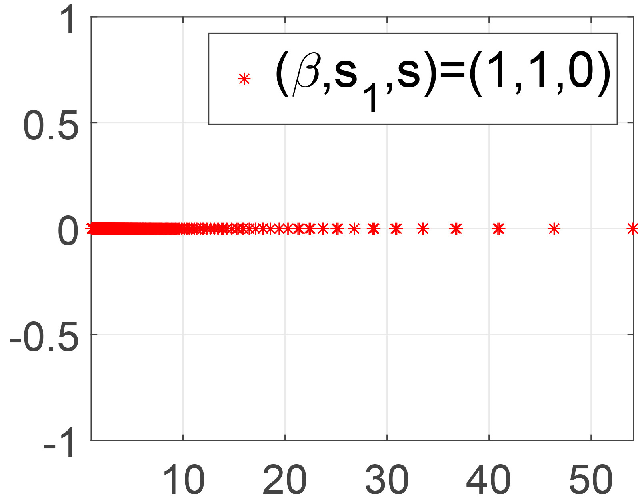
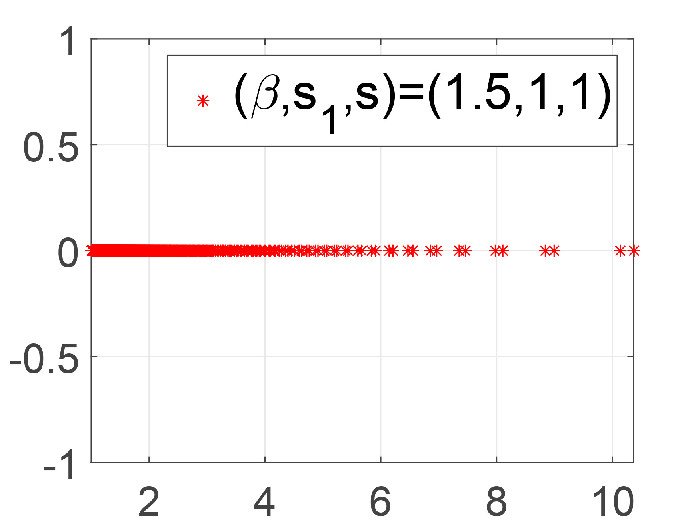
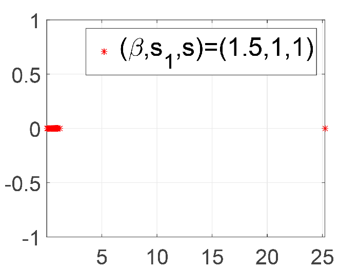
The errors and the corresponding convergence rates with different s,s1,�,�s,s_{1},\beta,\lambda, are listed in Tables 1, which confirm the theoretical analysis in Theorems 2.3 and 3.1. The CUP time and the iterative times of the CG and PCG method are presented in Tables 2 and 3, where “PCG(Ichol)” denotes the perconditioners 𝐁{\bf B} coming from the ichol factorization of the (2​k+1)(2k+1)-bandwidth matrix 𝐆{\bf G} with k=10k=10, and “PCG(T)” denotes that the preconditioner is the T. Chan circulant matrix. The results show that the CPU time spent with PCG methods are much less than those with the Gauss elimination method (the data under “Gauss” in Tables 2 and 3 ) and the CG method, and the T. Chan circulant preconditioner with the iterative times almost independent of hh is a little more effective than the ichol preconditioner. In Figure 1, we display the eigenvalue distribution of the matrix systems with and without preconditioning; after preconditioning, the eigenvalues become clustered around the unity.

Table 1: Errors and convergence rates in Example 4.1 with M=2J−1M=2^{J}-1.
(�,s,s1)(\beta,\,s,\,s_{1}) JJ �=0.5\lambda=0.5 �=3\lambda=3
L2L^{2}-Err Rate L∞L^{\infty}-Err rate L2L^{2}-Err Rate L∞L^{\infty}-Err Rate
1212 2.4068e-06 – 3.7160e-06 – 7.0941e-06 – 1.0474e-05 –
(0.5, 0, 0)(0.5,\,0,\,0) 1313 8.5343e-07 1.50 1.3177e-06 1.50 2.5222e-06 1.49 3.7238e-06 1.49
1414 3.0234e-07 1.50 4.6680e-07 1.50 8.9518e-07 1.49 1.3216e-06 1.49
1212 2.6157e-09 – 4.1651e-09 – 2.7141e-08 – 3.9151e-08 –
(0.5, 1, 1)(0.5,\,1,\,1) 1313 6.5490e-10 2.00 1.0428e-09 2.00 6.8022e-09 2.00 9.8127e-09 2.00
1414 1.6391e-10 2.00 2.6096e-10 2.00 1.7036e-09 2.00 2.4577e-09 2.00
1212 1.3524e-05 – 1.9526e-05 – 6.3501e-05 – 8.6565e-05 –
(1.0, 1, 0)(1.0,\,1,\,0) 1313 6.7700e-06 1.00 9.7756e-06 1.00 3.1824e-05 1.00 4.3391e-05 1.00
1414 3.3872e-06 1.00 4.8911e-06 1.00 1.5932e-05 1.00 2.1725e-05 1.00
1212 1.0989e-08 – 1.6835e-08 – 1.2222e-07 – 1.8135e-07 –
(1.0, 1,1)(1.0,\,1,1) 1313 2.9312e-09 2.02 4.4886e-09 2.02 3.2845e-08 2.01 4.8751e-08 2.01
1414 7.7258e-10 2.03 1.1850e-09 2.02 8.7695e-09 2.01 1.3024e-08 2.01
1212 1.2882e-04 – 1.9477e-04 – 1.8667e-04 – 2.8056e-04 –
(1.5, 1, 0)(1.5,\,1,\,0) 1313 9.1256e-05 0.50 1.3797e-04 0.50 1.3314e-04 0.50 2.0010e-04 0.49
1414 6.4593e-05 0.50 9.7660e-05 0.50 9.4560e-05 0.50 1.4212e-04 0.50
1212 2.4683e-07 – 3.7330e-07 – 2.1634e-06 – 3.2512e-06 –
(1.5, 1, 1)(1.5,\,1,\,1) 1313 8.7460e-08 1.50 1.3226e-07 1.50 7.6763e-07 1.49 1.1536e-06 1.49
1414 3.0694e-08 1.50 4.6482e-08 1.50 2.7217e-07 1.50 4.0906e-07 1.50
Table 2: Performance of the CG and PCG methods in Example 4.1 with �=0.5\lambda=0.5 and M=2J−1M=2^{J}-1.
(�,s,s1)(\beta,\,s,\,s_{1}) JJ CG PCG (Ichol) PCG (T) Gauss
#\# iter CPU(s) #\# iter CPU(s) #\# iter CPU(s) CPU(s)
1212 97 0.8174 40 0.1472 11 0.0182 1.1997
(0.5, 0, 0)(0.5,\,0,\,0) 1313 115 0.3248 44 0.1789 11 0.0627 6.0118
1414 138 2.7400 49 2.1894 11 0.1691 56.6159
1212 74 0.1622 39 0.0851 0 10 0.0159 0.7742
(0.5, 1, 1)(0.5,\,1,\,1) 1313 88 0.3222 43 0.1619 11 0.0609 7.5780
1414 105 3.1492 49 1.1515 11 0.1355 57.7863
1212 329 1.3938 47 0.1632 15 0.0215 0.8483
(1.0, 1, 0)(1.0,\,1,\,0) 1313 468 1.3587 58 0.2424 16 0.0888 6.0763
1414 664 7.3204 71 3.3773 17 0.2877 53.1450
1212 337 0.6903 47 0.7371 15 0.0715 0.8431
(1.0, 1,1)(1.0,\,1,1) 1313 479 1.6629 58 0.2146 16 0.0872 6.1244
1414 680 7.5843 71 3.368 17 0.2486 53.5024
1212 1363 1.8888 30 0.2089 29 0.0356 0.8860
(1.5, 1, 0)(1.5,\,1,\,0) 1313 2300 8.8453 35 0.1220 34 0.1779 6.7129
1414 3880 25.9750 42 0.4814 41 0.4571 55.0814
1212 1383 1.5639 30 0.0609 29 0.0448 0.9285
(1.5, 1, 1)(1.5,\,1,\,1) 1313 2333 7.2669 35 0.1538 33 0.1960- 7.5258
1414 3935 30.7326 42 1.0987 39 0.4440 57.1891
Table 3: Performance of the CG and PCG methods in Example 4.1 with �=3\lambda=3 and M=2J−1M=2^{J}-1.
(�,s,s1)(\beta,\,s,\,s_{1}) JJ CG PCG (Ichol) PCG (T) Gauss
#\# iter CPU(s) #\# iter CPU(s) #\# iter CPU(s) CPU(s)
1212 127 0.2231 70 0.1079 12 0.0207 0.8877
(0.5, 0, 0)(0.5,\,0,\,0) 1313 152 0.5855 88 0.3419 12 0.0544 6.8314
1414 182 5.2566 108 0.9474 12 0.1048 49.5857
1212 97 0.5242 70 0.0897 11 0.0199 0.9509
(0.5, 1, 1)(0.5,\,1,\,1) 1313 116 0.3499 88 0.2889 12 0.0525 6.8463
1414 139 1.7316 107 0.8856 12 0.0989 50.5869
1212 376 0.3920 57 0.0727 17 0.0269 0.8913
(1.0, 1, 0)(1.0,\,1,\,0) 1313 534 1.7202 74 0.3233 17 0.1141 7.2649
1414 758 7.2397 95 3.3281 19 0.2291 57.5678
1212 385 1.1568 57 0.1364 17 0.0610 0.8701
(1.0, 1,1)(1.0,\,1,1) 1313 547 1.8208 75 0.3743 17 0.0991 7.1813
1414 776 12.3254 95 5.1381 19 0.2976 53.7438
1212 1423 1.9613 29 1.8896 30 0.0516 0.8078
(1.5, 1, 0)(1.5,\,1,\,0) 1313 2400 6.6799 35 0.2333 37 0.2130 6.2326
1414 4047 25.8704 42 0.4828 42 0.5635 55.6647
1212 1444 1.3327 29 1.1708 30 0.0382 0.8009
(1.5, 1, 1)(1.5,\,1,\,1) 1313 2435 9.4863 36 0.1528 37 0.1880 6.8698
1414 4104 26.0405 42 0.4805 42 0.5481 51.1018
Refer to caption
Refer to caption
Refer to caption
Refer to caption
Refer to caption
Refer to caption
Refer to caption
Refer to caption
Refer to caption
Figure 1: Eigenvalue distribution of the systems (57) or (92) in Example 4.1 with J=13J=13 and �=3\lambda=3. First column: without preconditioning; second column: preconditioned with the ichol factorization; third column: preconditioned with the T. Chan circulant matrix. The horizontal and vertical axes are respectively the real and imaginary axis.
Example 4.2.

Consider model (1) in =(0,1)\Omega=(0,1) with the boundary condition

g⁡(x)=(−2​x)​�[−12,0]+(2​x−2)​�[1,32]\displaystyle g(x)=(-2x)\chi_{[-\frac{1}{2},0]}+(2x-2)\chi_{[1,\frac{3}{2}]} (131)

and source term f⁡(x)f(x) being derived from the exact solution

p⁡(x)=(−2​x)​�[−12,0]+(x−x2)2​�(0,1)+(2​x−2)​�[1,32].\displaystyle p(x)=(-2x)\chi_{[-\frac{1}{2},0]}+(x-x^{2})^{2}\chi_{(0,1)}+(2x-2)\chi_{[1,\frac{3}{2}]}. (132)

Obviously, u⁡(x)u(x) is discontinuous at x=32x=\frac{3}{2} and x=−12x=-\frac{1}{2}. In the numerical simulation, for �=0\lambda=0, the f⁡(xi),d1​(i),d2​(i)f(x_{i}),\,d_{1}(i),\,d_{2}(i) are obtained exactly; for �≠0\lambda\not=0, they are calculated numerically with the techniques as in Example 4.1. The numerical results are listed in Table 4. Since u⁡(x)u(x) is smooth enough on ¯\bar{\Omega}, the convergence rates are consistent with the theoretical predictions in Theorems 2.3 and 3.1. In fact, for �=0\lambda=0 and �∈(1,2)\beta\in(1,2), the numerical schemes obtained with s1=s=1s_{1}=s=1 seem to have a slightly bigger convergence rate than 3−�3-\beta.

Table 4: Errors and convergence rates in Example 4.2 with M=2JM=2^{J}, solved by the PCG method with T. Chan’s preconditioner.
(�,s,s1)(\beta,\,s,\,s_{1}) JJ �=0\lambda=0 �=3\lambda=3
L2L^{2}-Err Rate L∞L^{\infty}-Err rate iter L2L^{2}-Err Rate L∞L^{\infty}-Err Rate iter
1111 1.1146e-06 – 1.6944e-06 – 8 5.9414e-06 – 9.6168e-06 – 9
(0.5, 0, 0)(0.5,\,0,\,0) 1212 3.9593e-07 1.49 6.0100e-07 1.50 8 2.1173e-06 1.49 3.4273e-06 1.49 9
1313 1.4043e-07 1.50 2.1297e-07 1.50 8 7.5274e-07 1.49 1.2185e-06 1.49 10
1111 4.5687e-09 – 6.7988e-09 – 8 4.8132e-08 – 7.1820e-08 – 9
(0.5, 1, 1)(0.5,\,1,\,1) 1212 1.1421e-09 2,00 1.6999e-09 2.01 8 1.2059e-08 2.00 1.7999e-08 2.00 9
1313 2.8551e-10 2.00 4.2566e-10 2.01 8 3.0193e-09 2.00 4.5084e-09 2.00 9
1111 3.7770e-06 – 6.2802e-06 – 12 4.5179e-05 – 6.3557e-05 – 13
(1.0, 1, 0)(1.0,\,1,\,0) 1212 1.8917e-06 1.00 3.1450e-06 1.00 12 22.2684e-05 0.99 3.1930e-05 0.99 13
1313 9.4664e-07 1.00 1.5737e-06 1.00 13 1.1368e-05 1.00 1.6007e-05 1.00 14
1111 9.4496e-09 – 51.3552e-08 – 12 1.6933e-07 – 2.6506e-07 – 13
1212 2.3615e-09 2.13 3.3872e-09 2.13 12 4.5438e-08 2.02 7.1225e-08 2.02 13
(1.0, 1,1)(1.0,\,1,1) 1313 5.9040e-10 2.12 8.4681e-10 2.12 13 1.2138e-08 2.02 1.9048e-08 2.02 14
1111 5.5961e-05 – 9.0153e-05 – 19 9.7334e-05 – 1.5346e-04 – 20
1212 3.9590e-05 0.50 6.3783e-05 0.50 21 6.9986e-05 0.48 1.1035e-04 0.48 22
(1.5, 1, 0)(1.5,\,1,\,0) 1313 2.8003e-05 0.50 4.5116e-05 0.50 24 4.9910e-05 0.49 7.8692e-05 0.49 25
1010 6.2783e-08 – 8.7275e-08 – 16 — – – – –
1111 1.5532e-08 2.01 2.1605e-08 2.01 19 2.3015e-06 1.49 3.6244e-06 – 20
(1.5, 1, 1)(1.5,\,1,\,1) 1212 3.8558e-09 2.01 5.3661e-09 2.01 21 8.1576e-07 1.50 1.2851e-06 1.50 23
1313 9.5433e-10 2.01 1.3282e-09 2.01 24 2.8888e-07 1.50 4.5524e-07 1.50 25
Example 4.3.

Consider model (1) in =(−r,r)\Omega=(-r,r) with source term f⁡(x)=1f(x)=1 and absorbing boundary condition g⁡(x)=0g(x)=0.

When �=0\lambda=0, the exact solution is [9, Subsection 3.1]

u⁡(x)=�​(r2−x2)�/22�​�​(1+�/2)​�​(1/2+�/2)​for​x∈ .\displaystyle u(x)=\frac{\sqrt{\pi}(r^{2}-x^{2})^{\beta/2}}{2^{\beta}\Gamma(1+\beta/2)\Gamma(1/2+\beta/2)}~~~{\rm for}~x\in\Omega. (133)

It is easy to see that u⁡(x)u(x) has a poor regularity at the boundaries of \Omega. When �≠0\lambda\not=0, u⁡(x)u(x) cannot be obtained explicitly; the errors (i.e., the data under L~2\tilde{L}^{2}-Err and L~∞{\tilde{L}}^{\infty}-Err) under stepsize hh in Table 5 with the L2L^{2} and L∞L^{\infty} norms are, respectively,

‖Uh/2−Uh‖​and​max1≤i≤M​|Uh/2−Uh|,\displaystyle\left\|U_{h/2}-U_{h}\right\|~~{\rm and}~~\max_{1\leq i\leq M}\left|U_{h/2}-U_{h}\right|, (134)

and the convergence rates are measured by using there errors, where h=2​rM+1h=\frac{2r}{M+1} with M=2J−1M=2^{J}-1. The numerical results in Table 5 show that the convergence rates are small for two cases, being consistent with the results in [29, Example 2].

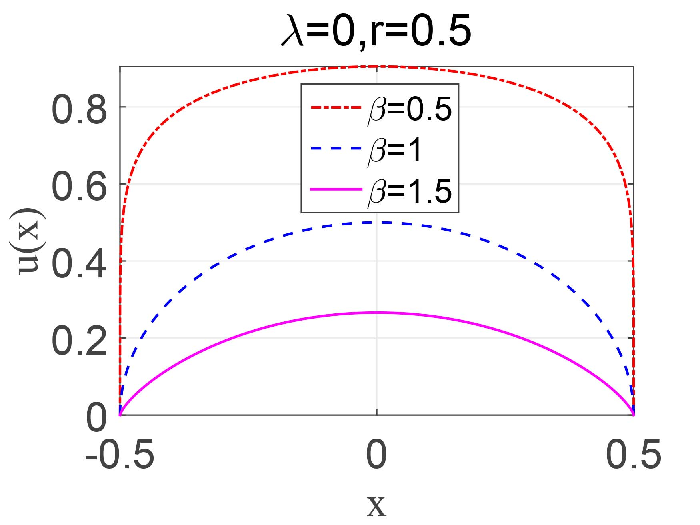
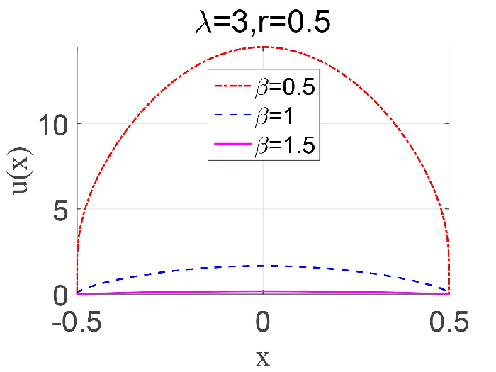
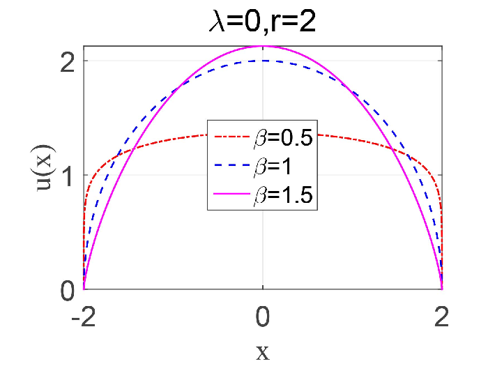
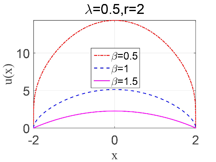
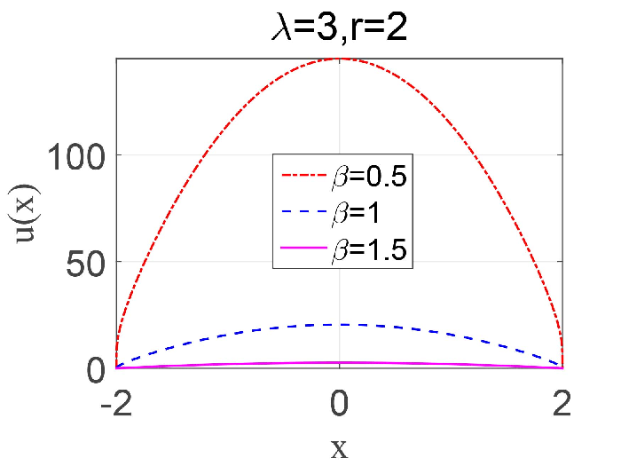
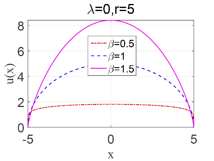
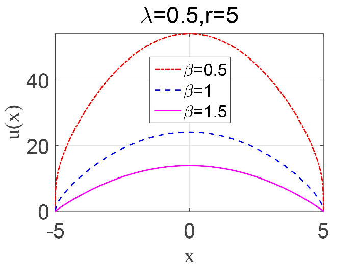
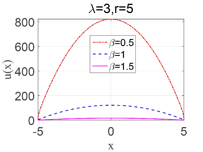
In statistical physics, the solution u⁡(x)u(x) denotes the mean first exit time of a particle starting at xx away from the given domain \Omega [8, 11]. For �=0, 0.5\lambda=0,\,0.5 and 33, the numerical solutions obtained with (s,s1)=(1,1)(s,s_{1})=(1,1) and different values of �=0.5, 1, 1.5,r=1, 2, 5\beta=0.5,\,1,\,1.5,\,r=1,\,2,\,5 are listed in Figures 2, which show: for the same domain \Omega, the mean first exit time increases with the increases of the value of �\lambda; and when �>0\lambda>0, for any fixed value of the starting point xx, the mean exit times are shorter for larger values of �\beta.

Table 5: Errors and convergence rates in Example 4.3 with M=2J−1M=2^{J}-1, solved by the PCG method with T. Chan’s preconditioner. The data in the parentheses denote the rates obtained with the errors in (134).
�=0\lambda=0 �=3\lambda=3
(�,s,s1)(\beta,\,s,\,s_{1}) MM L2L^{2}-Err Rates L∞{L}^{\infty}-Err rates L~2\tilde{L}^{2}-Err Rate L~∞{\tilde{L}}^{\infty}-Err rate
1111 3.5668e-03 – 5.4682e-02 – 3.3886e-02 – 2.2117e-01 –
(0.5, 0, 0)(0.5,\,0,\,0) 1212 2.1205e-03 0.75 (0.75) 4.5975e-02 0.25 (0.25) 1.6834e-02 1.01 1.8113e-01 0.29
1313 1.2608e-03 0.75 (0.75) 3.8658e-02 0.25 (0.25) 8.5734e-03 0.97 1.4951e-01 0.28
1111 1.4675e-03 – 2.0163e-02 – 1.3158e-02 – 8.0461e-02 –
(0.5, 1, 1)(0.5,\,1,\,1) 1212 8.7272e-04 0.75 (0.75) 1.6952e-02 0.25 (0.25) 6.9321e-03 0.92 6.5320e-02 0.30
1313 5.1896e-04 0.75 (0.75) 1.4254e-02 0.25 (0.25) 3.6595e-03 0.92 5.3565e-02 0.29
1111 6.3631e-04 – 4.7004e-03 – 1.6940e-03 – 6.1020e-03 –
(1.0, 1, 0)(1.0,\,1,\,0) 1212 3.3183e-04 0.94 (0.94) 3.3232e-03 0.50 (0.50) 8.7755e-04 0.95 4.2848e-03 0.51
1313 1.7249e-04 0.94 (0.94) 2.3497e-03 0.50 (0.50) 4.4946e-04 0.97 3.0161e-03 0.51
1111 6.3631e-04 – 4.7004e-03 – 1.6940e-03 – 6.1020e-03 –
(1.0, 1, 1)(1.0,\,1,\,1) 1212 3.3183e-04 1.08 (1.08) 3.3232e-03 0.64 (0.64) 8.7755e-04 1.09 4.2848e-03 0.65
1313 1.7249e-04 1.07 (1.07) 2.3497e-03 0.63 (0.63) 4.4946e-04 1.09 3.0161e-03 0.63
1111 1.6135e-03 – 1.3157e-03 – 2.7348e-03 – 2.4835e-03 –
(1.5  1, 0)(1.5\,\,1,\,0) 1212 1.1034e-03 0.55 (0.58) 9.0676e-04 (0.54)  (0.56) 1.9986e-03 0.45 1.8304e-03 0.44
1313 7.6158e-04 0.53 (0.56) 6.2939e-04 (0.53)  (0.54) 1.4278e-03 0.49 1.3146e-03 0.48
1111 2.2426e-04 – 5.4375e-04 – 1.8108e-04 – 5.7640e-04 –
(1.5, 1, 1)(1.5,\,1,\,1) 1212 1.1260e-04 0.99 (0.99) 3.2327e-04 0.75 (0.75) 1.1576e-04 0.65 3.4404e-04 0.74
1313 5.6465e-05 1.00 (1.00) 1.9220e-04 0.75 (0.75) 6.9126e-05 0.74 2.0489e-04 0.75
Refer to caption
Refer to caption
Refer to caption
Refer to caption
Refer to caption
Refer to caption
Refer to caption
Refer to caption
Refer to caption
Figure 2: Dependence of the mean exit time u⁡(x)u(x) on the size of domain \Omega, and the values of �\beta and �\lambda.

5 Conclusion

The tempered fractional Laplacian is a recently introduced operator for treating the weaknesses of the fractional Laplacian in some physical processes. This paper provides several classes of finite difference schemes for the tempered fractional Laplacian equation with �∈(0,2)\beta\in(0,2). According to the regularity of the solution, one can choose the more appropriate numerical schemes. The detailed numerical analyses are performed, and the effective preconditioning techniques are provided. The implementation details are also discussed, including that the entries of the stiffness matrix can be explicitly and conveniently calculated and the stiffness matrix has Toeplitz-like structure. The efficiencies of the algorithms are verified by extensive numerical experiments and the desired convergence rates are confirmed.

Acknowledgments

This work was supported by the National Natural Science Foundation of China under Grant Nos. 11671182 and 11701456, and the Fundamental Research Funds for the Central Universities under Grant No. lzujbky-2017-ot10.

References

  • [1] M. Abramowitz and I. A. Stegun, Handbook of Mathematical Functions, Dover Publications, 1965, Chapter 5.
  • [2] G. Acosta and J. P. Borthagaray, A fractional Laplace equation: regularity of solutions and finite element approximations, SIAM J. Numer. Anal., 55 (2017), pp. 472-495.
  • [3] Advanpix Multiprecision Computing Toolbox for MATLAB, http://www.advanpix.com/, accessed 2017-10-24.
  • [4] D. Applebaum, Lévy Process and Stochastic Calculus, 2nd ed., Cambridge University Press, Cambridge, UK, 2009.
  • [5] O. Axelssion, Iterative Solution Methods, Cambridge University press, UK, 1996.
  • [6] B. Baeumer and M. M. Meerschaert, Tempered stable Lévy motion and transient supper-diffusion, J. Comput. Appl. Math., 233 (2010), pp. 2438-2448.
  • [7] R. H. Chan and X. Q. Jin, An Introduction to Iterative Teoplitz Solvers, SIAM, 2007.
  • [8] W. H. Deng, X. C. Wu, and W. L. Wang, Mean exit time and escape probability for the anomalous processes with the tempered power-law waiting times, EPL, 117 (2016).
  • [9] W. H. Deng, B. Y. Li, W. Y. Tian, and P. W. Zhang, Boundary problems for the fractional and tempered fractional operators, Multiscale Model. Simul., in press, 2017.
  • [10] T. Gao, J. Duan, X. Li, and R. Song, Mean exit time and escape probabilty for dynamical systems driven by Lévy noises, SIAM J. Sci, Comput., 36 (2014), pp. A887-A906.
  • [11] R. K. Getoor, First passage times for symmetric stable processes in space, Trans. Amer. Math. Soc., 101 (1961), pp. 75-90.
  • [12] I. S. Gradshteyn, I. M. Ryzhik, Y. V. Geraniums, and M. Y. Tseytlin, Table of Integrals, Series, and Products, A. Jeffrey, ed., Translated by Scripta Technica, Academic Press, USA, 1980.
  • [13] J. S. Hesthaven and T. Warburton, Nodal Discontinuous Galerkin Methods: Algorithms, Analysis, and Applications, Springer, Berlin, 2008.
  • [14] J. F. Huang, Y. F. Tang, and L. Vázquez, Convergence analysis of a block-by-block method for fractional differential equations, Numer. Math. Theor. Meth. Appl. 5 (2012), pp. 229-241.
  • [15] Y. H. Huang and A. Oberman, Numerical methods for the fractional Laplacian: a finite difference-quadrature approach, SIAM. J. Numer. Anal. 52 (2014), pp. 3056-3084.
  • [16] J. H. Jia and H. Wang, Fast finite difference methods for space-fractional diffusion equations with fractional derivative boundary conditions, J. Comput. Phys., 293 (2015), pp. 359-369.
  • [17] S. L. Lei and H. W. sun, A circulant preconditioner for fractional diffusion equations, J. Comput. Phys., 242 (2013), 715-725.
  • [18] C. Li and W. H. Deng, High order schemes for the tempered fractional diffusion equations, Adv. Comput. Math., 42 (2016), pp. 543–572.
  • [19] F. R. Lin, S. W. Yang, and X. Q. Jin, Preconditioned iterative methods for fractional diffusion equation, J. Comput. Phys., 256 (2014), pp. 109-117.
  • [20] M. M. Meerschaert and C. Tadjeran, Finite difference approximations for fractional advection-dispersion flow equations, J. Comput. Appl. Math., 172 (2004), pp. 65-77.
  • [21] J. Y. Pan, R. Ke, M. K. NG, and H. W. Sun, Precondtioing techniques for diagonal-times-Toeplitz matrices in fractional diffusion equations, SIAM J. Sci. Comput., 36 (2014), pp. A2698-A2719.
  • [22] S. Peszat and J. Zabczyk, Stochastic Partial Differential Equations with Lévy Processes, Cambridge University Press, Cambridge, UK, 2007.
  • [23] C. Pozrikidis, The Fractional Laplacian, CRC Press, London, 2016.
  • [24] F. Sabzikar, M. M. Meerschaert, and J. H. Chen, Tempered fractional calculus, J. Comput. Phys., 293 (2015), pp. 14-28.
  • [25] J. Shen, T. Tang, and L. L, Wang, Spectral Methods: Algorithms, Analysis and Applications, Springer, New York, 2011.
  • [26] C. T. Sheng and J. Shen, A hybrid spectral element method for fractional two-point boundary value problems, Numer. Math. Theor. Meth. Appl. 10 (2017), pp. 437-464.
  • [27] Q. Yang, F. Liu, and I. Turner, Numerical methods for fractional partial differential equations with Riesz space fractional derivatives, Appl. Math. Model., 34 (2010), pp. 200-218.
  • [28] V. Zaburdaev, S. Denisov, and J. Klafter, Lévy walks, Rev. Modern Phys., 87 (2015), pp. 483-530.
  • [29] Z. J. Zhang, W. H. Deng, and G. E. Karniadakis, A Riesz basis Galerkin method for the tempered fractional Laplacian, arXiv:1709.10415, 2017.
  • [30] Z. Zhao, X. Q. Jin, and M. M. Lin, Preconditioned iterative methods for space-time fractional advection-diffusion equations, J. Comput. Phys., 319 (2016), pp. 266-279.
  • [31] X. Zhao, Z. Z. Sun, and Z. H. Hao, A fourth-order compact ADI scheme for two-dimensional nonlinear space fractional Schrödinger equation, SIAM J. Sci. Comput., 36 (2014), pp. A2865-A2886.