Planet-Metallicity Correlation in M-dwarfs \addkeywordMethods: observational \addkeywordTechniques: spectroscopic \addkeywordStars: abundances \addkeywordPlanets and satellites: general
Testing the Planet-Metallicity Correlation in M-dwarfs with Gemini GNIRS Spectra
Abstract
Mientras que la correlación planeta-metalicidad para las estrellas de secuencia principal FGK que albergan planetas gigantes está bien establecida, los resultados no son tan claros para las estrellas enanas M, para las cuales las deteminaciones de metalicidad son complejas. Sin embargo, técnicas nuevas con espectros infrarrojos muestran resultados prometedores. Aplicando estos métodos se determinan parámetros estelares y metalicidades de 16 estrellas enanas M, incluyendo 11 con planetas detectados, a partir de espectros infrarrojos de resolución moderada obtenidos con el instrumento GNIRS (Gemini Near-Infrared Spectrograph) del telescopio Gemini Norte. Se encuentra que las enanas M con planetas son preferentemente ricas en metales en comparación con aquéllas sin planetas. Este resultado, basado en espectros GNIRS, es avalado por el análisis de una muestra relativamente mayor de estrellas M con planetas (18 en total) y una muestra de control de 213 estrellas M sin planetas detectados, obtenidas del catálogo de Terrien et al. (2015). Esto, por un lado, coincide con la tendencia reportada en la literatura (tanto para estrellas M como de masa solar) y, por el otro, demuestra la utilidad de los espectros de GNIRS para la obtención de parámetros estelares confiables de estrellas M. Adicionalmente encontramos que las enanas M que albergan planetas gigantes son preferentemente más metálicas que aquéllas asociadas con planetas de menor masa (de tipo Neptuno o súper-Tierra). Esta tendencia también concuerda con la reportada previamente para estrellas de tipo solar. Estos resultados favorecerían el modelo de acreción del núcleo para la formación planetaria.
0.1 Introduction
M-dwarf stars are the greatest stellar component of the Galaxy, representing around of stars (Kroupa et al., 2013). They are small, cool, faint stars, with masses ranging from to , radii from to , temperatures from K to K, and luminosities from to (Kaltenegger & Traub, 2009). As the greatest stellar population, they may also represent the greatest population of planetary hosts (e.g. Lada 2006).
Nowadays it is widely accepted that FGK main-sequence and subgiant stars hosting gas giant planets are, on average, more metal-rich than stars without detected planets (e.g. Gonzalez 1997, Fischer & Valenti 2005, Ghezzi et al. 2010b). However, the existence of a planet-metallicity correlation is not so clear for stars hosting Neptune-sized and smaller planets (e.g. Sousa et al. 2011, Mayor et al. 2011, Neves et al. 2013, Buchhave & Latham 2015, Wang & Fischer 2015). Moreover, the results for giant stars with planets have been ambiguous, and the issue is still debated (e.g. Maldonado et al. 2013, Jofré et al. 2015, Reffert et al. 2015).
There are two generally accepted models for planetary formation: gravitational instability and core accretion. In the gravitational instability model, dust particles settle into a thin disk with local overdense regions, which are unstable and undergo gravitational collapse. Successive collapses and collisions are responsible for the formation of planets (e.g. Goldreich & Ward 1973, Boss 1997, Youdin & Shu 2002). In the core accretion model, on the other hand, terrestrial planets and the solid cores of gas planets are formed by the accumulation of planetesimals. If a critical mass is reached before gas depletion, gas accretion from the disk begins and forms a giant planet (e.g. Pollack et al. 1996, Mordasini et al. 2009).
The planet-metallicity correlation found for main-sequence FGK stars would provide support for the core accretion planet formation scenario. A more metallic environment allows the rapid formation of planetary cores which can start to accrete gas from the surrounding disk to form gas giant planets (Pollack et al., 1996), whereas in low-metallicity the cores form too slowly for accretion to take place before the disk is depleted (Ida & Lin 2004, Mayor et al. 2011, Mordasini et al. 2012). The considerably low metallicity ([Fe/H] 0.30 dex, e.g. Santos et al. 2010) of several main-sequence (MS) stars hosting giant planets, and the average low metallicity found for giant stars with planets ( 0.08 dex; Jofré et al. 2015) raises the issue of giant planet formation within the framework of the metallicity-dependent core accretion model. Johnson & Li (2012) derived the minimum metallicity function required for planet formation in the core accretion scenario, and found that none of the 320 planet-hosting stars reported by 2011 were below the critical metallicity. Similar results are found for evolved stars with planets (Jofré et al., 2015). On the other hand, it has been suggested that the more massive disks around higher-mass stars, such as evolved stars with planets11 1 Giants with planets usually have masses between 0.9 and 4 (e.g., Sato et al. 2005, Niedzielski et al. 2007, Jofré et al. 2015, Ghezzi & Johnson 2015)., would compensate their lower metallic abundances and hence enable giant-planet formation (Ghezzi et al. 2010a, Maldonado et al. 2013). The situation for the formation of giant planets around M-dwarfs may be even less clear, since theoretical predictions within the core accretion model foresee that the giant-planet-formation may be inhibited at all radial distances (Laughlin et al., 2004).
Given the role that stellar properties, such as metallicity and mass, may play in the process of planet formation, it is also key to confirm (or refute) the planet-metallicity correlation results for stars at the lower end of the mass scale, such as M dwarfs. However, while for FGK stars metallicities can be determined with great accuracy using high-resolution spectra () in the optical range, the spectra of M-dwarf stars are extremely complex, with many blended lines and strong molecular bands (e.g., TiO, VO) preventing an easy continuum fit and thus complicating a precise metallicity determination. While some studies (e.g., Bean et al. 2006, Woolf & Wallerstein 2006) have attempted determinations using high-resolution optical spectra, they have been limited to few and/or metal-poor stars. Önehag et al. (2012) adopted a slightly different approach, using high-resolution spectra () in the infrared J band; this spectral region has few molecular components, enabling precise continuum and line fitting. The need for high resolution, however, limits this technique, as bright stars and/or long integration times are necessary. Additionally, M dwarfs are typically brighter in the H and K bands than in the J band.
Wide-band photometric calibrations using VK and were performed for M-dwarfs by Bonfils et al. (2005a), Johnson & Apps (2009), and Schlaufman & Laughlin (2010), with conflicting results: Johnson & Apps (2009) find that only Jupiter hosts are metal-rich, while Schlaufman & Laughlin (2010) report that both Jupiter and Neptune hosts are metal-rich. For Jupiter hosts, both results are therefore in agreement with that found for FGK stars, whereas the situation for Neptune hosts is not clear for either FGK stars or M-dwarfs. Bonfils et al. (2005a) studied only two planetary hosts, Gl 876 and Gl 436, finding near-solar metallicities for both. Additionally, Schlaufman & Laughlin (2010) note that Bonfils et al. (2005a) systematically underestimate metallicities, while Johnson & Apps (2009) overestimate them. The main disadvantage of these photometric techniques is the need for absolute magnitudes; their determination requires accurate stellar distances, which limits the stars to which these techniques can be applied. However, it is expected that the ongoing ESA astrometric mission, Gaia (Gaia Collaboration et al., 2016) provides accurate distances for all objects down to G 20 mag 22 2 G represents the broad-band, white-light, Gaia magnitude with wavelength coverage 330-1050 nm., and therefore the number of M stars whose metallicities could be determined by the photometric techniques would be significantly increased.
Recently, a new technique for determining the metallicities of M dwarfs via near infrared (nIR) spectra was developed by Rojas-Ayala et al. (2010) and Terrien et al. (2012). This technique requires only moderate-resolution nIR spectra to reliably estimate metallicities, which greatly reduces the observing time required. Additionally, it is not limited to nearby stars with known parallaxes. It is calibrated using wide FGK-M binaries: assuming a common origin, and therefore a common metallicity, for both stars, the metallicity of the FGK component is measured using high-resolution spectroscopy and assigned to the M-dwarf companion. Linear regressions are then performed between these metallicities and the equivalent widths (EWs) of the selected nIR spectral features, resulting in a best-fit relationship between the EWs and the metallicity. Using this technique, Rojas-Ayala et al. (2012) find an apparent planet-metallicity correlation over 133 M dwarfs including 11 planet hosts, which is strongest for Hot Jupiters, using spectra from the TripleSpec spectrograph on the Palomar 200-inch Hale Telescope with . Likewise, Terrien et al. (2012) find that five giant planet hosts are more metal-rich than four M-dwarf planet hosts without known giant planets, using spectra from the NASA-Infrared Telescope Facility SpeX Spectrograph with 33 3 We note that H- and/or K-band spectra have not only been applied to derive metallicities of M dwarfs with planets, but also of late-type stars in the Kepler field (Muirhead et al., 2014), of nearby M-dwarfs (Newton et al., 2014) and of mid- and late-M dwarfs (Mann et al., 2015), in general..
Gaidos & Mann (2014) used JHK spectra to derive metallicities of 121 M dwarfs and study the occurrence of giant planets with metallicity for both M-dwarfs and solar-type stars. Their results hint to a deficiency of giant planets in M dwarfs, although this deficiency is not very significant. More recently, Gaidos et al. (2016), using a photometric calibration in JH, obtained metallicities for M dwarfs and found that the distribution in metallicity of M dwarfs with planets (usually small planets) is indistinguishable from that of M dwarfs without known planets. Souto et al. (2017), using high-resolution (R 22,500) H-band spectra from the SDSS-IV-APOGEE survey, derived chemical abundances for 13 elements for two M-dwarfs with multiplanetary systems, Kepler 138 and Kepler 186, and obtained sub-solar metallicities. They found, however, that in both cases previous metallicity determinations from lower-resolution spectra were sub-estimated by 0.1– 0.2 dex.
Taking into account the lack of consensus about the planet-metallicity correlation in M dwarf stars, in this work we applied the techniques developed in the nIR to homogeneously determine stellar parameters and metallicities of 16 M dwarfs (11 of which have planets) from spectra obtained with the Gemini North Near-Infrared Spectrograph (GNIRS). In § 0.2 we present the observations and data reduction; in § 0.3 the determinations of the stellar parameters, including metallicity; searches for correlations between metallicity and planetary parameters are presented in § 0.4. To test if trends suggested by GNIRS spectra are also supported by relatively larger samples, we used two subsamples of M dwarfs with and without known planets from the catalogue of Terrien et al. (2015). Finally in § 0.5 we summarize the conclusions.
0.2 Observations and Data Reduction
NIR spectra were obtained for a sample of 11 M dwarfs with planets and 5 without known planets using the GNIRS spectrograph, mounted on the Gemini North telescope. The observations were carried out during the 2012B and 2013A semesters (programs GN-2012B-Q-23 and GN-2013A-Q-66 respectively). In the 2012B program, five stars were observed: GJ 176, GJ 179, GJ 250 B, GJ 297.2 B, and GJ 317. The remaining 11 stars (GJ 436, GJ 581, GJ 611 B, GJ 649, GJ 777 B, GJ 783.2 B, GJ 849, GJ 876, GJ 1214, HIP 57050, and HIP 79431) were observed in the 2013A program. The spectrograph was used in cross-dispersed mode, covering a range of , with ; to achieve this, the 10.5 l/mm grating, long blue camera (0.05 arcsec/pix) plus the SXD prism and a 0.45 arcsec slit were employed. Table 1 lists the M-stars observed, the V and K magnitudes, the corresponding telluric standard stars, and the number of planets and discovery papers where applicable.
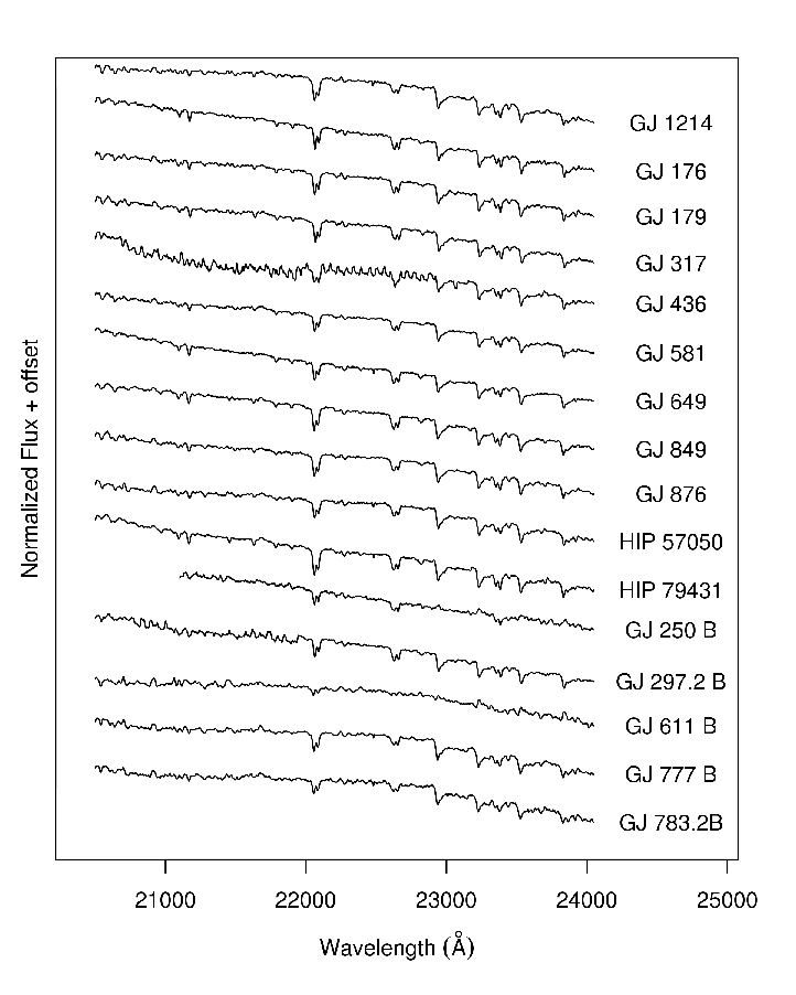
The spectra were reduced using the XDGNIRS pipeline developed by Rachel Mason and Omaira González-Martín44 4 Obtained from http://drforum.gemini.edu/wp-content/uploads/2013/11/XDGNIRS_v20.pdf. This pipeline creates and subtracts the flatfield, removes electronic pattern noise, cuts and straightens the orders, wavelength calibrates, extracts the spectrum, removes telluric lines (based on a telluric standard, listed in Table 1 for each star), flux calibrates, and calculates the SNR of the spectrum. Finally, the reduced spectra were normalised using standard IRAF55 5 IRAF is distributed by the National Optical Astronomy Observatories, which are operated by the Association of Universities for Research in Astronomy, Inc., under cooperative agreement with the National Science Foundation. tasks. The Signal-to-Noise Ratio (SNR) in the observed spectra for the region (calculated as mean/rms of the normalised spectra in the region) are listed in Table 1. Figures 1 and 2 show the normalised spectra in the H and K bands respectively. The targets in our sample have radial velocities 100 kms-1, so any spectral-feature-wavelength displacement would be 10-3 m, and thus indistinguishable within our resolution.
6
| Star | V\tabnotemark | K\tabnotemark | SNR\tabnotemark | Telluric Standard | Planets | Reference |
| GJ 1214 | 14.67 | 8.782 | 101 | HIP 87108 | 1 | 1 |
| GJ 176 | 9.951 | 5.607 | 85 | HIP 22913 | 1 | 2 |
| GJ 179 | 12.018 | 6.942 | 95 | HIP 22913 | 1 | 3 |
| GJ 317 | 11.975 | 7.028 | 83 | HIP 43269 | 2 | 4 |
| GJ 436 | 10.613 | 6.073 | 40 | HIP 57014 | 1 | 5 |
| GJ 581 | 10.560 | 5.837 | 91 | HIP 73249 | 3 | 6, 7, 8 |
| GJ 649 | 9.655 | 5.624 | 86 | HIP 85790 | 2 | 9, 10 |
| GJ 849 | 10.366 | 5.594 | 86 | HIP 109442 | 2 | 11, 12 |
| GJ 876 | 10.192 | 5.010 | 96 | HIP 115119 | 4 | 13, 14, 15, 16 |
| HIP 57050 | 11.959 | 6.822 | 82 | HIP 57014 | 1 | 17 |
| HIP 79431 | 11.372 | 6.589 | 64 | HIP 79124 | 1 | 18 |
| Star | V\tabnotemark | K\tabnotemark | SNR\tabnotemark | Telluric Standard | ||
| GJ 250 B | 10.05 | 5.72 | 42 | HIP 33420 | ||
| GJ 297.2 B | 11.815 | 7.418 | 52 | HIP 42444 | ||
| GJ 611 B | 14.206 | 9.159 | 82 | HIP 78649 | ||
| GJ 777 B | 14.40 | 8.712 | 76 | HIP 98699 | ||
| GJ 783.2 B | 13.932 | 8.883 | 67 | HIP 99742 | ||
| \tabnotetext Obtained from SIMBAD, http://simbad.u-strasbg.fr/simbad/ (Wenger et al., 2000). \tabnotetextSNR for the region. \tabnotetextReferences: (1) Charbonneau et al. (2009); (2) Endl et al. (2008); (3) Howard et al. (2010); (4) Johnson et al. (2007); (5) Butler et al. (2004); (6) Bonfils et al. (2005b); (7) Udry et al. (2007); (8) Mayor et al. (2009); (9) Johnson et al. (2010); (10) Wittenmyer et al. (2013); (11) Butler et al. (2006); (12) Montet et al. (2014); (13) Delfosse et al. (1998); (14) Marcy et al. (2001); (15) Rivera et al. (2005); (16) Rivera et al. (2010); (17) Haghighipour et al. (2010); (18) Apps et al. (2010). |

0.3 Analysis
0.3.1 Fundamental Stellar Parameters
In this section we use our GNIRS/Gemini spectra and the calibrations from Newton et al. (2015) to calculate temperatures, radii, and Log L of the stars in our sample and compare them with previous estimations from the literature. The aim is to verify whether GNIRS/Gemini spectra are suitable to derive fundamental stellar parameters.
Calibrations from Newton et al. (2015) make use of the equivalent widths (EWs) of the Al doublet at and three Mg lines at , , and in the H band. For details about the precise feature windows and regions used to estimate the continuum for each line, we refer the reader to Table 1 of Newton et al. (2015). The EWs66 6 For all EWs measured in this work, we visually verified that spectral features were included in the defined windows in spite of any (modest) shifts due to stellar radial velocities. were calculated from the standard definition:
| (1) |
with the pixels spanned by the line, the wavelength at pixel , the observed line intensity at pixel , the calculated continuum intensity at pixel , and the pixel width. The continuum for each line was defined, in accordance with Newton et al. (2015), as a linear fit to the corresponding blue and red continuum regions. Once the EWs were measured, we calculated the stellar parameters using the expresions:
| (2) |
| (3) |
| (4) |
with the equivalent width measured for element X.
The results are reported in Table 2. The errors were estimated using Monte Carlo methods: random Gaussian noise based on the SNR was added to each spectrum, and the EWs were recalculated. We performed this 100 times for each target, and estimated the EW errors as the standard deviation of the 100 runs. The errors of the parameters were then obtained by propagation in quadrature. All the stellar parameters of GJ 611 B and GJ 1214 were outside the ranges in which Newton et al. (2015)’s calibrations are valid, so those objects were omitted from the table. Additionally, for other stars only some of the parameters were outside these ranges; for these stars, we report only the parameters with the ranges of validity.
For the temperatures we found average differences of 13, 34, and 20 K with the estimations from Mann et al. (2013), Terrien et al. (2015), and Newton et al. (2015), respectively. These differences are within the uncertainties of our temperatures. With Rojas-Ayala et al. (2012) we found an average difference of 100 K. We point out that this comparison is only possible for 8 and 5 stars in the case of Mann et al. (2013) and Newton et al. (2015), respectively. With regard to Rojas-Ayala et al. (2012) and Terrien et al. (2015) we have 11 stars in common for which temperatures are provided.
The comparison of radii and luminosities is rather limited due to the small number of objects. However, for the 5 stars (GJ 176, GJ 436, GJ 581, GJ 649, and GJ 876) we have in common with Newton et al. (2015), we found a reasonably good agreement with an average difference of 0.05 R⊙, which is of the same order as the errors in our determinations. A similar result was found for Log L with an average difference of 0.1 L⊙. Terrien et al. (2015) provide radii for 13 stars in common with our sample. Our determinations agree with thier published values, with an average difference of 0.02 R⊙. Unfortunaltely, no individual values of radius and luminosity are reported in the other works cited above.
To explore the existence of any systematic difference that might be masked in the determination of the final values of temperatures, radii and luminosities, we directly compared our measured EWs for Al-a, Al-b, Mg(), Mg(), and Mg() with those from the literature. As mentioned above we have only 5 stars in common with Newton et al. (2015) which prevents a detailed analysis, and 16 stars with Terrien et al. (2015). However, we found a good agreement in both cases, suggesting an absence of systematic differences in the EWs measured from GNIRS spectra with respect to previous determinations. A more thorough comparison to definitely rule out any difference would require a larger common sample.
5
| Star | Temperature [K] | Radius [] | Log L [] |
|---|---|---|---|
| GJ 176 | |||
| GJ 179 | |||
| GJ 250 B | \tabnotemark | \tabnotemark | |
| GJ 297.2 B | |||
| GJ 317 | |||
| GJ 436 | |||
| GJ 581 | |||
| GJ 649 | |||
| GJ 777 B | \tabnotemark | \tabnotemark | |
| GJ 783.2 B | \tabnotemark | \tabnotemark | |
| GJ 849 | |||
| GJ 876 | |||
| HIP 57050 | |||
| HIP 79431 | |||
| \tabnotetextParameter outside the ranges in which Newton et al. (2015)’s calibrations are valid. |
0.3.2 Stellar Metallicities
To estimate the stellar metallicities, we used the calibrations developed by Rojas-Ayala et al. (2010), which were updated in Rojas-Ayala et al. (2012), those determined by Terrien et al. (2012), and those developed by Mann et al. (2013). While all these calibrations are based on moderate-resolution nIR spectra, there are differences between them: Rojas-Ayala et al. (2012) only use lines from the K-band - Na I doublet ( and ) and Ca I triplet (, , and ) - and define the continuum via linear fits to regions close to each line. Terrien et al. (2012) give calibrations for both the K-band - Na () and Ca () lines - and the H band - Ca ( and ) and K () lines, and define a continuum for the whole of each band using fourth-order Legendre polynomials. Finally, Mann et al. (2013) select regions empirically determined to be sensitive to metallicity changes in the H, J, and K bands, and define the continuum by linear fits over regions close to each line. The precise feature windows for each line and the regions used to define the continuum can be consulted in the corresponding works. As an example, Figure 3 shows the spectral lines employed for each calibration and the regions used to define the continuums for GJ 1214.
For all calibrations, the EWs were calculated by definition using Eq. 1. The fourth-order Legendre polynomial continuum fits for Terrien et al. (2012)’s calibration were performed using the IRAF splot task, whereas the linear continuum fits for Rojas-Ayala et al. (2012)’s and Mann et al. (2013)’s calibrations were carried out with least-square regression methods.
In addition to the EWs of the spectral lines, all calibrations also use indices in their metallicity determinations to account for the effects of stellar temperature. These indices are given by:
| (5) |
(Rojas-Ayala et al., 2012) and
| (6) |
(Terrien et al., 2012), with the mean flux in the range defined by and (in ). Mann et al. (2013) employed Terrien et al. (2012)’s H-band index and Rojas-Ayala et al. (2012)’s K-band index. The final calibration equations are:
| (7) |
| (8) |
(Terrien et al., 2012), and
| (9) |
Table 3 presents the metallicities obtained by each method. Both the errors of the EWs, and the quoted uncertainties of the calibrations employed, are sources of uncertainty in the metallicity determinations. Taking a conservative approach, we chose to adopt for the metallicity error the largest value between that obtained by propagating the EWs and indices errors, and the quoted uncertainty of the calibration employed (0.14 for Rojas-Ayala et al. 2012, 0.12 for Terrien et al. 2012, 0.07 for Mann et al. 2013 in the H band, and 0.06 for Mann et al. 2013 in the K band), in each case.
The errors for the EWs and indices required by Rojas-Ayala et al. (2012)’s and Mann et al. (2013)’s calibrations were estimated using Monte Carlo methods: random Gaussian noise based on the SNR was added to each spectrum, and the EWs and indices were recalculated. We performed this 1000 times for each target, and estimated the EWs and indices errors as the standard deviation of the 1000 runs. For Terrien et al. (2012)’s calibration, the more elaborate continuum fit made Monte Carlo error estimations too complex. Therefore, we used an analytic method developed by Sembach & Savage (1992), which was also employed by Terrien et al. (2012). Two stars in Table 3, GJ 250 B and GJ 611 B, show different metallicity values depending on calibrations or spectral bands used. Our spectrum for GJ 250 B has relatively lower SNR in comparison with the rest of the stars in Table 3 (see Table 1). In the case of GJ 611 B, it was not possible to achive completely satisfactory telluric correction, resulting in a relatively noisy spectrum. These facts may explain the differences shown in Table 3.
The calibrations of Rojas-Ayala et al. (2012) and Terrien et al. (2012) are based on 20 wide binary stars and are valid for M0–M4 dwarfs and near solar metallicities (0.4 [Fe/H] 0.3). Using a larger number of calibrators (110 wide binaries), Mann et al. (2013) refined these calibrations and expanded the limits of validity in metallicity (1.04 [Fe/H] 0.56) and ranges of spectral types (K5–M6). For all bands, including J-band, Mann et al. (2013) found it possible to obtain reliable metallicities (0.10 dex), although features in the K-band provide the best results.
Recently, Terrien et al. (2015) applied the calibrations of Mann et al. (2013) to a large sample of M dwarfs and compared the results with the ones obtained from other similar calibrations such as the ones of Terrien et al. (2012), Mann et al. (2014), and Newton et al. (2014), all of which were developed with data from the same instrument (IRTF-SpeX, R2000). Finally, they choose the K-band-calibration derived metallicities of Mann et al. (2013) as the preferred measure of [Fe/H] for M1–M5 dwarfs. This calibration is not only based on a larger number of calibrators and has a wider spectral range of validity, but also provides a better agreement with other literature measurements and stability against small radial velocity shifts.

6
| Star | |||||
|---|---|---|---|---|---|
| GJ 176 | |||||
| GJ 179 | |||||
| GJ 250 B | |||||
| GJ 297.2 B | |||||
| GJ 317 | |||||
| GJ 436 | |||||
| GJ 581 | |||||
| GJ 611 B | \tabnotemark | \tabnotemark | |||
| GJ 649 | |||||
| GJ 777 B | |||||
| GJ 783.2 B | |||||
| GJ 849 | |||||
| GJ 876 | |||||
| GJ 1214 | |||||
| HIP 57050 | |||||
| HIP 79431 | |||||
| \tabnotetext1Metallicities obtained following Rojas-Ayala et al. (2012). \tabnotetext2Metallicities obtained following Terrien et al. (2012) for the K band. \tabnotetext3Metallicities obtained following Terrien et al. (2012) for the H band. \tabnotetext4Metallicities obtained following Mann et al. (2013) for the K band. \tabnotetext5Metallicities obtained following Mann et al. (2013) for the H band. \tabnotetextTerrien et al. (2012)’s methods could not be applied to this star because the spectra was too noisy to allow for the fitting of the Legendre polynomial continuums. |
0.3.3 Comparison with the literature and selected calibration
In order to check the consistency of our results with previous estimations, we compared the [Fe/H] of the stars we have in common with Rojas-Ayala et al. (2012), Terrien et al. (2012), and Terrien et al. (2015). Unfortunately, Mann et al. (2013) do not provide metallicities with their calibrations. Figure 4 shows the comparison of our [Fe/H] values based on K-band calibrations to those from Rojas-Ayala et al. (2012), Terrien et al. (2012), and Terrien et al. (2015), along with the median offset (77 7 With defined as the median difference between our determinations and the literature values.) and the standard deviation () of the differences. We found that our estimated [Fe/H] are, in general, smaller than the [Fe/H] listed by Rojas-Ayala et al. (2012). On the other hand, our measured [Fe/H] show very good agreement with those derived by Terrien et al. (2012). In the case of the comparison with Terrien et al. (2015), there are two stars (GJ 250 B and GJ 611 B) for which the [Fe/H] we measure deviate considerably and systematically from the values obtained by these authors. As noted in section 0.3.2 this may be attributed to the relatively low quality of our spectra for these stars.
Analogously, Figure 5 shows the comparison of our [Fe/H] values based on H-band calibrations with those from Terrien et al. (2012) and Terrien et al. (2015). Our measured [Fe/H] values are consistent with those of Terrien et al. (2012) within error bars, with exception of GJ 436, for which our spectra has relatively low SNR (see Table 1). Our determinations are in general 0.16 dex lower than those presented by Terrien et al. (2015). In both cases, as has been previously reported by Mann et al. (2013) and Terrien et al. (2015), it can be seen that the results using H-band calibrations show significantly larger scatter than the ones obtained from K-band calibrations.
We also compared EWs and H2O indices when possible. For Rojas-Ayala et al. (2012) we found that our EWs for Na and Ca are, in general, smaller for 13 stars. The average difference is of 10 %. For Terrien et al. (2012) the comparison for 4 stars (GJ 250 B, GJ 297.2 B, GJ 777 B, and GJ 783.2 B) shows a better agreement with our measured EWs with an average difference of 5 %. No equivalent widths are given in Terrien et al. (2015). Comparisons of H2O indices were possible only with those of Rojas-Ayala et al. (2012). In general, our calculated H2O indices are larger than those reported by Rojas-Ayala et al. (2012) with an average difference of 8 %. Larger water indices and smaller EWs are consistent with our [Fe/H] being smaller than those reported by Rojas-Ayala et al. (2012).
Although the spectral types of our stars fall within the range of the calibrations of Rojas-Ayala et al. (2012) and Terrien et al. (2012) (see section 0.3.2) there is one star (HIP 79431) with [Fe/H] value outside the validity range of these two calibrations. In addition three others (GJ 179, GJ 436, and GJ 783.2 B) lie very close to the limits. Moreover, considering the results of Mann et al. (2013) and Terrien et al. (2015), the good agreement between our [Fe/H] and those of Terrien et al. (2015) based on the K-band calibration of Mann et al. (2013), and that our spectra have similar resolution (R1700) to those used to built the Mann et al. (2013) calibrations, the following analyses are based exclusively on the K-band calibration of Mann et al. (2013).


0.4 Planet-metallicity correlation
0.4.1 [Fe/H] for M dwarfs with and without planets
As noted in § 0.1, the existence of a planet-metallicity correlation for M dwarfs has been strongly debated. In this section, we use the metallicities obtained from GNIRS data and the K-band calibration of Mann et al. (2013) to analyze the [Fe/H] of M stars with a without planets. Then, using relatively large and homogeneous samples from Terrien et al. (2015), we perform a similar analysis to verify that the trend found from our sample of 16 M-dwarf stars is consistent with the behaviour of larger samples.
Figure 6 shows the [Fe/H] distributions of our sample of stars with planets (SWP, N11, red continuous line) and without planets (SWOP, N5, black dash-line). The corresponding medians are: 0.25 and 0.25, respectively. The distributions are significantly different, according to the Kolmogorov-Smirnov (K-S, p-value 0.05) test. This result suggests that M-dwarfs with planets are, on average, more metallic than those without planets. Table 4 summarizes the statistics.
6
| Sample | Number | Average | Median | p-value (K-S)\tabnotemark3 |
| ID\tabnotemark1 | of stars | [Fe/H]\tabnotemark2 | [Fe/H]\tabnotemark2 | |
| SWP | 11 | 0.21 | 0.25 | 0.01 |
| SWOP | 5 | 0.44 | 0.25 | |
| \tabnotetext1Notation: SWP: M dwarfs hosting planet/s; SWOP: M dwarfs without detected planet (see text for more details). \tabnotetext2Based on [Fe/H] values derived using GNIRS spectra and the K-band calibration of Mann et al. (2013). \tabnotetext3Probability of being drawn from the same distribution as the control sample, according to the two-sided Kolmogorov-Smirnov (K-S) test. |

To test if the trend found from GNIRS spectra is supported by a larger sample, we used the catalogue of Terrien et al. (2015) that provides homogeneous [Fe/H] values for 886 M dwarfs, based on the K-band calibration of Mann et al. (2013). These authors flagged 16 planet hosts in their sample. We identified two additional stars with planets: GJ 176 (Forveille et al., 2009) and GJ 3323 (Astudillo-Defru et al., 2017). The 18 M dwarfs with planets along with their [Fe/H] values are listed in Table 5.
3
| Name | [Fe/H] | Planet type\tabnotemark |
|---|---|---|
| GJ 1214 | 0.40 | super-Earth |
| GJ 176 | 0.23 | super-Earth |
| GJ 179 | 0.25 | Jupiter |
| GJ 317 | 0.43 | 2 Jupiters |
| GJ 436 | 0.00 | Neptune |
| GJ 581 | 0.02 | Neptune 2 super-Earths |
| GJ 649 | 0.04 | Jupiter super-Earth |
| GJ 849 | 0.50 | 2 Jupiters |
| GJ 876 | 0.31 | 2 Jupiters Neptune super-Earth |
| HIP 57050 | 0.04 | Jupiter |
| HIP 79431 | 0.78 | Jupiter |
| WASP 43 | 0.40 | Jupiter |
| GJ 433 | 0.03 | Jupiter super-Earth |
| WASP 80 | 0.13 | Jupiter |
| GJ 15 A | 0.28 | super-Earth |
| GJ 3323 | 0.06 | 2 super-Earths |
| GJ 3470 | 0.27 | Neptune |
| Kepler 138 | 0.21 | 2 Earths Mars |
| \tabnotetextClassification derived from masses (and/or radii) reported in The Extrasolar Planets Encyclopaedia (available at www.exoplanet.eu). |
To construct a control sample of stars with no evidence of planetary companions, we cross-matched the remaining stars in Terrien et al. (2015) against samples of M dwarfs monitored with the HIRES (Rauscher & Marcy, 2006) and HARPS (Bonfils et al., 2013) spectrographs, and selected all the stars without reported planets. In addition, we also included M dwarfs from the Terrien et al. (2015)’s catalogue with enough photometric measurements (usually more than 6500 data points) obtained with the Kepler space mission and/or the SuperWASP ground-based survey and with no detected planets. In this way, we built a final control sample of 213 M dwarfs that were searched for planets, but for which no planet has been reported so far. The selected M dwarfs without known planets along with the [Fe/H] values from Terrien et al. (2015)’s catalogue are listed in Table 6. We caution, however, that this comparison sample might still include stars hosting low mass and/or long period planets that could be harder to detect by the mentioned surveys.
| Star | [Fe/H] | Star | [Fe/H] |
| 2MASSJ023615350652191 | 0.29 | 2MASSJ122411212653166 | 0.13 |
| 2MASSJ031322990446293 | 0.24 | 2MASSJ234658002750066 | 0.12 |
| 2MASSJ044255811857285 | 0.23 | 2MASSJ122140702707510 | 0.1 0 |
| 2MASSJ050157460656459 | 0.06 | 2MASSJ234614052826036 | 0.05 |
| 2MASSJ065218040511241 | 0.09 | 2MASSJ005801153919111 | 0.03 |
| 2MASSJ101217680344441 | 0.17 | 2MASSJ002706734941531 | 0.25 |
| 2MASSJ102855550050275 | 0.19 | 2MASSJ093014452630250 | 0.22 |
| 2MASSJ105052010648292 | 0.29 | 2MASSJ025641223522346 | 0.24 |
| 2MASSJ114744400048164 | 0.08 | 2MASSJ012700423351580 | 0.33 |
| 2MASSJ132959791022376 | 0.12 | 2MASSJ133451473746195 | 0.21 |
| 2MASSJ143416831231106 | 0.42 | 2MASSJ043100013647548 | 0.12 |
| 2MASSJ151926890743200 | 0.02 | 2MASSJ155121792931062 | 0.11 |
| 2MASSJ175748490441405 | 0.41 | 2MASSJ033023313440325 | 0.09 |
| 2MASSJ180507550301523 | 0.26 | 2MASSJ210124812043377 | 0.15 |
| 2MASSJ184244981354168 | 0.14 | 2MASSJ123628703512007 | 0.10 |
| 2MASSJ190950981740074 | 0.07 | 2MASSJ154938333448555 | 0.34 |
| 2MASSJ192202060702310 | 0.28 | 2MASSJ025916703146245 | 0.01 |
| 2MASSJ204033641529572 | 0.33 | 2MASSJ202605285834224 | 0.30 |
| 2MASSJ220940290438267 | 0.50 | 2MASSJ121302912146388 | 0.35 |
| 2MASSJ225316721415489 | 0.31 | 2MASSJ160613632901553 | 0.51 |
| 2MASSJ225634971633130 | 0.37 | 2MASSJ234353103235388 | 0.03 |
| 2MASSJ001825494401376 | 0.1 | 2MASSJ173736482205510 | 0.08 |
| 2MASSJ020012781303112 | 0.15 | 2MASSJ033608683118398 | 0.04 |
| 2MASSJ023615350652191 | 0.29 | 2MASSJ103617942844471 | 0.18 |
| 2MASSJ065218040511241 | 0.09 | 2MASSJ234420842136050 | 0.28 |
| 2MASSJ085240842818589 | 0.49 | 2MASSJ020002804345286 | 0.09 |
| 2MASSJ101217680344441 | 0.17 | 2MASSJ103508593349499 | 0.04 |
| 2MASSJ102855550050275 | 0.19 | 2MASSJ020002804345286 | 0.09 |
| 2MASSJ105052010648292 | 0.29 | 2MASSJ233855682101218 | 0.11 |
| 2MASSJ114744400048164 | 0.08 | 2MASSJ230715242307533 | 0.06 |
| 2MASSJ132959791022376 | 0.12 | 2MASSJ222250802801475 | 0.22 |
| 2MASSJ143416831231106 | 0.42 | 2MASSJ021320623648506 | 0.05 |
| 2MASSJ175748490441405 | 0.41 | 2MASSJ153837083707247 | 0.01 |
| 2MASSJ180507550301523 | 0.26 | 2MASSJ112637573756237 | 0.15 |
| 2MASSJ183436644007266 | 0.84 | 2MASSJ035643303254082 | 0.07 |
| 2MASSJ224649804420030 | 0.05 | 2MASSJ185626284622532 | 0.01 |
| 2MASSJ225634971633130 | 0.37 | 2MASSJ033235782843554 | 0.19 |
| 2MASSJ234154984410407 | 0.55 | 2MASSJ134555272723131 | 0.18 |
| 2MASSJ185504514259510 | 0.11 | 2MASSJ033235782843554 | 0.19 |
| 2MASSJ190513353845050 | 0.06 | 2MASSJ234508683003184 | 0.15 |
| 2MASSJ190517394507161 | 0.19 | 2MASSJ185233734538317 | 0.04 |
| 2MASSJ191705584007235 | 0.19 | 2MASSJ112816253136017 | 0.20 |
| 2MASSJ192421004237254 | 0.44 | 2MASSJ135149384157445 | 0.39 |
| 2MASSJ192717534231537 | 0.07 | 2MASSJ135051813644168 | 0.07 |
| 2MASSJ195109304628598 | 0.05 | 2MASSJ113531983855372 | 0.08 |
| 2MASSJ172830393727074 | 0.09 | 2MASSJ122426652545077 | 0.06 |
| 2MASSJ170740354918351 | 0.01 | 2MASSJ160413222331386 | 0.13 |
| 2MASSJ173405624447082 | 0.23 | 2MASSJ112404343808108 | 0.00 |
| 2MASSJ173634854549324 | 0.40 | 2MASSJ022240823055161 | 0.03 |
| 2MASSJ163527403500577 | 0.06 | 2MASSJ103313673409120 | 0.15 |
| 2MASSJ173026723344522 | 0.26 | 2MASSJ221821354356406 | 0.15 |
| 2MASSJ171738575224227 | 0.01 | 2MASSJ014016493147306 | 0.25 |
| 2MASSJ170323845124219 | 0.03 | 2MASSJ103359712922465 | 0.03 |
| 2MASSJ164544103605496 | 0.22 | 2MASSJ002520632253121 | 0.01 |
| 2MASSJ170926013909384 | 0.2 | 2MASSJ002434783002295 | 0.23 |
| 2MASSJ170807104829268 | 0.02 | 2MASSJ213954332736439 | 0.25 |
| 2MASSJ170726703900429 | 0.11 | 2MASSJ205920355303049 | 0.13 |
| 2MASSJ171011014139340 | 0.11 | 2MASSJ171959482412054 | 0.10 |
| 2MASSJ232258353717143 | 0.10 | 2MASSJ171905772253036 | 0.35 |
| 2MASSJ171011014139340 | 0.11 | 2MASSJ002853915022330 | 0.15 |
| 2MASSJ222948854128479 | 0.02 | 2MASSJ130934952859065 | 0.02 |
| 2MASSJ164950344745402 | 0.16 | 2MASSJ050305632122362 | 0.07 |
| 2MASSJ164804544522429 | 0.09 | 2MASSJ124626722626368 | 0.08 |
| 2MASSJ153154272851096 | 0.19 | 2MASSJ125034572655230 | 0.1 |
| 2MASSJ165339155603272 | 0.22 | 2MASSJ043422484302148 | 0.22 |
| 2MASSJ163128064710212 | 0.04 | 2MASSJ132209654144432 | 0.12 |
| 2MASSJ020007413639481 | 0.10 | 2MASSJ141702943142472 | 0.10 |
| 2MASSJ122657372700536 | 0.11 | 2MASSJ070038403334581 | 0.16 |
| 2MASSJ232922584127522 | 0.24 | 2MASSJ003833885127579 | 0.17 |
| 2MASSJ163420405709439 | 0.4 | 2MASSJ165057942227058 | 0.16 |
| 2MASSJ122554212651387 | 0.07 | 2MASSJ003833885127579 | 0.17 |
| 2MASSJ220113102818248 | 0.02 | 2MASSJ035633083157248 | 0.21 |
| 2MASSJ183527224545403 | 0.17 | 2MASSJ165419122537363 | 0.14 |
| 2MASSJ164957774601418 | 0.10 | 2MASSJ040406153042454 | 0.39 |
| 2MASSJ233841763909262 | 0.08 | 2MASSJ165419122537363 | 0.14 |
| 2MASSJ175558022926097 | 0.15 | 2MASSJ232155942412321 | 0.12 |
| 2MASSJ221725862335047 | 0.04 | 2MASSJ234953842721406 | 0.02 |
| 2MASSJ122502622642382 | 0.04 | 2MASSJ190712704416070 | 0.31 |
| 2MASSJ173932232746366 | 0.08 | 2MASSJ223844262513305 | 0.08 |
| 2MASSJ133146662916368 | 0.12 | 2MASSJ081751303107455 | 0.27 |
| 2MASSJ113153962725336 | 0.73 | 2MASSJ013823924516549 | 0.24 |
| 2MASSJ133239083059065 | 0.17 | 2MASSJ001153022259047 | 0.25 |
| 2MASSJ181803453846359 | 0.15 | 2MASSJ010405803938159 | 0.06 |
| 2MASSJ222329043227334 | 0.12 | 2MASSJ152943924252498 | 0.03 |
| 2MASSJ025910603636402 | 0.01 | 2MASSJ052952693204524 | 0.25 |
| 2MASSJ235754522159281 | 0.23 | 2MASSJ122320632529441 | 0.15 |
| 2MASSJ160713622650173 | 0.2 | 2MASSJ093703554034389 | 0.15 |
| 2MASSJ133322563620352 | 0.37 | 2MASSJ234540764942300 | 0.23 |
| 2MASSJ170020332521028 | 0.18 | 2MASSJ081553933136392 | 0.28 |
| 2MASSJ000853912050252 | 0.15 | 2MASSJ090930603249091 | 0.22 |
| 2MASSJ123055493152121 | 0.16 | 2MASSJ213629545331585 | 0.14 |
| 2MASSJ134511042852012 | 0.11 | 2MASSJ124249964153469 | 0.30 |
| 2MASSJ232955022211442 | 0.36 | 2MASSJ234540764942300 | 0.23 |
| 2MASSJ122927122259467 | 0.00 | 2MASSJ213629545331585 | 0.14 |
| 2MASSJ213954332736439 | 0.25 | 2MASSJ234540764942300 | 0.23 |
| 2MASSJ214158432741150 | 0.20 | 2MASSJ101453152123464 | 0.07 |
| 2MASSJ213954332736439 | 0.25 | 2MASSJ015124172123399 | 0.17 |
| 2MASSJ214158432741150 | 0.2 | 2MASSJ212747515505337 | 0.21 |
| 2MASSJ010313953140598 | 0.30 | 2MASSJ214622063813047 | 0.56 |
| 2MASSJ144125712839269 | 0.28 | 2MASSJ195624905909216 | 0.44 |
| 2MASSJ234222113458276 | 0.12 | 2MASSJ020853594926565 | 0.13 |
| 2MASSJ235451473831363 | 0.14 | 2MASSJ062220703326564 | 0.39 |
| 2MASSJ125739353513194 | 0.08 | 2MASSJ104945613532515 | 0.49 |
| 2MASSJ160436962620430 | 0.01 | 2MASSJ214622063813047 | 0.56 |
| 2MASSJ234252743049219 | 0.05 | 2MASSJ235655102305033 | 0.07 |
| 2MASSJ234233503914234 | 0.39 | 2MASSJ014311862101106 | 0.33 |
| 2MASSJ235054023829334 | 0.39 |
Figure 7 shows the normalised metallicity histograms along with the cumulative frequencies for the M dwarfs with planets (SWP, N18, red continuous line) and without known planets (SWOP, N213, black dashed line), based on K-band [Fe/H] values from Terrien et al. (2015). The sample of M dwarfs with planets has a median metallicity of 0.18 dex, whereas the control sample has a median of 0.05 dex. The two-sided K-S test gives a probability of 0.11 that both samples share the same parent distribution. Table 7 summarizes the statistics. The distribution of M dwarfs with planets is shifted toward higher metallicities with respect to the control sample by 0.11 dex, showing the same trend found from the sample based on GNIRS data. This result is in agreement with the planet-metalliticy correlation for M dwarfs with planets found by other authors (e.g. Johnson & Apps 2009, Rojas-Ayala et al. 2010, Terrien et al. 2012, Neves et al. 2013, Gaidos & Mann 2014) and it is also consistent with the metallicity enhancement found in solar-type stars with planets (e.g. Fischer & Valenti 2005, Santos et al. 2004, Santos et al. 2005, Ghezzi et al. 2010b, Maldonado et al. 2013).
6
| Sample | Number | Average | Median | p-value (K-S)\tabnotemark3 |
|---|---|---|---|---|
| ID\tabnotemark1 | of stars | [Fe/H]\tabnotemark2 | [Fe/H]\tabnotemark2 | |
| SWP | 18 | 0.18 | 0.18 | 0.11 |
| SWOP | 213 | 0.04 | 0.05 | |
| \tabnotetext1Notation: SWP: M dwarfs hosting planet/s; SWOP: control sample without detected planets (see text for more details). \tabnotetext2Based on [Fe/H] values derived by Terrien et al. (2015) using the K-band calibration of Mann et al. (2013). \tabnotetext3Probability of being drawn from the same distribution as the control sample, according to the two-sided Kolmogorov-Smirnov (K-S) test. |


0.4.2 Metallicity vs planetary parameters
To investigate whether correlations between [Fe/H] and planetary parameters found for FGK main-sequence stars (e.g. Fischer & Valenti 2005, Buchhave et al. 2012, Adibekyan et al. 2013) are valid in M-type stars we searched for correlations of [Fe/H] with the planetary masses o planet types, orbital periods, and eccentricities. For this analysis, we first used the 11 stars with planets observed with GNIRS and then the 18 stars with planets (which also includes the stars with planets observed with GNIRS) and the control sample derived from Terrien et al. (2015)’s catalogue (see Table 6). Planetary parameters (masses, periods, and eccentricities) were obtained from The Extrasolar Planets Encyclopaedia.
Metallicity vs M-dwarfs hosting Jovian-mass and lower-mass planets
We constructed two sub-samples from the 11 M-dwarf stars with planets (SWP) observed with GNIRS: stars with at least one Jupiter-mass planet (SWJP) and those hosting only lower mass planets ( 25 , mainly Neptune- and super-Earth mass planets, SWLP). In a similar manner, we classified the sample of 18 M-dwarf stars with planets from Terrien et al. (2015) in two sub-sets.
Figure 8 shows the cumulative frequency distributions for Jupiter-like hosts (blue continuous line), low-mass (Neptune and super-Earth type) planets (red continuous line) in comparison with the control sample (black dashed line) from Terrien et al. (2015)’s catalogue. The left panel corresponds to the GNIRS sample, the right panel to the Terrien et al. (2015) sub-set. Table 8 summarizes the statistics for both samples. We note that both samples of stars with planets are compared with the Terrien et al. (2015) control sample. We observed only 5 stars without planets with GNIRS (see Table 1). However the trend in Table 8 for GNIRS stars with planets remains even if such a small control sample is used.
The K-S test gives p-values of 0.02 and 0.01 (GNIRS and Terrien et al. (2015)’s samples, respectively) that the hosts of giant planets and the M-dwarf control sample are drawn from the same parent distribution. The metallicity distributions of Jupiter-like hosts are clearly shifted, by 0.20 dex, to higher metallicities compared with the control sample, for both GNIRS and Terrien et al. (2015)’s samples. On the other hand, the [Fe/H] distributions of stars hosting low-mass planets and those without known planets are very similar. In this case, the K-S test gives p-values of 0.97 and 0.75 (GNIRS and Terrien et al. (2015)’s samples) that Neptune and super-Earth hosts share the same metallicity distribution as the control sample.
It must be noted, however, that the orbital inclinations of the planets - and hence the true masses - have only been determined for a third of the planets under consideration. For the remaining planets, only the lower bound of is known. In addition we caution about the small number of objects in both sub-samples with planets and the need to increase the number of M dwarfs with planets to put this initial result on more solid grounds. On the other hand, we note that in spite of the small numbers of M-dwarfs with planets, GNIRS based samples agree with Terrien et al. (2015)’s.
This analysis suggests that, like their more massive solar-type counterparts (Sousa et al. 2008, Ghezzi et al. 2010b, Mayor et al. 2011, Buchhave et al. 2012, Neves et al. 2013), M dwarfs hosting low-mass planets are not preferentially metal-rich. In addition, this result is in line with similar suggestions obtained from smaller samples of M dwarfs with planets (Johnson & Apps 2009, Rojas-Ayala et al. 2012, Terrien et al. 2012, Gaidos & Mann 2014).
The apparent separation in metallicity between host stars harboring only Neptune and/or super-Earth type planets and those with at least one Jupiter-type planet can be explained in the context of the core accretion model of planetary formation. This model postulates that only metal-rich disks would form cores rapidly enough to allow for gas accretion on a sufficient scale as to form Jupiter-type planets before the gas dissipates, as described in § 0.1.
6
| Sample | Number | Average | Median | p-value (K-S)\tabnotemark3 |
| ID\tabnotemark1 | of stars | [Fe/H]\tabnotemark2 | [Fe/H]\tabnotemark2 | |
| GNIRS sample | ||||
| SWJP | 7 | 0.28 | 0.26 | 0.02 |
| SWLP | 4 | 0.07 | 0.05 | 0.97 |
| Terrien et al. (2015)’s catalogue | ||||
| SWJP | 10 | 0.30 | 0.28 | 0.01 |
| SWLP | 8 | 0.02 | 0.01 | 0.75 |
| \tabnotetext1Notation: SWJP: M dwarfs harbouring at least one giant planet; SWLP: M dwarfs hosting only low-mass planets. \tabnotetext2Based on [Fe/H] values derived using the K-band calibration of Mann et al. (2013). \tabnotetext3Probability of being drawn from the same distribution as the control sample, according to the two-sided Kolmogorov-Smirnov (K-S) test. | ||||


Metallicity vs planetary periods and eccentricities
Figure 9 shows planetary periods (left panels) and eccentricities (right panels) vs metallicity for the 11 M-dwarfs observed with GNIRS (upper panels) and the 18 M-dwarfs with planets in the Terrien et al. (2015)’s catalogue (lower panels). The orbital period does not show any significant correlation with stellar metallicity. For FGK stars, Fischer & Valenti (2005) also found no correlation between orbital period and stellar metallicity. However, Adibekyan et al. (2013) found that planets orbiting metal-poor FGK stars have longer periods than those orbiting metal-rich stars; they explain this by assuming that planets formed in metal-poor disks form farther out and/or later and so do not migrate as far in as those from metal-rich disks. While the apparent lack of such a differentiation may hint at different migration scenarios for planets around M-dwarfs to those around FGK stars, the low number of objects analysed here in comparison with those analysed by Adibekyan et al. (2013) means this must be treated with caution. The eccentricity does not show any apparent correlation with stellar metallicity, as can be seen in Figure 9, right panels. This is consistent with both Fischer & Valenti (2005)’s and Adibekyan et al. (2013)’s results for FGK stars, although, again, we should caution about the relatively small number of objects analysed.
Finally, it is fair to caution that multiple factors such as stellar temperature may affect metallicity determinations, particularly for late spectral type stars. As discussed in the previous sections, on average, M-dwarfs with planets are metal-rich with respect to M-dwarfs without known planets, providing support to the core accretion model. However, the metallicity excess is of about 0.10 dex, i.e., not large enough to safely ignore any bias or uncertainty in the determinations. In the same sense, correlations (or lack thereof) with planetary parameters should be taken under the caveat of effects that may compromise metallicity determinations available up to today as well as the relatively small sample of M-dwarfs with planets.


0.5 Summary and Conclusions
In this work, we have determined the effective temperature, radius, luminosity, and metallicity for a sample of 16 M-dwarf stars (including 11 with planets), using nIR spectra obtained with the GNIRS instrument on the Gemini North telescope. Metallicities were derived using the calibrations defined by Rojas-Ayala et al. (2012), Terrien et al. (2012), and Mann et al. (2013) whilst the remaining stellar parameters were determined employing the calibrations of Newton et al. (2015). In general, for all the parameters we found good agreement, within error bars, between our values and other determinations from the literature; in this way, we have shown that GNIRS spectra can be used for the determination of reliable stellar parameters for M-dwarf stars, and in particular of metallicities.
We adopted metallicities obtained from the K-band Mann et al. (2013)’s calibration and compared the distributions of metallicities of M-dwarfs with and without known planets in our sample. The distributions are significantly different, with stars with planets being more metallic than those without planets. This result is supported by the analysis of a larger sample of M-dwarfs with planets (18 stars) and without known planets (213 stars) obtained from the catalogue of Terrien et al. (2015).
We searched for correlations between the planetary masses, periods and eccentricities and the metallicities, using our GNIRS sample of 11 M dwarfs with planet/s and the relatively larger sample (18 objects) of Terrien et al. (2015). The results coincide, confirming the initial trend derived from GNIRS spectra. We found that the sub-sample of M dwarfs with at least one Jupiter-mass planet is more metal-rich than the sub-sample with Neptune or super-Earth planets. The latter sample is also indistinguishable from the control field. More metallic stars host larger (giant) planets. However, it must be noted that for two-thirds of the planets, only the lower bound of is known, not the actual mass. The planet-metallicity correlation as well as the trend of more metallic stars to host giant planets support the core accretion model of planetary formation.
In summary, our results suggest that M dwarfs hosting planets follow the planet-metallicity correlation already observed for FGK stars, as well as the trend of more metallic stars to host giant planets. In addition, our analyses show the utility of GNIRS spectra to derive reliable stellar parameters for M dwarfs. In future, we expect to increase the initial observed sample in order to confirm, with higher statistical significance and in a homogeneous way, the planet-metallicity correlation of M dwarfs with planets and the trend of giant planets to preferentially occur around metal-rich stars.
Acknowledgements
Based on observations obtained at the Gemini Observatory, which is operated by the Association of Universities for Research in Astronomy, Inc., under a cooperative agreement with the NSF on behalf of the Gemini partnership: the National Science Foundation (United States), the National Research Council (Canada), CONICYT (Chile), Ministerio de Ciencia, Tecnología e Innovación Productiva (Argentina), and Ministério da Ciência, Tecnologia e Inovação (Brazil). This research has made use of the SIMBAD database, operated at CDS, Strasbourg, France. We gratefully acknowledge financial support from CONICET (Consejo Nacional de Investigaciones Científicas y Técnicas, Argentina) through grant PIP CONICET No. 11220120100497. E.J. and R.P. acknowledge the financial support from CONICET in the form of Post-Doctoral Fellowships. We thank Rachel Mason and Omaira González-Martín for making their data reduction pipeline publicly available. We also thank the referee for constructive comments and suggestions that greatly improved the paper.
References
- Adibekyan et al. (2013) Adibekyan, V. Z., Figueira, P., Santos, N. C., Mortier, A., Mordasini, C., Delgado Mena, E., Sousa, S. G., Correia, A. C. M., Israelian, G., & Oshagh, M. 2013, A&A, 560, A51
- Apps et al. (2010) Apps, K., Clubb, K. I., Fischer, D. A., Gaidos, E., Howard, A., Johnson, J. A., Marcy, G. W., Isaacson, H., Giguere, M. J., Valenti, J. A., Rodriguez, V., Chubak, C., & Lepine, S. 2010, PASP, 122, 156
- Astudillo-Defru et al. (2017) Astudillo-Defru, N., Forveille, T., Bonfils, X., Ségransan, D., Bouchy, F., Delfosse, X., Lovis, C., Mayor, M., Murgas, F., Pepe, F., Santos, N. C., Udry, S., & Wünsche, A. 2017, A&A, 602, A88
- Bean et al. (2006) Bean, J. L., Benedict, G. F., & Endl, M. 2006, ApJ, 653, L65
- Bonfils et al. (2013) Bonfils, X., Delfosse, X., Udry, S., Forveille, T., Mayor, M., Perrier, C., Bouchy, F., Gillon, M., Lovis, C., Pepe, F., Queloz, D., Santos, N. C., Ségransan, D., & Bertaux, J.-L. 2013, A&A, 549, A109
- Bonfils et al. (2005a) Bonfils, X., Delfosse, X., Udry, S., Santos, N. C., Forveille, T., & Ségransan, D. 2005a, A&A, 442, 635
- Bonfils et al. (2005b) Bonfils, X., Forveille, T., Delfosse, X., Udry, S., Mayor, M., Perrier, C., Bouchy, F., Pepe, F., Queloz, D., & Bertaux, J.-L. 2005b, A&A, 443, L15
- Boss (1997) Boss, A. P. 1997, in Bulletin of the American Astronomical Society, Vol. 29, American Astronomical Society Meeting Abstracts, 1254
- Buchhave & Latham (2015) Buchhave, L. A. & Latham, D. W. 2015, ApJ, 808, 187
- Buchhave et al. (2012) Buchhave, L. A., Latham, D. W., Johansen, A., Bizzarro, M., Torres, G., Rowe, J. F., Batalha, N. M., Borucki, W. J., Brugamyer, E., Caldwell, C., Bryson, S. T., Ciardi, D. R., Cochran, W. D., Endl, M., Esquerdo, G. A., Ford, E. B., Geary, J. C., Gilliland, R. L., Hansen, T., Isaacson, H., Laird, J. B., Lucas, P. W., Marcy, G. W., Morse, J. A., Robertson, P., Shporer, A., Stefanik, R. P., Still, M., & Quinn, S. N. 2012, Nature, 486, 375
- Butler et al. (2006) Butler, R. P., Johnson, J. A., Marcy, G. W., Wright, J. T., Vogt, S. S., & Fischer, D. A. 2006, PASP, 118, 1685
- Butler et al. (2004) Butler, R. P., Vogt, S. S., Marcy, G. W., Fischer, D. A., Wright, J. T., Henry, G. W., Laughlin, G., & Lissauer, J. J. 2004, ApJ, 617, 580
- Charbonneau et al. (2009) Charbonneau, D., Berta, Z. K., Irwin, J., Burke, C. J., Nutzman, P., Buchhave, L. A., Lovis, C., Bonfils, X., Latham, D. W., Udry, S., Murray-Clay, R. A., Holman, M. J., Falco, E. E., Winn, J. N., Queloz, D., Pepe, F., Mayor, M., Delfosse, X., & Forveille, T. 2009, Nature, 462, 891
- Delfosse et al. (1998) Delfosse, X., Forveille, T., Mayor, M., Perrier, C., Naef, D., & Queloz, D. 1998, A&A, 338, L67
- Endl et al. (2008) Endl, M., Cochran, W. D., Wittenmyer, R. A., & Boss, A. P. 2008, ApJ, 673, 1165
- Fischer & Valenti (2005) Fischer, D. A. & Valenti, J. 2005, ApJ, 622, 1102
- Forveille et al. (2009) Forveille, T., Bonfils, X., Delfosse, X., Gillon, M., Udry, S., Bouchy, F., Lovis, C., Mayor, M., Pepe, F., Perrier, C., Queloz, D., Santos, N., & Bertaux, J.-L. 2009, A&A, 493, 645
- Gaia Collaboration et al. (2016) Gaia Collaboration, Prusti, T., de Bruijne, J. H. J., Brown, A. G. A., Vallenari, A., Babusiaux, C., Bailer-Jones, C. A. L., Bastian, U., Biermann, M., Evans, D. W., & et al. 2016, A&A, 595, A1
- Gaidos & Mann (2014) Gaidos, E. & Mann, A. W. 2014, ApJ, 791, 54
- Gaidos et al. (2016) Gaidos, E., Mann, A. W., Kraus, A. L., & Ireland, M. 2016, MNRAS, 457, 2877
- Ghezzi et al. (2010a) Ghezzi, L., Cunha, K., Schuler, S. C., & Smith, V. V. 2010a, ApJ, 725, 721
- Ghezzi et al. (2010b) Ghezzi, L., Cunha, K., Smith, V. V., de Araújo, F. X., Schuler, S. C., & de la Reza, R. 2010b, ApJ, 720, 1290
- Ghezzi & Johnson (2015) Ghezzi, L. & Johnson, J. A. 2015, ApJ, 812, 96
- Goldreich & Ward (1973) Goldreich, P. & Ward, W. R. 1973, ApJ, 183, 1051
- Gonzalez (1997) Gonzalez, G. 1997, MNRAS, 285, 403
- Haghighipour et al. (2010) Haghighipour, N., Vogt, S. S., Butler, R. P., Rivera, E. J., Laughlin, G., Meschiari, S., & Henry, G. W. 2010, ApJ, 715, 271
- Howard et al. (2010) Howard, A. W., Johnson, J. A., Marcy, G. W., Fischer, D. A., Wright, J. T., Bernat, D., Henry, G. W., Peek, K. M. G., Isaacson, H., Apps, K., Endl, M., Cochran, W. D., Valenti, J. A., Anderson, J., & Piskunov, N. E. 2010, ApJ, 721, 1467
- Ida & Lin (2004) Ida, S. & Lin, D. N. C. 2004, ApJ, 604, 388
- Jofré et al. (2015) Jofré, E., Petrucci, R., Saffe, C., Saker, L., de la Villarmois, E. A., Chavero, C., Gómez, M., & Mauas, P. J. D. 2015, A&A, 574, A50
- Johnson & Apps (2009) Johnson, J. A. & Apps, K. 2009, ApJ, 699, 933
- Johnson et al. (2007) Johnson, J. A., Butler, R. P., Marcy, G. W., Fischer, D. A., Vogt, S. S., Wright, J. T., & Peek, K. M. G. 2007, ApJ, 670, 833
- Johnson et al. (2010) Johnson, J. A., Howard, A. W., Marcy, G. W., Bowler, B. P., Henry, G. W., Fischer, D. A., Apps, K., Isaacson, H., & Wright, J. T. 2010, PASP, 122, 149
- Johnson & Li (2012) Johnson, J. L. & Li, H. 2012, ApJ, 751, 81
- Kaltenegger & Traub (2009) Kaltenegger, L. & Traub, W. A. 2009, ApJ, 698, 519
- Kroupa et al. (2013) Kroupa, P., Weidner, C., Pflamm-Altenburg, J., Thies, I., Dabringhausen, J., Marks, M., & Maschberger, T. The Stellar and Sub-Stellar Initial Mass Function of Simple and Composite Populations, ed. , T. D. OswaltG. Gilmore, 115
- Lada (2006) Lada, C. J. 2006, ApJ, 640, L63
- Laughlin et al. (2004) Laughlin, G., Bodenheimer, P., & Adams, F. C. 2004, ApJ, 612, L73
- Maldonado et al. (2013) Maldonado, J., Villaver, E., & Eiroa, C. 2013, A&A, 554, A84
- Mann et al. (2013) Mann, A. W., Brewer, J. M., Gaidos, E., Lépine, S., & Hilton, E. J. 2013, AJ, 145, 52
- Mann et al. (2014) Mann, A. W., Deacon, N. R., Gaidos, E., Ansdell, M., Brewer, J. M., Liu, M. C., Magnier, E. A., & Aller, K. M. 2014, AJ, 147, 160
- Mann et al. (2015) Mann, A. W., Feiden, G. A., Gaidos, E., Boyajian, T., & von Braun, K. 2015, ApJ, 804, 64
- Marcy et al. (2001) Marcy, G. W., Butler, R. P., Fischer, D., Vogt, S. S., Lissauer, J. J., & Rivera, E. J. 2001, ApJ, 556, 296
- Mayor et al. (2009) Mayor, M., Bonfils, X., Forveille, T., Delfosse, X., Udry, S., Bertaux, J.-L., Beust, H., Bouchy, F., Lovis, C., Pepe, F., Perrier, C., Queloz, D., & Santos, N. C. 2009, A&A, 507, 487
- Mayor et al. (2011) Mayor, M., Marmier, M., Lovis, C., Udry, S., Ségransan, D., Pepe, F., Benz, W., Bertaux, J. ., Bouchy, F., Dumusque, X., Lo Curto, G., Mordasini, C., Queloz, D., & Santos, N. C. 2011, ArXiv e-prints
- Montet et al. (2014) Montet, B. T., Crepp, J. R., Johnson, J. A., Howard, A. W., & Marcy, G. W. 2014, ApJ, 781, 28
- Mordasini et al. (2009) Mordasini, C., Alibert, Y., & Benz, W. 2009, A&A, 501, 1139
- Mordasini et al. (2012) Mordasini, C., Alibert, Y., Benz, W., Klahr, H., & Henning, T. 2012, A&A, 541, A97
- Muirhead et al. (2014) Muirhead, P. S., Becker, J., Feiden, G. A., Rojas-Ayala, B., Vanderburg, A., Price, E. M., Thorp, R., Law, N. M., Riddle, R., Baranec, C., Hamren, K., Schlawin, E., Covey, K. R., Johnson, J. A., & Lloyd, J. P. 2014, ApJS, 213, 5
- Neves et al. (2013) Neves, V., Bonfils, X., Santos, N. C., Delfosse, X., Forveille, T., Allard, F., & Udry, S. 2013, A&A, 551, A36
- Newton et al. (2014) Newton, E. R., Charbonneau, D., Irwin, J., Berta-Thompson, Z. K., Rojas-Ayala, B., Covey, K., & Lloyd, J. P. 2014, AJ, 147, 20
- Newton et al. (2015) Newton, E. R., Charbonneau, D., Irwin, J., & Mann, A. W. 2015, ApJ, 800, 85
- Niedzielski et al. (2007) Niedzielski, A., Konacki, M., Wolszczan, A., Nowak, G., Maciejewski, G., Gelino, C. R., Shao, M., Shetrone, M., & Ramsey, L. W. 2007, ApJ, 669, 1354
- Önehag et al. (2012) Önehag, A., Heiter, U., Gustafsson, B., Piskunov, N., Plez, B., & Reiners, A. 2012, A&A, 542, A33
- Pollack et al. (1996) Pollack, J. B., Hubickyj, O., Bodenheimer, P., Lissauer, J. J., Podolak, M., & Greenzweig, Y. 1996, Icarus, 124, 62
- Rauscher & Marcy (2006) Rauscher, E. & Marcy, G. W. 2006, PASP, 118, 617
- Reffert et al. (2015) Reffert, S., Bergmann, C., Quirrenbach, A., Trifonov, T., & Künstler, A. 2015, A&A, 574, A116
- Rivera et al. (2010) Rivera, E. J., Laughlin, G., Butler, R. P., Vogt, S. S., Haghighipour, N., & Meschiari, S. 2010, ApJ, 719, 890
- Rivera et al. (2005) Rivera, E. J., Lissauer, J. J., Butler, R. P., Marcy, G. W., Vogt, S. S., Fischer, D. A., Brown, T. M., Laughlin, G., & Henry, G. W. 2005, ApJ, 634, 625
- Rojas-Ayala et al. (2010) Rojas-Ayala, B., Covey, K. R., Muirhead, P. S., & Lloyd, J. P. 2010, ApJ, 720, L113
- Rojas-Ayala et al. (2012) —. 2012, ApJ, 748, 93
- Santos et al. (2004) Santos, N. C., Bouchy, F., Mayor, M., Pepe, F., Queloz, D., Udry, S., Lovis, C., Bazot, M., Benz, W., Bertaux, J.-L., Lo Curto, G., Delfosse, X., Mordasini, C., Naef, D., Sivan, J.-P., & Vauclair, S. 2004, A&A, 426, L19
- Santos et al. (2005) Santos, N. C., Israelian, G., Mayor, M., Bento, J. P., Almeida, P. C., Sousa, S. G., & Ecuvillon, A. 2005, A&A, 437, 1127
- Santos et al. (2010) Santos, N. C., Mayor, M., Benz, W., Bouchy, F., Figueira, P., Lo Curto, G., Lovis, C., Melo, C., Moutou, C., Naef, D., Pepe, F., Queloz, D., Sousa, S. G., & Udry, S. 2010, A&A, 512, A47
- Sato et al. (2005) Sato, B., Kambe, E., Takeda, Y., Izumiura, H., Masuda, S., & Ando, H. 2005, PASJ, 57, 97
- Schlaufman & Laughlin (2010) Schlaufman, K. C. & Laughlin, G. 2010, A&A, 519, A105
- Sembach & Savage (1992) Sembach, K. R. & Savage, B. D. 1992, ApJS, 83, 147
- Sousa et al. (2011) Sousa, S. G., Santos, N. C., Israelian, G., Mayor, M., & Udry, S. 2011, A&A, 533, A141
- Sousa et al. (2008) Sousa, S. G., Santos, N. C., Mayor, M., Udry, S., Casagrande, L., Israelian, G., Pepe, F., Queloz, D., & Monteiro, M. J. P. F. G. 2008, A&A, 487, 373
- Souto et al. (2017) Souto, D., Cunha, K., García-Hernández, D. A., Zamora, O., Allende Prieto, C., Smith, V. V., Mahadevan, S., Blake, C., Johnson, J. A., Jönsson, H., Pinsonneault, M., Holtzman, J., Majewski, S. R., Shetrone, M., Teske, J., Nidever, D., Schiavon, R., Sobeck, J., García Pérez, A. E., Gómez Maqueo Chew, Y., & Stassun, K. 2017, ApJ, 835, 239
- Terrien et al. (2012) Terrien, R. C., Mahadevan, S., Bender, C. F., Deshpande, R., Ramsey, L. W., & Bochanski, J. J. 2012, ApJ, 747, L38
- Terrien et al. (2015) Terrien, R. C., Mahadevan, S., Deshpande, R., & Bender, C. F. 2015, ApJS, 220, 16
- Udry et al. (2007) Udry, S., Bonfils, X., Delfosse, X., Forveille, T., Mayor, M., Perrier, C., Bouchy, F., Lovis, C., Pepe, F., Queloz, D., & Bertaux, J.-L. 2007, A&A, 469, L43
- Wang & Fischer (2015) Wang, J. & Fischer, D. A. 2015, AJ, 149, 14
- Wenger et al. (2000) Wenger, M., Ochsenbein, F., Egret, D., Dubois, P., Bonnarel, F., Borde, S., Genova, F., Jasniewicz, G., Laloë, S., Lesteven, S., & Monier, R. 2000, A&AS, 143, 9
- Wittenmyer et al. (2013) Wittenmyer, R. A., Wang, S., Horner, J., Tinney, C. G., Butler, R. P., Jones, H. R. A., O’Toole, S. J., Bailey, J., Carter, B. D., Salter, G. S., Wright, D., & Zhou, J.-L. 2013, ApJS, 208, 2
- Woolf & Wallerstein (2006) Woolf, V. M. & Wallerstein, G. 2006, PASP, 118, 218
- Youdin & Shu (2002) Youdin, A. N. & Shu, F. H. 2002, ApJ, 580, 494