Uniform Inference for Characteristic Effects of Large Continuous-Time Linear Models
Abstract
We consider continuous-time models with a large panel of moment conditions, where the structural parameter depends on a set of characteristics, whose effects are of interest. The leading example is the linear factor model in financial economics where factor betas depend on observed characteristics such as firm specific instruments and macroeconomic variables, and their effects pick up long-run time-varying beta fluctuations. We specify the factor betas as the sum of characteristic effects and an orthogonal idiosyncratic parameter that captures high-frequency movements. It is often the case that researchers do not know whether or not the latter exists, or its strengths, and thus the inference about the characteristic effects should be valid uniformly over a broad class of data generating processes for idiosyncratic parameters. We construct our estimation and inference in a two-step continuous-time GMM framework. It is found that the limiting distribution of the estimated characteristic effects has a discontinuity when the variance of the idiosyncratic parameter is near the boundary (zero), which makes the usual “plug-in” method using the estimated asymptotic variance only valid pointwise and may produce either over- or under- coveraging probabilities. We show that the uniformity can be achieved by cross-sectional bootstrap. Our procedure allows both known and estimated factors, and also features a bias correction for the effect of estimating unknown factors.
Key words: Large dimensions, high-frequency data, cross-sectional bootstrap, GMM
1 Introduction
Conditional factor models have been playing an important role in capturing the time-varying sensitivities of individual outcomes to the factors, in which the factor betas are varying over time. In this paper, we study a continuous-time conditional factor model:
| (1.1) |
where is the starting value of the outcome process at time 0; the model contains a factor, idiosyncratic, and a drift process . Here are all high-dimensional (whose dimension ), and the dimension of the factor process is fixed. In addition, the process represents the factor loadings (or “betas”), which is assumed to be stochastic in this paper. Model (1.1) covers many uses of factor models in asset pricing. In financial economics, extensive empirical studies have shown that assets’ individual betas can be largely explained by their “characteristics” (or called “instruments”). These include lagged characteristics that are common to all stocks, characteristics specific to individual stocks, as well as observations of other firm instruments (Gagliardini et al., 2016). Estimated betas as functions of the conditioning characteristics represent the effects of characteristics on firm specific sensitivities to the risk factors. They pick up long-run patterns and fluctuations in the betas. Therefore, estimating the characteristic effects on the individual betas is one of the central econometric tasks in financial economics. Given the importance of the topic, the econometric problem, however, is challenging for the reasons we shall elucidate below.
Let denote the -dimensional factor betas of the -th individual at time . Let be a vector of observed characteristics that may be varying across individuals and times, and . We model: for each ,
| (1.2) |
where is an unknown time-varying nonparametric function that is assumed to be well approximable by a sieve representation. Here, each component of () satisfies, for some constant ,
| (1.3) |
The main message from (1.2)-(1.3) is that in the identification condition , the variance of the “error components” is defined on a compact set that includes zero, and can be either exactly on, arbitrarily close to, or bounded away from its “boundary”. Thus we allow arbitrarily unknown signal strengths of . So the economic meaning of model (1.2) is that the factor beta is decomposed as the sum of two components: (i) a nonparametric function of the observed instruments, , which we call “characteristic betas”, and (ii) a time-varying and individual specific component, , which we call “idiosyncratic betas”. The characteristic beta picks up long-run beta patterns and fluctuations, and possesses less volatile, while captures high frequency movements in beta, and represents the remaining time-varying individual factor sensitivities after conditioning on the observed characteristics. In addition, the strength of the idiosyncratic betas is allowed to be arbitrary, reflecting the nature that the explainability from the characteristics is unknown.
The goal of this paper is to provide a uniformly valid inference of , the characteristic effects on factor betas. By “uniformly valid”, we mean the coverage probability is asymptotically correct uniformly over a broad class of data generating processes (DGPs) that allows various possible signal strengths of , measured by a weighted cross-sectional variance:
We assume to be conditionally cross-sectionally independent given , and find that the strength of plays a crucial role in the asymptotic behavior of estimated characteristic effect, and affects both the rate of convergence and limiting distributions. Here is a function of whose definition will be clear in the paper. In particular, the asymptotic distribution of has a “discontinuity” when the strength of , the eigenvalues of , are near zero. As a consequence, the usual pointwise inference procedures under a fixed DGP only produce confidence intervals that are valid for specific DGPs, therefore potentially produce misleading inferences. Specifically, benchmark methods in the literature, which ignore the high-frequency beta dynamics in , would produce under-coveraging confidence intervals of the characteristic effects. On the other hand, we show that even if is allowed, standard “plug-in” procedures using the estimated asymptotic variances do not produce uniformly correct coverage probabilities, because they require very strong signal strengths of , leading to over-coveraging confidence intervals when the signal strength is weak. The discontinuity issue here is similar to the problem of estimating parameters on a boundary. As is shown by, e.g., (Andrews, 1999) and (Ketz, 2017), when a test statistic has a discontinuity in its limiting distribution, as occurs in estimating parameters on a boundary and in random coefficients models, pointwise asymptotics can be very misleading.
We reply on a cross-sectional bootstrap to achieve the uniform inference. It is important to note that the employed bootstrap is cross-sectional, which resamples the cross-sectional individuals while keeping all the serial observations for each resampled individual. This procedure is essential because the discontinuity arises when the cross-sectional variance is near the boundary, and the cross-sectional bootstrap avoids estimating in the current context. We show that the bootstrap procedure leads to a correct asymptotic coverage probability and is uniformly valid over a large class of DGPs, and explain the reasons in detail.
Allowing to be unrestricted on a compact set that includes zero as the boundary point is the main motivation of this paper, which arises from the following practical consideration. While characteristics may fully explain the factor betas at times when they are just updated and made publicly available (), there are also times when factor betas contain either unmeasurable or high-frequency components that are more volatile and cannot be captured by the characteristics ( very different from zero). In those occasions, modeling the beta as fully specified functions of observed characteristics can be very restrictive. This is particularly true for high-dimensional and high-frequency factor models in empirical asset pricing, where individual factor betas demonstrate large heterogeneity when the number of assets is large, and assets’ returns are available at a very high frequency. On the contrary, characteristics such as the firm sizes and book-market values, often vary more smoothly and are measured at a much lower frequency, often (but not always) leaving large portions of stock betas’ dynamics unexplained. As we show in this paper, without taking into account the high-frequency movements of betas after conditioning on the characteristics, the inference procedures of characteristics’ effects are not asymptotically valid. Unfortunately, this is often the case in the financial economic literature, which has been dominated by modeling betas as fully specified functions of the observed characteristics, including both parametric (e.g., Shanken (1990); Cochrane (1996); Ferson and Harvey (1999); Avramov and Chordia (2006); Gagliardini et al. (2016)) and nonparametric models, e.g., Connor and Linton (2007) and Connor et al. (2012). As is shown by Ghysels (1998), misspecifying beta risk may result in serious pricing errors that might even be larger than those produced by an unconditional asset pricing model.
1.1 Many moment conditions in continuous-time
The model can be generalized to the high-dimensional continuous-time linear moment conditions framework. For each the parameter is identified by the following moment condition:
| (1.4) |
where is the instantaneous quadratic variation process of , and is a known function linear with respect to . In addition, we observe a set of time-varying characteristics , so that we have the following decomposition:
| (1.5) |
where . The model admits the linear factor model as a special case by setting and
Here and are the quadratic covariances for the processes and . Moreover, the above model also admits a continuous-time linear regression model with individual-specific regressors: e.g., Barndorff-Nielsen and Shephard (2004); Mykland et al. (2006); Kalnina (2012), as well as the idiosyncratic volatility model applied by Ang et al. (2009); Herskovic et al. (2016); Li et al. (2016).
We provide a general two-step estimation procedure to make uniform inferences about the characteristic effect for each fixed . In step (i), we estimate by either directly solving (1.4) or using generalized method of moments (GMM), with the sample quadratic variation in place of , and in step (ii), we estimate by a standard nonparametric sieve regression on (1.5) with the estimated . We aim to construct a confidence interval for for any specific and at a specific time , so that at the nominal level ,
Here the probability measure is taken uniformly over a broad DGP class , which admits various cross-sectional variations in , and dynamics if they are also time-varying. While our framework belongs to a more general class of two-step GMM estimators, we encounter a new feature as in the linear factor model we described earlier: the estimated possesses a discontinuity on its limiting distribution because the strengths of is unknown and can be near the boundary. This brings new challenges to achieving the uniformity in the inference. Uniformity in the above sense is essential in this context, because it makes the inference valid and robust to the unknown degrees of dynamics in , especially, the strengths of the cross-sectional variations in .
In the presence of “boundary parameters”, the asymptotic inference becomes nonstandard, and modified inference procedures have been proposed in both time series and cross-sectional models, e.g., Ketz (2017); Ketz (2018); Pedersen (2017). The main difference between our model and those considered in the literature is that we do not model explicitly as an unknown “parameter”, so it does not appear in the GMM objective function. In fact, the mapping from to the limiting distribution of the estimated is still continuous, which makes the cross-sectional bootstrap first-order valid. We provide more detailed explanations in Section 2.
1.2 The literature
The linear factor model covers many useful models in the arbitrage pricing theory and models of linkages between international stock markets, as well as macroeconomics. Earlier literature include, e.g., Chamberlain and Rothschild (1983); Connor and Korajczyk (1993); King et al. (1994); Stock and Watson (2002); Bai and Ng (2002). With the massive use of the newly available datasets of intraday asset prices and large number of cross-sectional data, the continuous-time factor model of high dimensions have received extensive attentions in the recent high-frequency literature, such as Pelger (2016); Aït-Sahalia and Xiu (2017); Fan et al. (2016a); Li et al. (2018).
The study of the effects of characteristics on betas is an essential subject in financial economics. For instance, it is commonly known that firm sensitivities to risk factors depend on the firm specific raw size and value characteristics. As is noted by Daniel and Titman (1997), “It is the firms’ characteristics (size and ratios) rather than the covariance structure of returns that appear to explain the cross sectional variation in stock returns.” Ang and Kristensen (2012) also found that the market risk premium is less correlated with value stocks’ beta (stocks with high book-to-market ratio) than with growth stocks’ beta. Firms’ momentum is also one of the commonly used characteristics, whose effect on the factor sensitivities has been found to be linearly growing with the momentum, indicating a constant effect. In addition, Ferson and Harvey (1999) found that the lagged characteristics track variations in expected returns that is not captured by the Fama-French (Fama and French, 1992) three-factor model, and that these characteristics have explanatory power on the factor loadings because they pick up betas’ time-variation. In addition, the effect of common characteristics such as the term spread and default spread demonstrate significantly different volatiles among betas of individual stocks and portfolios, explaining the larger heterogeneity of the factor loadings for the former. Other empirical evidence that systematic risk is related to firm characteristics and business cycle variables is provided by Jagannathan and Wang (1996); Lettau and Ludvigson (2001), among many others.
While most of the aforementioned works assume that the betas are fully explained by observed characteristics, a similar decomposition to (1.2) was given by Kelly et al. (2017), where betas are decomposed into a linear function of lagged characteristics as well as an unobservable loading component. They specifically require to be “strong”, with cross-sectional variances that are bounded away from zero. Fan et al. (2016b) and Kim et al. (2018) respectively studied a model whose betas have a similar decomposition. They did not study the inference problem. Our paper is also related to the continuous-time GMM framework of Li and Xiu (2016), but is different on the inference aspect, where we study the continuous-GMM estimation in the presence of high-dimensional linear moment conditions, and when combined with the nonparametric regression, there is a discontinuity issue on the limiting distribution for the characteristic effect. Other literature on continuous-time regression models can be found from Barndorff-Nielsen and Shephard (2004); Mykland et al. (2006); Li et al. (2017), among others. Also note that we focus on the continuous components of the factor models, and factor model for the jump components was studied by Li et al. (2018).
The rest of this paper is organized as follows. Section 2 informally discusses the issue of uniformity and the intuitive solutions using the cross-sectional bootstrap. Section 3 describes the continuous-time conditional factor model driven by stochastic processes. We separately study the known and the unknown factor cases, and present the asymptotic results of the estimators. Section 4 extends the model to the more general continuous-time GMM framework, with many moment conditions. Section 5 presents real data applications on the high-frequency stock return data of firms from S&P500. Finally, in the supplement, we give simulated example to examine the uniformity of the proposed inference in finite sample, additional empirical findings, as well as all the technical proofs.
Notation: We observe data every unit of time and let go to zero in the limit. For any process , let . For simplicity, we will denote by . We use the symbol to denote stable convergence in law. We say a constant a absolute constant if it does not depend on any pointwise DGP. Let be the dimensional identity matrix. For a matrix , we use and to respectively denote its smallest and largest eigenvalues. In addition, let , and . In addition, we shall achieve inferences uniformly valid over a large class of data generating process . For a random sequence , we write if and .
2 Heuristic Discussions on the Uniformity Issue
2.1 A discrete-time unconditional model
While this paper studies continuous-time models, in this section we heuristically discuss the issue we encounter on the uniform inference using a discrete-time, unconditional factor model with observed factors. Consider the following discrete-time one-factor model:
| (2.1) |
Here are observable and of finite dimensions, in particular for ease of presentation, . The goal is to make inference about , which is a vector. We assume that , , where and , and that are cross-sectionally independent across
A natural estimator for is based on a combination of cross-sectional and time-series regression:
where , and . Then has the following expansion
| (2.2) |
Thus the asymptotic distribution depends on the interplay of two leading terms. Term arises from the cross-sectional estimation, which has a rate , with
| (2.3) |
where denotes the conditional variance given . Because ’s are cross-sectionally independent so this term admits a cross-sectional central limit theorem (CLT). In addition, term has a rate because ’s are conditionally independent across .
The first question to address is, what are the final rate of convergence and the limiting distribution? The key to this question is that the strengths of the eigenvalues of are unknown, and are arbitrarily supported on a compact set for If is weak and near boundary (zero), whose eigenvalues, treated as sequences, decay at rate faster than , then is the dominating term, leading to, for some covariance ,
whose asymptotic distribution and are determined by . Intuitively, this occurs when the observed characteristics capture almost all the beta fluctuations, leading to a fast rate of convergence. On the other hand, if is strong with all eigenvalues bounded away from zero, becomes the dominating term, and we simply have, for ,
In this case, the limiting distribution is determined by the cross-sectional CLT of . Intuitively, this means when the idiosyncratic betas have strong cross-sectional variations, time series regression is not helpful to remove their effects on estimating , and the cross-sectional projection dominates. This leads to a slower rate of convergence.
Consequently, there is a discontinuity on the limiting distribution of when is near the boundary. In practice, anything in between the above two extreme cases might also happen, leading to an unknown rate of convergence , where . This issue is similar to the problems in estimating parameters that are possibly on the boundary of the parameter space (Andrews, 1999; Andrews and Soares, 2010). The problem arises as we do not pretest or know how strong ’s cross-sectional variation is, which can vary in a large class of data generating process. Most of the financial econometric studies take the “weak” case as the default assumption (e.g., Ferson and Harvey (1999); Gagliardini et al. (2016); Connor et al. (2012)), while more recent studies (e.g., Fan et al. (2016b); Kelly et al. (2017); Kim et al. (2018)) provide evidence of the presence of the “strong” case in some sampling periods. Above all, to our best knowledge, all the existing inferences are pointwise, and is not robust to the strength of ’s variations. Pointwise inferences, therefore, can be misleading.
2.2 Drawbacks of the usual “plug-in” method
The second question to address is, what is the impact of the unknown rate for on the inference about ? The “standard” inference procedure is to plug-in the estimated asymptotic covariances for and , using their sample analogues. This procedure, however, works only pointwise, and does not provide a uniformly valid confidence interval. To understand the issue, consider the estimation of If were known, White (1980)’s heteroskedastic covariance estimator can be applied:
| (2.4) |
Replacing with its consistent estimator , we obtain . Then has a decomposition
| (2.5) |
where “LLN error” refers to the error associated with the law of large number. The main issue is that the -estimation error cannot be uniformly controlled. Note that in the ideal case where were known, one would estimate from (2.1) by running time series regression of on for each fixed . Then , where This leads to
This results in an estimation error being lower bounded by an order , which is not negligible whenever (corresponding to the case of weak -signal).
Consequently, the usual plug-in covariance estimator using would lead to an asymptotically incorrect distribution, and over-coveraging probabilities. On the other hand, ignoring would result in under-coveraging probabilities when it is present. Hence it is not uniformly valid.11 1 More precisely, when , plugging in its consistent estimator over-estimates the asymptotic variance, leading to valid but severely conservative inferences.
2.3 The cross-sectional bootstrap
To resolve the uniformity issue, we propose to use the cross-sectional bootstrap, which is intuitive and very easy to implement. We simply take random samples with replacement across cross-sectional individuals Once an individual is sampled, its associated entire time series is sampled. Then we obtain the estimator using the bootstrap data. Finally, we calculate the critical value of from a set of bootstrap estimators. This procedure is very simple, but perhaps surprisingly, leads to the desired uniform coverage for .
To prove the bootstrap validity, it is essential to show that this procedure directly mimics the cross-sectional variations in . To see this intuitively, we note that we can expand the bootstrap estimator as: for as an asymptotically negligible term,
where is a simple random sample from with replacement. Then the bootstrap asymptotic variance of is analogously , where is the asymptotic variance of term in (2.2), and is defined in (2.4). The only approximation error for is therefore:
Consequently, the -estimation error component in (2.5) is avoided. The LLN error is of a higher order than , regardless of the signal strength of . For instance, suppose is generated from a rescaled sequence, that is, , where is a non-random arbitrary sequence, and satisfies, for , almost surely,
Then the LLN-error . Hence the approximation error for the asymptotic variance of is negligible regardless of the strength . The bootstrap validity can be achieved.
Andrews (2000) gave a generic counter-example showing that the usual bootstrap is inconsistent when the parameter is near the boundary of its space. So modified inference procedures have been proposed, e.g., see more recently, Ketz (2017); Ketz (2018); Pedersen (2017). We note several important differences between our problem and that of the cited literature. The main difference is that the mapping from the underlying DGP to the asymptotic distribution of is continuous in our setting. Such a mapping is essentially ,
where . The main reason of achieving a continuous mapping is that we do not specify or as unknown parameters. All the parameters in our model, , are inside the interior of their parameter space , where and are compact subsets respectively in and . Therefore when estimating , the loss function (e.g., least squares) does not explicitly depend on the unknown “boundary parameter” . In the absence of in the loss function and with the continuous mapping , the cross-sectional bootstrap is asymptotically valid. In sharp contrast, in the model of Andrews (2000) and Ketz (2017), is explicitly modeled as an unknown parameter and appears in the loss function. Therefore, the discontinuity in the asymptotic distribution explicitly arises from the presence of the boundary parameter in their loss functions, but is not due to the issue of interplay among multiple terms in the asymptotic expansion. Another reason why the cross-sectional bootstrap is valid in our context is that, as we illustrated in the above, the effect of estimating can be avoided by resampling the cross-sectional units, and the bootstrap variance directly estimates the asymptotic variance of term . In contrast, the usual “plug-in” method for the estimated asymptotic variance is not uniformly valid because the estimation error for dominates the estimand.22 2 A possible alternative approach is to employ the thresholding: estimate using for some sequence , so that “just dominates” . The similar approach has been employed to deal with the distribution discontinuity in the context of random coefficient models, and moment inequalities (e.g., Andrews and Soares (2010)). But in the current context, it has a few drawbacks. One is that it is hard to cover the entire space of all possible sequences for the eigenvalues of . It also leaves a question of choosing the constant in . So we do not pursue it in this paper.
The discussions in this section are based on a very simple setting, assuming that: (1) the model is discrete-time; (2) the betas are time-invariant; (3) factors are directly observable; (4) the parameter of interest is finite dimensional; (5) there are no drifts. In Section 3 we shall formally explore this idea in a continuous-time conditional factor model with drifts using high-frequency data, and separately consider observed and estimated factors. We also extend the regression model to more general high-dimensional moment condition based models in Section 4.
3 The Continuous-Time Factor Model with Characteristics
3.1 The model
Consider a large panel of time series , where is large. In financial asset pricing applications, can be the vector of log-prices of stocks at time . We assume is a multivariate Itô semimartingale on a filtered probability space . For simplicity, we begin with a model without jumps, as we are interested in the continuous components of log-prices and factors. The jump-robust estimators are given in Section 3.3.3, where we employ a standard procedure to truncate jumps out.33 3 In addition, we assume there is no micro-structure noises. In empirical studies we use data of five-min frequency. In the presence of micro-structure noises, other solutions include sub-sampling (Zhang et al. (2005)), realized kernel (Barndorff-Nielsen et al. (2008)) and pre-averaging (Jacod et al. (2009)). Our main results remain valid when using those more complicated noise-robust estimators.
We assume the following (continuous) factor structure:
| (3.1) |
where is the starting value of the process at time 0, the drift process is an optional -valued process, the factor loading process is an optional matrix process. The dimensional continuous factor process and the idiosyncratic continuous risk can be represented as
| (3.2) | ||||
where and are two multi-dimensional Brownian motions and are orthogonal to each other (that is, their quadratic covariation is zero), and is the drift process of the factors. At any time point , we write and in general, each () is a vector of adapted stochastic processes. In the literature, this beta is referred to as the continuous beta (Bollerslev et al. (2016)).
In addition, for each firm , we observe a set of (possibly) time-varying characteristics:
We allow the characteristics to consist of (1) common time-varying characteristics (such as term and default spread and macroeconomic variables); (2) individual specific characteristics that are time-invariant over the sampling period (such as size and value which change annually); and (3) characteristics that are both time-varying and individual specific. Here we present with a bit abuse of notation.
In this paper, we consider the following decomposition of the continuous betas:
| (3.3) |
The overall effect of characteristics on the factor loadings is represented by , and is called “characteristic beta”. Here is a nonparametric function of macroeconomic and firm variables, possessing less volatile and picks up long run beta fluctuations. On the other hand, represents the remaining time-varying individual factor risks after conditioning on the observed characteristics, and captures high frequency movements in betas. The two components capture different aspects of beta dynamics. For the identification purpose, we assume for , which well separates the characteristic effects from the remaining effects. The goal is to make uniform inference about over a broad DGP class, which admits various cross-sectional variations in , and dynamics.
We separately study two cases: known and unknown factor cases. In the “known factor case”, the high-frequency return data of the common factors are observable, as in the case of Ait-Sahalia et al. (2014) who constructed Fama-French factors using high-frequency returns. On the other hand, the “unknown factor case” refers to situations in which we do not observe the high-frequency factors, but can estimate them from a large continuous-time panel (up to a locally time-invariant rotation matrix). We shall show that the effect of estimating leads to an asymptotic bias that needs to be corrected.
3.2 Discussion of the Condition
The condition serves as a central condition to achieve the identification of the characteristic effects, under which both components in the beta decomposition are well separated. We now discuss the plausibility of this condition and possible approaches to relaxing it. In the presence of omitted characteristics, say , its “explanable component” is “absorbed” in , and only contains the orthogonal component .
In the absence of this condition, identification is lost, and we need further exogenous variables to identify the effect of characteristics. Consider the ideal case that were known. Then in (3.3), is endogenous. To identify , consider an instrumental variable approach: we need to find an exogenous instrumental variable so that Define the operator:
We then have . The identification of depends on the invertibility of , and holds if and only if the conditional distribution of is complete, which is an untestable condition (see, e.g., Newey and Powell (2003)). Suppose is indeed invertible, it is well known that estimating becomes an ill-posed inverse problem, and regularizations are needed, with possibly a very slow rate of convergence. We refer to the literature for related estimation and identification issues: Hall and Horowitz (2005); Darolles et al. (2011); Chen and Pouzo (2012), etc. Therefore, while relaxing the condition is possible using the nonparametric instrumental variable approach, it requires a very different argument for the identification and estimation. We do not pursue it in this paper.
3.3 Estimation
Suppose there are in total sample intervals on the interval , with equal interval length, being . For any , define , where is the floor (greatest integer) function, and is the number of high frequency observations within the window . Ignoring the jumps, fix any , and for all , by the Burkholder-Davis-Grundy inequality (cf. Chapter 2 of Jacod and Protter (2011)), we have the following approximation for (which is a vector):
| (3.4) | ||||
where holds for each fixed element of , and is uniform in . Let be the matrix of and be the matrix of . We shall then use all observations on to estimate . Let , and . Throughout the paper, we shall assume , , while are fixed constants.
To define the estimators of and , we introduce the following notation. Let be a vector of sieve basis functions of , which can be taken as, e.g., Fourier basis, B-splines, and wavelets. Let be the basis matrix, and define the projection matrix:
We subsequently discuss the estimation procedures for the known and unknown factor cases.
3.3.1 The Known Factor Case
In the known factor case, we also observe in each interval. We use the following two-step estimation:
Step 1. Run time-series regression:
| (3.5) |
Write to be the matrix.
Step 2. Run cross-sectional regression:
Putting together, the estimators can be expressed as:
| (3.6) | ||||
3.3.2 The Unknown Factor Case
When factors are unknown, we first estimate the latent factors and use them in place of in (3.6). In the continuous-time factor model literature such as Aït-Sahalia and Xiu (2017) and Pelger (2016), these factors are estimated using the regular principal component (PCA) method, extended from Connor and Korajczyk (1986). But different from these works, we employ the PCA on the “projected returns”, a method that was proposed by Fan et al. (2016b) in the discrete unconditional factor model. Here we extend the method of this procedure to the continuous-time conditional factor model, and study its asymptotic effect for inference about the characteristic betas.
We use the simplified notation , , and . On each local window , we can define the following matrix:
Define the estimated factors, a matrix
whose columns equal times the eigenvectors of the matrix corresponding to the first eigenvalues. We then use estimated factors in place of in (3.6):
| (3.7) | |||||
| (3.8) |
and note that . The -th components and , respectively estimate the characteristic and idiosyncratic betas for the -th individual. The superscript “latent” indicates that the estimators are defined for the case of latent factors.
We now give an intuitive explanation on the estimated factors. Note that is the cross-sectional projection matrix onto the space expanded by the sieve transformations of the characteristics at time . Apply the projection to the discretized model:
where denotes the higher-order drift and diffusion terms. By the identification conditions and that , the two components of the “projection errors” are projected off, whose rate of decay (after standardized by ) is of . Ignoring the higher-order term, we have
| (3.9) |
which is nearly “idiosyncratic-free”, and leads to
Therefore the columns of are approximately the eigenvectors of the “idiosyncratic-free” matrix , up to a rotation. Hence we can estimate them by applying PCA on .
Furthermore, (3.9) also yields:
| (3.10) |
It shows that represents the loading on the risk factors of the remaining components of returns, after the characteristic effect is conditioned.
3.3.3 Jump-robust estimators
In the general case with jumps, we employ the truncation method to remove those jumps. For notation simplicity, we omit the details and simply assume the jumps are of finite variation. In the known factor case, we replace each and (previously assumed to be continuous) with their truncated versions:
where denotes the usual truncated process for the process , with some random sequence that depends on certain property of and converges in probability to zero as (e.g., Mancini (2001)).44 4 The common practice is the set , where , with or and is the integrated volatility of over . In the unknown factor case, we only need to replace each with its corresponding truncated versions.
3.4 Assumptions
We now present the technical assumptions for the asymptotic properties of the estimated characteristic effect for a fixed . This subsection presents the required conditions to prove the limiting distribution. In particular, we allow the idiosyncratic components to be cross-sectionally weakly dependent. In Section 3.6, we shall present the required conditions for the cross-sectional bootstrap, where we assume them to be cross-sectionally independent.
We assume that the following conditions hold uniformly over a class of DPG’s: . We apply the standard assumptions to define the stochastic processes as follows (e.g., Protter (2005)).
Assumption 3.1 (Data Generating Process).
(i) The process is an Itô semimartingale, whose continuous component is given by (1.1), and the continuous component of and are given by (3.2). The jump components of and are of finite variation.
(ii) Write . For each , is a multivariate continuous and locally bounded (uniformly in ) Itô semimartingale with the form:
Here and are optional processes and locally bounded uniformly in . We allow to be correlated with defined in (3.2).
(iii) for all .
(iv) The quadratic covariation for all .
Assumption 3.2 (Smoothness with respect to time).
There are absolute constants ,
(i) Write . Then and are differentiable, satisfying
where is the domain of .
(ii) almost surely for so that .
The above assumption ensures that and are smooth transformations of . In particular, condition (i) is regarding the smoothness with respect to time, so and are also semimartingales; Condition (ii) is regarding the smoothness with respect to cross-sections. It holds if for some sieve coefficients .
We now describe the asymptotic variance of , and introduce further notation. Let () and () be the instantaneous quadratic variation processes of and . Let denote the -th component of , where . Also, let
The asymptotic variance depends on the following matrices.
Assumption 3.3 (Moment Bounds).
There are absolute constants , so that
(i) , .
(ii)
(iii) almost surely.
Assumption 3.4 (Cross-sectional Weak Dependence).
There are absolute constants so that almost surely,
(i) , and
(ii) If , then
(iii) Uniformly in , almost surely, , and
The asymptotic distribution of is jointly determined by two uncorrelated components:
| (3.11) |
where denotes the -th column of . Assumptions 3.4 condition (ii) requires that be cross-sectionally weakly dependent, and admits a cross-sectional CLT. In addition, condition (iii) requires be cross-sectionally weakly dependent. These conditions ensure the asymptotic normality of (3.11).
Assumption 3.5 (For estimated factors).
Define . Almost surely:
(i) for absolute constants .
(ii) The eigenvalues of are distinct: there is an absolute constant , so that the ordered eigenvalues of satisfy:
Assumption 3.5 is similar to the pervasive condition in the approximate factor model’s literature, which identifies the latent factors (up to a rotation). In particular, condition (i) requires that the betas should nontrivially depend on .
3.5 Asymptotic Distributions and Uniform Bias Correction
We first present the estimated for a fixed when factors are observable.
When the factors are latent and estimated, consistently estimates a rotated . Up to the rotation, the asymptotic variance is identical to that of the known factor case. However, the effect of estimating the factors gives rise to a bias term. Let be a diagonal matrix consisting of the first eigenvalues of . Let
We have the following theorem.
Theorem 3.2 (unknown factor case).
We make several remarks.
Remark 3.1.
If , then the rate of convergence is , and
Intuitively, this occurs when the cross-sectional variation of is weak. As a result, the observed characteristics capture most of the beta fluctuations in , leading to a fast rate of convergence. On the other hand, if ,
In particular, the rate of convergence is if the eigenvalues of are bounded away from zero, corresponding to the case of strong cross-sectional variations in Intuitively, this means when idiosyncratic betas have strong cross-sectional variations, time-series regression in step 1 is not informative to estimating , and the main statistical error arises from the step 2 cross-sectional regression. This leads to a slower rate of convergence.
Remark 3.2.
As in the known factor case, the two sources of the randomness and jointly determine the rate of convergence and the limiting distribution of . In addition, estimating the latent factors leads to a bias term, whose order is . If ,
But if , then is asymptotically unbiased:
Therefore when the signal from is sufficiently strong, the rate of convergence slows down, and dominates the bias arising from the effect of estimating factors. However, as the magnitude of the eigenvalues of is unknown and may change over time, we nevertheless need a bias-correction procedure.
Generally, while and are two special cases, we do not know the actual strength of the eigenvalues of in practice. In fact, its eigenvalues can be any sequences in a large range, resulting in an unknown rate of convergence for between and . This calls for a need of uniform inference. We shall rely on the cross-sectional bootstrap, as we formally present in the next subsection.
We now derive a bias-corrected spot estimated in the case of estimated factors. The bias correction is valid uniformly over various signal strengths. Note that in , can be naturally estimated by The major challenge arises in estimating the quadratic variation , which is high-dimensional when is large. We consider two cases for the bias correction.
CASE I: cross-sectionally uncorrelated
When are cross-sectionally uncorrelated, the conditional quadratic variation is a diagonal matrix. Let . Apply White (1980)’s covariance estimator using the residuals:
CASE II: cross-sectionally weakly correlated (sparse)
In this case is no longer diagonal. We shall assume it is a sparse covariance matrix, in the sense that many of its off-diagonal entries are zero or nearly so. Then the thresholding estimator of Fan et al. (2013) can be applied, yielding a nearly - consistent sparse covariance estimator . More specifically, let be the -th element of . Let the -th entry of the estimated covariance be:
where is a thresholding function, whose typical choices are the hard-thresholding and soft-thresholding. Here the threshold value for some constant , with .55 5 Hard-threholding takes , while soft-thresholding takes . We shall justify the choice of in Section . In addition, the choice of the constant can be either guided using cross-validation, or simply a constant near one. For returns of S&P 500, the rule of thumb choice empirically works very well. We refer to Fan et al. (2013) for more discussions on thresholding. Estimate the bias by:
Formally, we have the following theorem for the bias-corrected estimator.
Theorem 3.3 (Bias correction).
3.6 Uniform Confidence Intervals Using Cross-Sectional Bootstrap
3.6.1 Independent cross-sectional bootstrap
As we explained in Section 2, the major difficulty is to handle in the asymptotic expansion of , which contributes to the asymptotic variance by . If we use the standard “plug-in” method to estimate , we would have to introduce a -estimation error
which is not negligible when is near zero. Instead, we propose to use cross-sectional bootstrap to achieve uniform inference, and let the bootstrap distribution “mimic” cross-sectional variations.
Let be a simple random sample with replacement from , and we always fix when we are interested for the -th specific individual. As we do not need to mimic the time series variations, so for each sampled index , the entire time series and are kept. Therefore, we independently resample the time series and obtain the bootstrap data: and . In addition, we also keep the entire time series in the case of known factors, and in the case of unknown factors. The effect of estimating does not play a role in the cross-sectional variations. Hence we do not re-estimate the factors in each bootstrapped sample.
Let , and . Let be the -th column of . Define
| (3.12) | |||||
| (3.13) |
When is multidimensional, it is easier to present the confidence interval for a linear transformation . The following algorithm summarizes the steps for computing the confidence intervals.
Algorithm 3.1.
Compute the confidence interval for (or in the estimated factor case) as follows.
Step 1. Take a simple random sample with replacement from . Fix . Obtain and .
Step 2. Compute , or in the case of estimated factors, as in (3.12).
Step 3. Repeat Step 1-2 for times and obtain either or , depending on whether factors are observable. For the confidence level , let be the bootstrap quantile of ; or as the quantile of .
Step 4. Compute the confidence interval as:
We need the following conditions for the bootstrap validity.
Assumption 3.6.
Conditionally on , are cross-sectionally independent, for each and .
Assumption 3.7.
There are absolute constants ,
(i) Almost surely,
If the denominator equals zero, then the above ratio is defined as zero.
(ii) Almost surely in the bootstrap sampling space, , where
Note that the bootstrap asymptotic variance for is analogously , where . The only approximation error for the part is the “law of large numbers error”:
Consequently, the -estimation error component is avoided. This forms the foundation of the bootstrap asymptotic validity. The moment bound in Assumption 3.7 (i) on is used to ensure that the LLN-error is negligible regardless of the strength of .
3.6.2 Block cross-sectional bootstrap
Theorem 3.4 requires the idiosyncratic components be cross-sectionally independent.
We can relax this assumption to allow for cross-sectionally block-dependent idiosyncratic components when these blocks are known, and rely on block cross-sectional bootstraps. More specifically, suppose the cross-sectional index set has a non-overlapping partition , with , and the cardinality of each “block” is finite: For a fixed . We assume:
(i) Individuals’ block mememberships are known; (that is, are known)77
7
In the more complicated case where blocks are unknown, one could first apply a block-thresholding method to estimate the cross-sectional covariance matrix of , to consistently recover the block structures first. See, e.g., Cai et al. (2012).,
(ii) and for any if the two individuals belong to different blocks, for any ; denotes the -th element of .
Therefore, conditionally on the factors, individuals are possibly correlated only within the same block. Empirically, the assumption of known blocks of finite size can be supported by setting blocks as industry sectors, which is motivated from the economic intuition that firms within similar industries are expected to have higher correlations conditioning on the factors, e.g., Aït-Sahalia and Xiu (2017). These blocks form a natural basis for the application of non-overlapping block bootstraps. Suppose we are interested in the inference for for a specific firm , and it is known that for a particular . Set as the first element of . We employ the block-bootstrap on the cross-sectional units, and can proceed with the following algorithm.
Algorithm 3.2.
Compute the confidence interval for as follows.
Step 1: Fix . Take a simple random sample with replacement from .
Step 2: For each sampled block , all the individuals in the block are sampled associated with their entire time series. We obtain
and .
Step 3: Define
Step 4: Repeat Steps 1-3 for times, and obtain either or , depending on whether factors are observable. Let (or ) be the bootstrap quantile of (or ). Compute the confidence interval for (or in the estimated factor case) as:
The proof of the first-order bootstrap validity is very similar to that of Theorem 3.4, building on the results of the validity of block-bootstrap (Andrews, 2004; Lahiri, 1999). We omit the formal proof for technical simplicity.
3.7 Inference about the integrated characteristic-beta
We can also estimate the long-run characteristic effect: in the case of known factors.88 8 Due to the rotation discrepancy, estimating the long-run effect with unknown factors subjects to the issue of time-varying rotations, and is a very challenging problem in the presence of time-varying betas, and we shall leave it for the future research. Using the standard overlapping spot estimates (see, e.g. Jacod and Rosenbaum (2013)), we estimate it by
Asymptotically, it has the following decomposition:
As in the spot estimation case, the asymptotic expansion also admits two components: the effect of estimating integrated betas and the effect of cross-sectional estimation. The final limiting distribution is determined by the interplay of both terms. Due to the unknown signal strength of the idiosyncratic beta , we still rely on the bootstrap to make uniform inference about for any specific vector of interest.
Denote by as the bootstrap estimator in the -th generated sample. Let be the bootstrap quantile of . The confidence interval for is given by
The following condition plays a similar role as that of Assumption 3.7, but for estimating the integrated characteristic effects.
Assumption 3.8.
There is an absolute constant , almost surely,
4 Models of Many Continuous-Time Moment Conditions
4.1 The model
We consider a more general continuous-time model with linear moment conditions. Suppose we observe data that are discretized realizations from a continuous-time stochastic process . We assume be a multivariate Itô semimartingale on a filtered probability space . Igonoring jumps, we have
where is a Brownian motion, and is the drift process. For each let the parameter be identified by the following moment condition:
| (4.1) |
where is the instantaneous quadratic variation process of , and is a known function linear with respect to and continuously differentiable with respect to . In addition, we assume that depends on a set of characteristics , so has the following decomposition:
| (4.2) |
where . Here a set of (possibly) time-varying characteristics. The effect of characteristics on is represented by . The goal is to make uniform inference about that allows the cross-sectional variations of to be possibly arbitrarily close to the “boundary”.
Many applications in economics and finance give rise to the continuous-time many linear moment conditions as in (4.1) and (4.2), as we now illustrate with a few examples.
Example 4.1 (Multivariate regression models).
Consider a system of multivariate continuous-time linear regression models with individual-specific regressors, e.g., Barndorff-Nielsen and Shephard (2004); Mykland et al. (2006); Kalnina (2012); Li et al. (2017):
| (4.3) |
where we observe realizations of for Assume that the quadratic covariation of and be zero, then we have
with respectively being the quadratic variation of the individual-specific regressor , and the quadratic covariation between and . Here we consider a high-dimensional system where fast. In particular, this model admits the linear factor model described in Section 3 as a special case, by setting as a common factor, for all
Example 4.2 (Idioscynractic variance models).
Consider a continuous-time factor model
but we use to denote the factor “betas”. Under the condition that and are two orthogonal processes, the factor betas can be identified as , and yield the following covariance decomposition:
| (4.4) |
where and respectively denote the quadratic variations of and . Consider a model where firms’ idiosyncratic variances possess a high degree of comovement: the idiosyncratic variance is proportional to the market factor, with a firm-specific scalar coefficient . That is,
| (4.5) |
where denotes the quadratic variation of the market factor, and to identify we assume that is a known intercept in (4.5). The model is in spirit similar to the moment restriction on the quadratic variations studied by Li et al. (2016)99 9 Li et al. (2016) allow unknown intercepts in (4.5). They are able to identify as it is assumed to be time-invariant over and can be estimated using all sampling intervals on the entire time span. In contrast, we allow to be time-varying, so to ensure , we set , where and are respectively known upper bounds for and . Alternative, one could allow an unknown intercept and set another identification restriction, e.g., for some known . . Here is referred to as the “idiosyncratic variance beta”, and can be used to measure the relation between the idiosyncratic volatility for stock and the market factor (e.g., Ang et al. (2009); Herskovic et al. (2016)). As evidenced by Herskovic et al. (2016), households may face common fluctuations in their idiosyncratic variances. Substituting (4.4) to (4.5), we obtain a moment condition, with
Then the beta decomposition (4.2) expresses the idiosyncratic variance beta into the sum of a characteristic-dependent component and an orthogonal component. For a given individual , we are interested in testing whether its idiosyncratic variance beta can be explained by its characteristics, which corresponds to the null hypothesis that almost surely.
4.2 Estimation
We apply the continuous-time generalized methods of moments (GMM) based on the following moment conditions:
| (4.6) | |||||
| (4.7) |
We shall first assume the underlying is continuous. Let and . We shall assume and are fixed constants, and , so is possibly over-identified.
Ignoring the jumps, over the -th sampling interval, we have the following discrete time observation:
| (4.8) | ||||
Let be the sample quadratic variation of on window :
We employ a simple two-step estimation:
Step 1. Let be the solution that satisfies:
| (4.9) |
Let be the matrix. Here is a known positive definite weight matrix. In the general case with jumps, we solve
where we replace each with their truncated versions: Here denotes the usual truncated process for the process , with some random sequence that converges in probability to zero as .
Step 2. Define
Therefore, the estimator (3.6) in the linear factor model with known factors is a special case of the two-step estimator presented here, while the estimator of the unknown factor case can also be considered as a special case, which replaces in the definition of with the ‘‘estimated regressors”.1010 10 The general asymptotic theories presented in this section focus on the “known regressor case”. In the case of “estimated regressors”, corresponding to the latent factor case in the linear factor model, the estimated regressors should be estimated separately and plugged in, as we did for the unknown factors in Section 3. The effect of estimating the unknown regressors might introduce additional biases that need be corrected. For simplicity, we do not cover this case in the general GMM framework.
4.3 General theory for two-step estimations
Our estimator belongs to the general class of two-step GMM estimators, as previously discussed in Newey (1994); Chen et al. (2003); Chen and Liao (2015); Chernozhukov et al. (2016): a nuisance parameter is estimated in the first step, and substituted in the second step estimation. As is shown by these authors, when the second set of moment conditions is not “Neyman orthogonal” with respect to (roughly speaking, its “directional derivative” with respect to is nonzero), the first-step estimation error is not negligible, and plays a leading role in the asymptotic distribution for .
In the current large panel context with many moment conditions (), indeed the second moment condition for , given by , is not Neyman orthogonal with respect to . However, two new phenomena are present here. To see this, let be the gradient matrix of with respect to , which does not depend on due to the linearity. Write
The first-order condition of (4.9) leads to, the matrix satisfies:
where and are evaluated at the true values. Then applying Step 2 of the estimation, combined with the delta-method, yields, for each ,
where is the gradient of with respect to .
The first new phenomenon is that the first-step effect () is a cross-sectional average of the estimation errors for , whose rate of convergence is and is in fact negligible when is bounded away from zero, even though the second moment condition is not Neyman orthogonal. This is essentially due to the fact that in the presence of many moment conditions, the first-step effect can be “cross-sectionally averaged out” and thus can be dominated by the second-step effects when the latter has a slower rate of convergence.
The second new phenomenon, which is also the unique feature in our model, is that whether the second-step moment condition is “noise-free” is unknown, in the sense that it is possible that the magnitude of the eigenvalues of can be arbitrary in their parameter space , and may vary across time. Especially, when is near the boundary of the parameter space (zero), which occurs when has nearly full explanatory power on , the first-step effect becomes the only leading term in the asymptotic expansion.
The aforementioned two unique features of our model call for a different asymptotic analysis for the two-step estimator considered here, and similar to the discussions in the linear factor model, lead to an unknown rate of convergence and a discontinuity in the limiting distribution.
To formally present our theory, we assume that the following conditions hold uniformly over a class of DPG’s: .
Assumption 4.1.
(i) For each , is a multivariate Itô semimartingale on a filtered probability space , whose continuous component is given by
where is a Brownian motion, and is the drift process. The jump components of are of finite variation uniformly over .
(ii) Write . For each , is a multivariate continuous and locally bounded (uniform in ) Itô semimartingale with the form:
Here and are optional processes and locally bounded uniformly in . We allow to be correlated with .
(iii) for all .
Next, for each , is linear in , so does not depend on . When is evaluated at the true value, we simply write and to explicitly make them as functions of . Here respectively denote the gradient operators with respect to and .
Assumption 4.2.
(i) is twice continuously differentiable for all .
(ii) , .
Assumption 4.3.
The sample quadratic variation satisfies: at each fixed ,
Assumption 4.3 is a high-level assumption on the effect of estimating a large number of quadratic variations. It requires two fundamental conditions. The first line requires that the moment function should be well approximated by linear functions locally; the second line additionally requires the smoothness of . A loose upper bound using based on the Cauchy-Schwarz inequality can be achieved, so both conditions can be simply verified so long as . On the other hand, sharper upper bounds can also be achieved to allow for a much larger , by noting that both conditions are regarding high-dimensional cross-sectional averages of the effects of , and intuitively, these should be “averaged out” as and can be verified case-by-case for specific models. For instance, Fan et al. (2015) and Bai and Liao (2017) provide technical arguments to verify (ii) when is linear in . In fact, when proving Theorem 3.1 in the linear factor model, we verify these conditions directly and apply our general result theorem 4.1.
We now describe the asymptotic variance of . For , let
The asymptotic distribution of is jointly determined by and . Let
| (4.10) | |||||
| (4.11) |
Assumption 4.4.
There are absolute constants , almost surely,
(i) , and
(ii) .
Generally, we have the following theorem.
Therefore, when the strength of is unknown, the general two-step GMM estimation in the current context yields an unknown rate of convergence , where may vary on the range . This leads to a discontinuity on its limiting distribution.
Remark 4.1.
The weight matrices are involved in the asymptotic distribution through . Similar to the usual GMM setting, the optimal weight matrix can be determined by optimizing , and is given by
where In the case of exact identification, as in the linear factor models, the weight matrix no longer plays a role in the asymptotic distribution.
4.4 Cross-sectional Bootstrap
We extend the cross-sectional bootstrap described in Section 3 to the more general context, in order to achieve the uniform inference. Importantly, note that the main issue that causes the unknown limiting distribution is from in the expansion of . This term comes from the second-step estimation. Hence the first-step regressions for , which only depends on time-series estimations, is not needed to be repeated in the bootstrap steps.
As such, we directly resample with replacement, where
and is the estimated in step 1. Here is a simple random sample with replacement from . We then let , , and When we are interested in for given , we always fix the index of the -th resampled cross-sectional unit being , that is, . Hence . Define
and let be the -th column of .
When is multidimensional, we present the confidence interval for a linear transformation .
Algorithm 4.1.
Compute the confidence interval for as follows.
Step 1. Take a simple random sample with replacement from . Fix .
Step 2. Compute as described above.
Step 3. Repeat Step 1-2 for times and obtain . For a predetermined confidence level , let be the bootstrap quantile of .
Step 4. Compute the confidence interval as:
For the first-order validity of the bootstrap, we impose a high-level assumption as Assumption 4.3 in the bootstrap sampling space. In this assumption, denote the bootstrap samples of ; and .
Assumption 4.5.
At each fixed ,
Next, recall that
Assumption 4.6.
For each and , there exist that satisfies:
(i) Conditionally on , are cross-sectionally uncorrelated.
(ii)
We would like to emphasize that Assumption 4.6 does not assume that should be cross-sectionally uncorrelated, because in many applications it doe not hold for , but in fact holds for . In the linear regression model (4.3) for instance, , , then would not be uncorrelated if contains common regressors (e.g., factors). On the other hand, it can be directly verfied that in this case,
where satisfies Assumption 4.6 (ii), so is negligible; denotes the quadratic variation of . In the idiosyncratic volatility model (Example 4.2), it is also straightforward to verify that
So are cross-sectionally uncorrelated given that are cross-sectionally uncorrelated.
5 Empirical Studies
5.1 The data
We use the price data of stocks from the S&P 500 index constituents for the period from July 2006 through June 2013. We collect intraday transactions data of each stock from the TAQ database and construct returns every five minutes. We drop the overnight returns for excluding stock splits and dividend issuances, and abnormal prices that bounced back within a few seconds. Stocks with missing price data are also dropped. Therefore there are in total 380 stocks in our dataset. In addition, we construct the Fama-French four factors with five-minute frequency by first generating the five-minute returns of each common stocks on the NYSE, the AMEX, and the NASDAQ in the CRSP database and then following the method described in Fama and French (1992). These factors are: the market factor (Mkt), the small-minus-big market capitalization (SMB) factor, high-minus-low book to market ratio (HML) factor, and the profitability factor (RMW), the difference between the returns of firms with high and low operating profitability.
We also collect fundamentals of those stocks from the Compustat database over the same period to construct firm characteristics. We consider four characteristics for each stock: size, value, momentum, and volatility as in Connor et al. (2012). The annual size and value characteristic of each stock is the logarithm of the market value and the ratio of the market value to the book value in the previous June respectively. The monthly momentum and volatility characteristic of each stock is the cumulative returns of the last twelve months including the previous month, and the standard deviation of the last twelve months, including previous month respectively.
5.2 Cross-sectional variations
Our estimation is based on the 5-minute frequency, and intervals are taken as daily windows. Hence there are observations for each stock each day. We use the linear sieve basis, which are simply the standardized values of the four characteristics, and estimate the spot characteristic and idiosyncratic beta for each company on each trading day.1111 11 We also tried B-splines with degree 3 (Eilers and Marx, 1996), particularly for estimating and plotting the functions. Results obtained a very similar. We divide the assets into three categories: large, medium, and low, based on either the firms’ size or the volatility characteristics. Figure 1 plots the cross-sectional average of the characteristic betas corresponding to each of the four factors, classified by either the size or the volatility. Both size and volatility have noticeable effects on at least one of the factor betas. The cross-sectionally averaged characteristic betas for the SMB factor are noticeably different across three size groups, and in the long run, companies with larger size (market value) tend to be less sensitive to the SMB factor than companies with smaller size. As shown in the fifth panel of Figure 1, companies with smaller volatilities tend to be less sensitive to the market factor than companies with larger volatilities. While both phenomena have been documented in the literature, the characteristic betas, however, capture long-run movements in beta driven by structural changes in the economic environment and in firm- or industry-specific conditions, so demonstrate long-run patterns in betas from these figures.
In addition, we also estimate the cross-sectional variations in the idiosyncratic betas, measured by for Mkt, HML, SMB and RMW factors. In the lower panel firms are grouped by volatility: . So the computed measure shows the cross-sectional variations among firms of small, medium and large volatilities. Figure 2 plots over time. There are substantial differences on the cross-sectional variations among firms with difference sizes. In particular, the strength of is the strongest and also the most volatile across time for firms of large volatilities, is the weakest but least volatile across time for firms of small volatilities. This measures different prediction power of the characteristics on betas among firms of different level of volatilities. Figure 2 also demonstrates that the strength of can be represented by various asymptotic sequences across time, so the uniform inference is very essential.


5.3 Confidence Intervals
We construct 95% construct confidence intervals for each of the firms’ characteristic betas on a daily base, and report and compare them among three groups (by either size or volatility). On each trading day we construct the confidence intervals and calculate the proportion of positive/negative significances among firms in each group. Then we average these (cross-sectional) proportions over all days within a fixed year, leading to the “averaged proportion of significance” for each group.
When the groups are formed by size, Table 1 reports the results of 2006, and we find that results of other years (2007 through 2012) demonstrate similar patterns: (1) All stocks have significantly positive characteristic betas loading on the market factor. In fact, most of the characteristic betas for the market factor are larger than one. (2) There is a substantial difference in the characteristic betas on the SMB factor between firms of small/medium size and firms of large size. Only 4.7% of firms of large size have positive significance, but this proportion is as high as 87% for firms of small size. On the other hand, more than fifty percent of firms of large size have negative significance, but there are less than one percent of firms of small size. This shows that the in-firm conditions and characteristics produce a long-run mechanism making small firms positively exposed and large firms negatively exposed to the SMB systematic risk. It becomes more interesting when we compare the results with the proportions of and . We find that for SMB, the proportion of positive is 37% for large firms, and 71% for small firms, while the proportion of negative is 62% for large firms, and 28% for small firms. In contrast, these proportions respectively become 51% and 48% for positive , and 52% for negative , so the difference among firms of large and small sizes in is much less noticeable. This suggests that the characteristic beta is the main driving horse to determine the sign of , while the idiosyncratic beta is more related to beta’s cross-sectional variations. (3) As the size becomes larger, there is also a decreasing pattern on the negative significance of the HML beta (more noticeable on the SMB betas).
| positive significance | negative significance | ||||||||
| size | Mkt | HML | SMB | RMW | Mkt | HML | SMB | RMW | |
| small | 1 | 0.261 | 0.870 | 0.134 | 0 | 0.177 | 0.004 | 0.184 | |
| medium | 1 | 0.234 | 0.450 | 0.162 | 0 | 0.215 | 0.039 | 0.150 | |
| large | 1 | 0.133 | 0.047 | 0.154 | 0 | 0.229 | 0.544 | 0.062 | |
When we group firms by the volatility, however, the pattern demonstrates noticeable variations over years. The results are given in Table 2. Results of 2010 are similar to 2011, and results in 2007 are similar to 2006 so are not presented. Firms with larger volatility tend to be more positively exposed to the HML factors than firms with smaller volatility, who are more negatively exposed to HML. This pattern appears in 2006, 2007, 2010 and 2011, but is reversed during the crisis period in 2008-2009, and European debt crisis 2012.
| positive significance | negative significance | ||||||||
| volatility | Mkt | HML | SMB | RMW | Mkt | HML | SMB | RMW | |
| 2006 | |||||||||
| small | 1 | 0.409 | 0.313 | 0.158 | 0 | 0.055 | 0.307 | 0.168 | |
| medium | 1 | 0.187 | 0.473 | 0.151 | 0 | 0.159 | 0.214 | 0.153 | |
| large | 1 | 0.034 | 0.583 | 0.142 | 0 | 0.403 | 0.068 | 0.075 | |
| 2008 | |||||||||
| small | 1 | 0.180 | 0.320 | 0.313 | 0 | 0.400 | 0.318 | 0.049 | |
| medium | 1 | 0.378 | 0.511 | 0.280 | 0 | 0.170 | 0.178 | 0.092 | |
| large | 1 | 0.644 | 0.565 | 0.195 | 0 | 0.079 | 0.090 | 0.138 | |
| 2009 | |||||||||
| small | 1 | 0.234 | 0.202 | 0.131 | 0 | 0.333 | 0.387 | 0.242 | |
| medium | 1 | 0.286 | 0.341 | 0.152 | 0 | 0.296 | 0.230 | 0.223 | |
| large | 1 | 0.346 | 0.506 | 0.184 | 0 | 0.198 | 0.086 | 0.171 | |
| 2011 | |||||||||
| small | 1 | 0.397 | 0.285 | 0.521 | 0 | 0.164 | 0.295 | 0.050 | |
| medium | 1 | 0.284 | 0.340 | 0.144 | 0 | 0.315 | 0.273 | 0.232 | |
| large | 1 | 0.175 | 0.278 | 0.017 | 0 | 0.445 | 0.224 | 0.621 | |
| 2012 | |||||||||
| small | 1 | 0.234 | 0.202 | 0.131 | 0 | 0.333 | 0.387 | 0.242 | |
| medium | 1 | 0.286 | 0.341 | 0.152 | 0 | 0.296 | 0.230 | 0.223 | |
| large | 1 | 0.346 | 0.506 | 0.184 | 0 | 0.198 | 0.086 | 0.171 | |
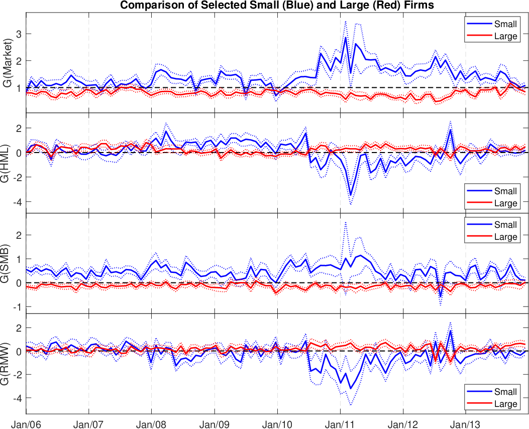
We now focus on two individual stocks’ confidence intervals. We take the two firms that have the highest frequency to be respectively classified in the “large group” and the “small group” by size, and call them “large” and “small”. Figure 3 plots the estimated characteristic betas and the associated confidence intervals of the two firms over time. As for the beta associated with the market factor, while both are positively significant, the characteristic betas of the firm with smaller size are constantly larger than one, making it more sensitive to the changes of market risks than the firm with the larger size. In addition, the pattern shown by the characteristic beta of the SMB factor is similar to Table 1: in the long run, the smaller firm is positively exposed and the larger firm is negatively exposed to the SMB systematic risk.
5.4 Testing characteristic relevance in asset pricing models
We now test the relevance of characteristics on factor betas, an important research question in asset pricing. We consider the linear specification for a common coefficient matrix and test the relevance of each of the characteristics (size, value, momentum and volatility) on the betas. Note that the -th element of , denoted by , represents the effect of characteristic on the the factor beta. Although this specifies a linear function , could include nonlinear (sieve) transformations of each characteristic. Our test is uniformly valid over . To estimate , we use the linear sieve and . Then
We construct the bootstrap confidence intervals for each component of the estimated on each trading day, and calculate the proportion of positive (and negative) significance each year. These results are reported in Table 3. For most of the period, the volatility has a significantly positive effect on the market factor, the value characteristic has a significantly positive effect on the HML factor, and the size characteristic has a significantly negative effect on the SMB factor. These results are consistent with the fitted functions in Figures - (in the appendix). Also note that size has insignificant effects on the market beta. We explain this from two aspects: on one hand, the market beta is mostly affected by the volatility instrument, and once it is conditioned, the size is no longer significant. On the other hand, we focus on firms that constitute to the S&P 500 index, whose sizes are relatively large, and are therefore not essential in explaining the market betas.
| positive significance | negative significance | ||||||||
| characteristics | Mkt | HML | SMB | RMW | Mkt | HML | SMB | RMW | |
| 2008 | |||||||||
| size | 0.024 | 0.036 | 0.000 | 0.048 | 0.000 | 0.215 | 0.984 | 0.128 | |
| value | 0.008 | 0.892 | 0.008 | 0.048 | 0.000 | 0.000 | 0.219 | 0.076 | |
| momentum | 0.004 | 0.044 | 0.159 | 0.315 | 0.139 | 0.450 | 0.187 | 0.060 | |
| volatility | 0.534 | 0.598 | 0.295 | 0.092 | 0.000 | 0.048 | 0.040 | 0.167 | |
| 2011 | |||||||||
| size | 0.000 | 0.052 | 0.000 | 0.088 | 0.000 | 0.139 | 0.976 | 0.052 | |
| value | 0.028 | 0.984 | 0.020 | 0.016 | 0.000 | 0.000 | 0.235 | 0.211 | |
| momentum | 0.000 | 0.032 | 0.175 | 0.191 | 0.008 | 0.371 | 0.072 | 0.064 | |
| volatility | 0.956 | 0.004 | 0.147 | 0.000 | 0.000 | 0.741 | 0.195 | 0.821 | |
| 2012 | |||||||||
| size | 0.000 | 0.048 | 0.000 | 0.155 | 0.000 | 0.171 | 0.920 | 0.044 | |
| value | 0.008 | 0.996 | 0.016 | 0.104 | 0.000 | 0.000 | 0.235 | 0.108 | |
| momentum | 0.080 | 0.024 | 0.100 | 0.004 | 0.000 | 0.355 | 0.175 | 0.522 | |
| volatility | 0.813 | 0.171 | 0.458 | 0.187 | 0.000 | 0.155 | 0.036 | 0.084 | |
Finally, addtional numerical results are presented in the appendix, where we plot the estimated functions fitted by B-splines.
6 Conclusion
This paper studies a conditional factor model with a large number of individuals for high-frequency data. One of the key features of our model is that we specify the factor betas as functions of time-varying observed characteristics that pick up long-run beta movements driven by structural changes in the economic environment and in firm- or industry-specific conditions, plus a remaining (idiosyncratic) component that captures high-frequency movements in beta, which picks up short-run fluctuations in beta in periods of high market volatility. The two components capture different aspects of market beta dynamics. We show that the model can be extended to a more general continuous-time many moment conditions setting, and estimated using two-step GMM setting.
The limiting distribution of the estimated characteristic effect on the betas has a discontinuity when the strength of the idiosyncratic beta is near zero. We provide a uniformly valid inference using a cross-sectional bootstrap procedure for the characteristic betas, and do not need to pretest to know whether or not the idiosyncratic beta exists, or their strengths.
The proposed framework can be extended for inference about general coefficients in other important econometric models, such as discrete time conditional factor models, panel data models with varying coefficients, and nonlinear panel models. In these models, the structural parameter may be decomposed into the sum of a characteristic driven component plus an orthogonal component. An important example would be linear panel data model with varying coefficients. In these models the asymptotic distribution of the estimated characteristic effect would also have a discontinuity, and thus standard “plug-in” inference fails to hold uniformly. The proposed bootstrap framework would then be very useful in these models. We shall leave these studies for future research.
References
- Ait-Sahalia et al. (2014) Ait-Sahalia, Y., Kalnina, I. and Xiu, D. (2014). The idiosyncratic volatility puzzle: A reassessment at high frequency. Tech. rep., Working Paper, University of Chicago.
- Aït-Sahalia and Xiu (2017) Aït-Sahalia, Y. and Xiu, D. (2017). Using principal component analysis to estimate a high dimensional factor model with high-frequency data. Journal of Econometrics 201 384–399.
- Andrews (1999) Andrews, D. W. (1999). Estimation when a parameter is on a boundary. Econometrica 67 1341–1383.
- Andrews (2000) Andrews, D. W. (2000). Inconsistency of the bootstrap when a parameter is on the boundary of the parameter space. Econometrica 68 399–405.
- Andrews (2004) Andrews, D. W. (2004). The block–block bootstrap: improved asymptotic refinements. Econometrica 72 673–700.
- Andrews and Soares (2010) Andrews, D. W. and Soares, G. (2010). Inference for parameters defined by moment inequalities using generalized moment selection. Econometrica 78 119–157.
- Ang et al. (2009) Ang, A., Hodrick, R. J., Xing, Y. and Zhang, X. (2009). High idiosyncratic volatility and low returns: International and further us evidence. Journal of Financial Economics 91 1–23.
- Ang and Kristensen (2012) Ang, A. and Kristensen, D. (2012). Testing conditional factor models. Journal of Financial Economics 106 132–156.
- Avramov and Chordia (2006) Avramov, D. and Chordia, T. (2006). Asset pricing models and financial market anomalies. Review of Financial Studies 19 1001–1040.
- Bai and Liao (2017) Bai, J. and Liao, Y. (2017). Inferences in panel data with interactive effects using large covariance matrices. Journal of Econometrics 200 59–78.
- Bai and Ng (2002) Bai, J. and Ng, S. (2002). Determining the number of factors in approximate factor models. Econometrica 70 191–221.
- Barndorff-Nielsen et al. (2008) Barndorff-Nielsen, O. E., Hansen, P. R., Lunde, A. and Shephard, N. (2008). Designing realized kernels to measure the ex post variation of equity prices in the presence of noise. Econometrica 76 1481–1536.
- Barndorff-Nielsen and Shephard (2004) Barndorff-Nielsen, O. E. and Shephard, N. (2004). Econometric analysis of realized covariation: High frequency based covariance, regression, and correlation in financial economics. Econometrica 72 885–925.
- Bollerslev et al. (2016) Bollerslev, T., Li, S. Z. and Todorov, V. (2016). Roughing up beta: Continuous vs. discontinuous betas, and the cross section of expected stock returns. Journal of Financial Economics 120 464–490.
- Cai et al. (2012) Cai, T. T., Yuan, M. et al. (2012). Adaptive covariance matrix estimation through block thresholding. The Annals of Statistics 40 2014–2042.
- Chamberlain and Rothschild (1983) Chamberlain, G. and Rothschild, M. (1983). Arbitrage, factor structure and mean-variance analyssi in large asset markets. Econometrica 51 1305–1324.
- Chen and Liao (2015) Chen, X. and Liao, Z. (2015). Sieve semiparametric two-step gmm under weak dependence. Journal of Econometrics 189 163–186.
- Chen et al. (2003) Chen, X., Linton, O. and Van Keilegom, I. (2003). Estimation of semiparametric models when the criterion function is not smooth. Econometrica 1591–1608.
- Chen and Pouzo (2012) Chen, X. and Pouzo, D. (2012). Estimation of nonparametric conditional moment models with possibly nonsmooth generalized residuals. Econometrica 80 277–321.
- Chernozhukov et al. (2016) Chernozhukov, V., Chetverikov, D., Demirer, M., Duflo, E., Hansen, C. and Newey, W. K. (2016). Double machine learning for treatment and causal parameters. Tech. rep., cemmap working paper, Centre for Microdata Methods and Practice.
- Cochrane (1996) Cochrane, J. H. (1996). A cross-sectional test of an investment-based asset pricing model. Journal of Political Economy 104 572–621.
- Connor and Korajczyk (1993) Connor, G. and Korajczyk, R. (1993). A test for the number of factors in an approximate factor model. Journal of Finance 48 1263–1291.
- Connor and Korajczyk (1986) Connor, G. and Korajczyk, R. A. (1986). Performance measurement with the arbitrage pricing theory: A new framework for analysis. Journal of financial economics 15 373–394.
- Connor and Linton (2007) Connor, G. and Linton, O. (2007). Semiparametric estimation of a characteristic-based factor model of stock returns. Journal of Empirical Finance 14 694–717.
- Connor et al. (2012) Connor, G., Matthias, H. and Linton, O. (2012). Efficient semiparametric estimation of the fama-french model and extensions. Econometrica 80 713–754.
- Daniel and Titman (1997) Daniel, K. and Titman, S. (1997). Evidence on the characteristics of cross sectional variation in stock returns. the Journal of Finance 52 1–33.
- Darolles et al. (2011) Darolles, S., Fan, Y., Florens, J.-P. and Renault, E. (2011). Nonparametric instrumental regression. Econometrica 79 1541–1565.
- Eilers and Marx (1996) Eilers, P. H. and Marx, B. D. (1996). Flexible smoothing with b-splines and penalties. Statistical science 89–102.
- Fama and French (1992) Fama, E. F. and French, K. R. (1992). The cross-section of expected stock returns. Journal of Finance 47 427–465.
- Fan et al. (2016a) Fan, J., Furger, A. and Xiu, D. (2016a). Incorporating global industrial classification standard into portfolio allocation: A simple factor-based large covariance matrix estimator with high-frequency data. Journal of Business & Economic Statistics 34 489–503.
- Fan et al. (2013) Fan, J., Liao, Y. and Mincheva, M. (2013). Large covariance estimation by thresholding principal orthogonal complements (with discussion). Journal of the Royal Statistical Society, Series B 75 603–680.
- Fan et al. (2016b) Fan, J., Liao, Y. and Wang, W. (2016b). Projected principal component analysis in factor models. Annals of statistics 44 219.
- Fan et al. (2015) Fan, J., Liao, Y. and Yao, J. (2015). Power enhancement in high dimensional cross-sectional tests. Econometrica 83 1497Ð1541.
- Ferson and Harvey (1999) Ferson, W. E. and Harvey, C. R. (1999). Conditioning variables and the cross section of stock returns. The Journal of Finance 54 1325–1360.
- Gagliardini et al. (2016) Gagliardini, P., Ossola, E. and Scaillet, O. (2016). Time-varying risk premium in large cross-sectional equity data sets. Econometrica 84 985–1046.
- Ghysels (1998) Ghysels, E. (1998). On stable factor structures in the pricing of risk: Do time-varying betas help or hurt? The Journal of Finance 53 549–573.
- Hall and Horowitz (2005) Hall, P. and Horowitz, J. L. (2005). Nonparametric methods for inference in the presence of instrumental variables. The Annals of Statistics 33 2904–2929.
- Herskovic et al. (2016) Herskovic, B., Kelly, B., Lustig, H. and Van Nieuwerburgh, S. (2016). The common factor in idiosyncratic volatility: Quantitative asset pricing implications. Journal of Financial Economics 119 249–283.
- Jacod et al. (2009)
Jacod, J., Li, Y., Mykland, P. A.,
Podolskij, M. and Vetter, M. (2009).
Microstructure noise in the continuous case: The pre-averaging
approach.
Stochastic Processes and their Applications 119
2249–2276.
URL http://ideas.repec.org/a/eee/spapps/v119y2009i7p2249-2276.html - Jacod and Protter (2011) Jacod, J. and Protter, P. (2011). Discretization of Processes. Springer.
- Jacod and Rosenbaum (2013) Jacod, J. and Rosenbaum, M. (2013). Quarticity and other functionals of volatility: Efficient estimation. The Annals of Statistics 41 1462–1484.
- Jagannathan and Wang (1996) Jagannathan, R. and Wang, Z. (1996). The conditional capm and the cross-section of expected returns. The Journal of finance 51 3–53.
- Kalnina (2012) Kalnina, I. (2012). Nonparametric tests of time variation in betas. Université de Montréal .
- Kelly et al. (2017) Kelly, B. T., Pruitt, S. and Su, Y. (2017). Instrumented principal component analysis .
- Ketz (2017) Ketz, P. (2017). Testing overidentifying restrictions when the true parameter vector is near or at the boundary of the parameter space. Tech. rep., Working Paper.
- Ketz (2018) Ketz, P. (2018). Subvector inference when the true parameter vector may be near or at the boundary .
- Kim et al. (2018) Kim, S., Korajczyk, R. A. and Neuhierl, A. (2018). Arbitrage portfolios in large panels. Available at SSRN .
- King et al. (1994) King, M., Sentana, E. and Wadhwani, S. (1994). Volatility and links between national stock markets. Econometrica 62 901–33.
- Lahiri (1999) Lahiri, S. N. (1999). Theoretical comparisons of block bootstrap methods. Annals of Statistics 386–404.
- Lettau and Ludvigson (2001) Lettau, M. and Ludvigson, S. (2001). Resurrecting the (c) capm: A cross-sectional test when risk premia are time-varying. Journal of political economy 109 1238–1287.
- Li et al. (2016) Li, J., Todorov, V. and Tauchen, G. (2016). Inference theory for volatility functional dependencies. Journal of Econometrics 193 17–34.
- Li et al. (2017) Li, J., Todorov, V. and Tauchen, G. (2017). Adaptive estimation of continuous-time regression models using high-frequency data. Journal of Econometrics 200 36–47.
- Li et al. (2018) Li, J., Todorov, V. and Tauchen, G. (2018). Jump factor models in large cross-sections.
- Li and Xiu (2016) Li, J. and Xiu, D. (2016). Generalized method of integrated moments for high-frequency data. Econometrica 84 1613–1633.
- Mancini (2001) Mancini, C. (2001). Disentangling the jumps of the diffusion in a geometric jumping Brownian motion. Giornale dell’Istituto Italiano degli Attuari LXIV 19–41.
- Mykland et al. (2006) Mykland, P. A., Zhang, L. et al. (2006). Anova for diffusions and ito processes. The Annals of Statistics 34 1931–1963.
- Newey (1994) Newey, W. K. (1994). The asymptotic variance of semiparametric estimators. Econometrica 1349–1382.
- Newey and Powell (2003) Newey, W. K. and Powell, J. L. (2003). Instrumental variable estimation of nonparametric models. Econometrica 71 1565–1578.
- Pedersen (2017) Pedersen, R. S. (2017). Inference and testing on the boundary in extended constant conditional correlation garch models. Journal of Econometrics 196 23–36.
- Pelger (2016) Pelger, M. (2016). Large-dimensional factor modeling based on high-frequency observations. Working paper.
- Protter (2005) Protter, P. E. (2005). Stochastic Integration and Differential Equations. 2nd ed. Springer.
- Shanken (1990) Shanken, J. (1990). Intertemporal asset pricing: An empirical investigation. Journal of Econometrics 45 99–120.
- Stock and Watson (2002) Stock, J. and Watson, M. (2002). Forecasting using principal components from a large number of predictors. Journal of the American Statistical Association 97 1167–1179.
- White (1980) White, H. (1980). A heteroskedasticity-consistent covariance matrix estimator and a direct test for heteroskedasticity. Econometrica 817–838.
- Zhang et al. (2005) Zhang, L., Mykland, P. A. and Aït-Sahalia, Y. (2005). A tale of two time scales: Determining integrated volatility with noisy high-frequency data. Journal of the American Statistical Association 100 1394–1411.