跳到论文正文
W Papers独立论文阅读器 arXiv:1711.04320 论文正文 计算阅读时间 · 0%
引用这篇论文根据当前论文元数据生成,正式投稿前建议核对。


License: arXiv.org perpetual non-exclusive license
arXiv:1711.04320v2 [math.SG] 18 Jan 2020

Fundamental groups of formal Legendrian and Horizontal embedding spaces

Eduardo Fernández Address: Universidad Complutense de Madrid, Departamento de Álgebra, Geometría y Topología, Facultad de Matemáticas, and Instituto de Ciencias Matemáticas CSIC-UAM-UC3M-UCM, C. Nicolás Cabrera, 13-15, 28049 Madrid, Spain. Email address: eduarf01@ucm.es;eduardo.fernandez@icmat.es , Javier Martínez-Aguinaga Address: Universidad Complutense de Madrid, Departamento de Álgebra, Geometría y Topología, Facultad de Matemáticas, and Instituto de Ciencias Matemáticas CSIC-UAM-UC3M-UCM, C. Nicolás Cabrera, 13-15, 28049 Madrid, Spain. Email address: javier.martinez.aguinaga@icmat.es and Francisco Presas Address: Instituto de Ciencias Matemáticas CSIC-UAM-UC3M-UCM, C. Nicolás Cabrera, 13-15, 28049 Madrid, Spain. Email address: fpresas@icmat.es
Date: August 24, 2026
Abstract.

We compute the fundamental group of each connected component of the space of formal Legendrian embeddings in ℝ3\mathbb{R}^{3}. We use it to show that previous examples in the literature of non trivial loops of Legendrian embeddings are already non trivial at the formal level. Likewise, we compute the fundamental group of the different connected components of the space of formal horizontal embeddings into the standard Engel ℝ4\mathbb{R}^{4}. We check that the natural inclusion of the space of horizontal embeddings into the space of formal horizontal embeddings induces an isomorphism at π1\pi_{1}–level.

2010 Mathematics Subject Classification
Primary: 58A30, 57R17.

1. Introduction.

The computation of the homotopy type of the space of Legendrian embeddings into a contact 33–fold has a long story. For a while, it was thought that the computation could be made at the formal level. We mean by that that the inclusion of the space of Legendrian embeddings into the space of formal Legendrian embeddings, ie the space of pairs: smooth embedding and formal Legendrian derivative, was a weak homotopy equivalence. This was proven to be wrong in the key article of D. Bennequin [4]; in which it was shown that the formal space associated to the standard contact ℝ3{\mathbb{R}}^{3} possesses some connected components that are not representable by Legendrian knots. In other words, the restriction of the induced map of the inclusion at π0\pi_{0}–level was not surjective. This was the first hint of ridigity phenomena in contact topology. Later on, there has been an industry checking how far the inclusion map is at π0\pi_{0}–level from being injective or surjective, see, eg, the work of Chekanov [7], Ding and Geiges [8], Eliashberg and Fraser [10], Etnyre and Honda [13] or Osváth, Szabó and Thurston [29].

The next step was the study of higher homotopy groups. This was developed by Kálmán [23] in dimension 33 using pseudoholomorphic curves invariants and by Sabloff and Sullivan [28] in dimension 2​n+12n+1, n>1n>1, using generating function invariants. However, they just checked that several non trivial loops in the space of Legendrian embeddings were trivial as elements in the fundamental group of the space of smooth embeddings. We show that all Kálmán’s examples are non trivial in the space of formal Legendrian embeddings, see Section 4. This makes unnecessary the use of sophisticated invariants to compute these examples. In order to do that, we compute the fundamental group of the space of formal Legendrian embeddings. This is the content of Section 3.

Moreover, the analogous problem for horizontal embeddings into Engel manifolds satisfies an hh–principle at π0\pi_{0}–level, eg see Adachi [1], Geiges [16] or del Pino and Presas [27]. In Section 5, we compute the fundamental group of the space of formal horizontal embeddings into the standard Engel ℝ4{\mathbb{R}}^{4}. We check that it is ℤ⊕ℤ2{\mathbb{Z}}\oplus{\mathbb{Z}}_{2} where the first component is a rotation invariant that captures the formal immersion class of the loop and the second component captures the formal embedding class of the loop. In Section 6, we provide a way of combinatorially computing this ℤ2{\mathbb{Z}}_{2}–invariant.

Finally, in Section 7, we check that the formal fundamental group is isomorphic to the fundamental group, ie the ℤ2{\mathbb{Z}}_{2}–invariant and the rotation invariant completely classify the elements of the fundamental group of horizontal embeddings. Independently, Casals and del Pino have shown that there is a full hh–principle for horizontal embeddings [6]. Although our proof is more specific, it has the advantage of not using the topology of the space of smooth embeddings. Therefore, we reprove as a corollary that the space of smooth embeddings of circles into ℝ4{\mathbb{R}}^{4} is simply connected, see Budney [5].

The methods developed in this article may allow to compute higher rank homotopy groups of the space of embeddings of the circle in ℝ4{\mathbb{R}}^{4}. The strategy that we are pursuing in a forthcoming project is based on the following facts. First, we compute the higher homotopy groups of the space of horizontal embeddings by the geometrical method developed in this article, that is heavily simplified thanks to the work of Igusa [22]. Secondly, we use [6] in order to state that the previous computations are also computing homotopy groups of the formal horizontal embedding space. Finally, by using obstruction theory, see Hatcher [19, Chapter 4.3], we isolate the homotopy groups of the space of smooth embeddings.

Acknowledgements: The authors are extremely grateful to R. Casals, V. Ginzburg and A. Del Pino for several discussions clarifying the paper. Also, they thank A. Hatcher for pointing out the useful reference [5]. Daniel Álvarez-Gavela has helped as quite a lot with enjoyable meetings whenever he comes to Madrid, he has pointed out several sharp remarks. The third author is also grateful to the organizers of the Engel Structures workshop held in April 2017 (American Institute of Mathematics, San Jose, California) for providing a nice environment in which this article was discussed. Last, but not least, we want to thank the excellent job that the referees have done: they have produced three long and deep reports that have helped to improve the readability of the paper a lot, not to speak of its soundness.

The authors are supported by the Spanish Research Projects SEV–2015–0554, MTM2016–79400–P, and MTM2015–72876–EXP. The first author is supported by a Master–Severo Ochoa grant and by Beca de Personal Investigador en Formación UCM. The second author is funded by Programa Predoctoral de Formación de Personal Investigador No Doctor del Departamento de Educación del Gobierno Vasco.

2. Spaces of embeddings of the circle into euclidean space.

Denote by 𝔈​𝔪​𝔟​(N,M){\mathfrak{Emb}}(N,M) the space of embeddings of a manifold NN into a manifold MM equipped with the CrC^{r}–topology, r≥5r\geq 5.

2.1. The space 𝔈​𝔪​𝔟​(𝕊1,ℝ3){\mathfrak{Emb}}({\mathbb{S}}^{1},{\mathbb{R}}^{3}).

Theorem 2.1.1 (Hatcher, [18] Apendix: equivalence (15)(15)).

The space of parametrized unknotted circles in ℝ3{\mathbb{R}}^{3} has the homotopy type of SO⁡(3)\operatorname{SO}(3).

The group SO⁡(4)\operatorname{SO}(4) acts freely on the connected component 𝔈​𝔪​𝔟p,q​(𝕊1,𝕊3)⊆𝔈​𝔪​𝔟​(𝕊1,𝕊3){\mathfrak{Emb}}_{p,q}({\mathbb{S}}^{1},{\mathbb{S}}^{3})\subseteq{\mathfrak{Emb}}({\mathbb{S}}^{1},{\mathbb{S}}^{3}) of the parametrized (p,q)(p,q) torus knots as

SO⁡(4)×𝔈​𝔪​𝔟p,q​(𝕊1,𝕊3)⟶𝔈​𝔪​𝔟p,q​(𝕊1,𝕊3)(A,γ)⟼A⋅γ.\begin{array}[]{rccl}\operatorname{SO}(4)\times{\mathfrak{Emb}}_{p,q}({\mathbb{S}}^{1},{\mathbb{S}}^{3})&\longrightarrow&{\mathfrak{Emb}}_{p,q}({\mathbb{S}}^{1},{\mathbb{S}}^{3})\\ (A,\gamma)&\longmapsto&A\cdot\gamma.\end{array}

Thus, we have an inclusion SO⁡(4)↪𝔈​𝔪​𝔟p,q​(𝕊1,𝕊3)\operatorname{SO}(4)\hookrightarrow{\mathfrak{Emb}}_{p,q}({\mathbb{S}}^{1},{\mathbb{S}}^{3}). The following result holds:

Theorem 2.1.2 (Hatcher, [20] Theorem 11).

The inclusion SO⁡(4)↪𝔈​𝔪​𝔟p,q​(𝕊1,𝕊3)\operatorname{SO}(4)\hookrightarrow{\mathfrak{Emb}}_{p,q}({\mathbb{S}}^{1},{\mathbb{S}}^{3}) is a homotopy equivalence.

As a consequence of these results we obtain that

Corollary 2.1.3.

Let 𝔈​𝔪​𝔟0​(𝕊1,ℝ3),𝔈​𝔪​𝔟p,q​(𝕊1,ℝ3)⊆𝔈​𝔪​𝔟​(𝕊1,ℝ3){\mathfrak{Emb}}_{0}({\mathbb{S}}^{1},{\mathbb{R}}^{3}),{\mathfrak{Emb}}_{p,q}({\mathbb{S}}^{1},{\mathbb{R}}^{3})\subseteq{\mathfrak{Emb}}({\mathbb{S}}^{1},{\mathbb{R}}^{3}) be the connected component of the parametrized unknots or of the parametrized (p,q)(p,q) torus knots, respectively. The fundamental groups of these spaces are given by

  • •

    π1​(𝔈​𝔪​𝔟0​(𝕊1,ℝ3))≅ℤ2\pi_{1}({\mathfrak{Emb}}_{0}({\mathbb{S}}^{1},{\mathbb{R}}^{3}))\cong{\mathbb{Z}}_{2},

  • •

    π1​(𝔈​𝔪​𝔟p,q​(𝕊1,ℝ3))≅Gp,q⋊ℤ2\pi_{1}({\mathfrak{Emb}}_{p,q}({\mathbb{S}}^{1},{\mathbb{R}}^{3}))\cong G_{p,q}\rtimes{\mathbb{Z}}_{2},

where Gp,qG_{p,q} is the knot group of the (p,q)(p,q) torus knot.

Proof.

The case of the connected component 𝔈​𝔪​𝔟0​(𝕊1,ℝ3){\mathfrak{Emb}}_{0}({\mathbb{S}}^{1},{\mathbb{R}}^{3}) follows from Theorem 2.1.1.

We need to study the connected component 𝔈​𝔪​𝔟p,q​(𝕊1,ℝ3){\mathfrak{Emb}}_{p,q}({\mathbb{S}}^{1},{\mathbb{R}}^{3}) to conclude the proof. Consider the following space

𝒮⁡t​e​r​e​op,q={(γ,x):x∉Image⁡(γ)}⊆𝔈​𝔪​𝔟p,q​(𝕊1,𝕊3)×𝕊3.\operatorname{\mathcal{S}}tereo_{p,q}=\{(\gamma,x):x\notin{\operatorname{Image}}(\gamma)\}\subseteq{\mathfrak{Emb}}_{p,q}({\mathbb{S}}^{1},{\mathbb{S}}^{3})\times{\mathbb{S}}^{3}.

We have two natural fibrations associated to the projection maps

𝔈​𝔪​𝔟p,q​(𝕊1,ℝ3)\textstyle{{\mathfrak{Emb}}_{p,q}({\mathbb{S}}^{1},{\mathbb{R}}^{3})\ignorespaces\ignorespaces\ignorespaces\ignorespaces}𝒮⁡t​e​r​e​op,q\textstyle{\operatorname{\mathcal{S}}tereo_{p,q}\ignorespaces\ignorespaces\ignorespaces\ignorespaces}𝕊3\Kp,q\textstyle{{\mathbb{S}}^{3}\backslash K_{p,q}\ignorespaces\ignorespaces\ignorespaces\ignorespaces}𝒮⁡t​e​r​e​op,q\textstyle{\operatorname{\mathcal{S}}tereo_{p,q}\ignorespaces\ignorespaces\ignorespaces\ignorespaces}𝕊3\textstyle{{\mathbb{S}}^{3}}𝔈​𝔪​𝔟p,q​(𝕊1,𝕊3)\textstyle{{\mathfrak{Emb}}_{p,q}({\mathbb{S}}^{1},{\mathbb{S}}^{3})}

where Kp,qK_{p,q} is the image of the standard (p,q)(p,q) torus knot in 𝕊3{\mathbb{S}}^{3}. From the first fibration we obtain

π1​(𝔈​𝔪​𝔟p,q​(𝕊1,ℝ3))≅π1​(𝒮⁡t​e​r​e​op,q).\pi_{1}({\mathfrak{Emb}}_{p,q}({\mathbb{S}}^{1},{\mathbb{R}}^{3}))\cong\pi_{1}(\operatorname{\mathcal{S}}tereo_{p,q}).

Moreover, from the second one and the fact that 𝔈​𝔪​𝔟p,q​(𝕊1,𝕊3){\mathfrak{Emb}}_{p,q}({\mathbb{S}}^{1},{\mathbb{S}}^{3}) has the homotopy type of SO⁡(4)\operatorname{SO}(4) (Theorem 2.1.2), we obtain that the sequence

0\textstyle{0\ignorespaces\ignorespaces\ignorespaces\ignorespaces}Gp,q\textstyle{G_{p,q}\ignorespaces\ignorespaces\ignorespaces\ignorespaces}π1​(𝒮⁡t​e​r​e​op,q)\textstyle{\pi_{1}(\operatorname{\mathcal{S}}tereo_{p,q})\ignorespaces\ignorespaces\ignorespaces\ignorespaces}ℤ2\textstyle{{\mathbb{Z}}_{2}\ignorespaces\ignorespaces\ignorespaces\ignorespaces}0\textstyle{0}

is exact. Now, it is a simple exercise to check that this sequence is right split. ∎

2.2. The space 𝔈​𝔪​𝔟​(𝕊1,ℝ4){\mathfrak{Emb}}({\mathbb{S}}^{1},{\mathbb{R}}^{4}).

A long embedding of ℝ{\mathbb{R}} into ℝ4{\mathbb{R}}^{4} is an embedding γ:ℝ→ℝ4\gamma:{\mathbb{R}}\rightarrow{\mathbb{R}}^{4} that coincides with the standard inclusion ℝ↪ℝ×ℝ3=ℝ4{\mathbb{R}}\hookrightarrow{\mathbb{R}}\times{\mathbb{R}}^{3}={\mathbb{R}}^{4} outside a compact neighborhood of the origin. Let 𝔏​𝔈​𝔪​𝔟​(ℝ,ℝ4){\mathfrak{LEmb}}({\mathbb{R}},{\mathbb{R}}^{4}) denote the space of long embeddings of ℝ{\mathbb{R}} into ℝ4{\mathbb{R}}^{4}.

Lemma 2.2.1 (Budney).

𝔈​𝔪​𝔟​(𝕊1,ℝ4){\mathfrak{Emb}}({\mathbb{S}}^{1},{\mathbb{R}}^{4}) is homotopy equivalent to 𝕊3×𝕊2×𝔏​𝔈​𝔪​𝔟​(ℝ,ℝ4){\mathbb{S}}^{3}\times{\mathbb{S}}^{2}\times{\mathfrak{LEmb}}({\mathbb{R}},{\mathbb{R}}^{4}).

Proof.

It follows from [5, Proposition 2.2] that 𝔈​𝔪​𝔟​(𝕊1,ℝ4){\mathfrak{Emb}}({\mathbb{S}}^{1},{\mathbb{R}}^{4}) is homotopy equivalent to (SO⁡(4)×𝒮⁡t​e​r​e​o~)/SO⁡(3)(\operatorname{SO}(4)\times\widetilde{\operatorname{\mathcal{S}}tereo})/\operatorname{SO}(3), where 𝒮⁡t​e​r​e​o~={(p,f):p∉Image⁡(f)}⊆ℝ4×𝔏​𝔈​𝔪​𝔟​(ℝ,ℝ4)\widetilde{\operatorname{\mathcal{S}}tereo}=\{(p,f):p\notin{\operatorname{Image}}(f)\}\subseteq{\mathbb{R}}^{4}\times{\mathfrak{LEmb}}({\mathbb{R}},{\mathbb{R}}^{4}). Observe that the quaternion structure in ℝ4​(i,j,k){\mathbb{R}}^{4}(i,j,k) induces a homotopy equivalence 𝕊3×𝒮⁡t​e​r​e​o~→(SO⁡(4)×𝒮⁡t​e​r​e​o~)/SO⁡(3);(v,(p,f))↦[((v|i​v​|j​v|​k​v),(p,f))]{\mathbb{S}}^{3}\times\widetilde{\operatorname{\mathcal{S}}tereo}\rightarrow(\operatorname{SO}(4)\times\widetilde{\operatorname{\mathcal{S}}tereo})/\operatorname{SO}(3);(v,(p,f))\mapsto[((v|iv|jv|kv),(p,f))]. Finally, the natural fibration 𝒮⁡t​e​r​e​o~↦𝔏​𝔈​𝔪​𝔟​(ℝ,ℝ4)\widetilde{\operatorname{\mathcal{S}}tereo}\mapsto{\mathfrak{LEmb}}({\mathbb{R}},{\mathbb{R}}^{4}) has fiber homotopy equivalent to 𝕊2{\mathbb{S}}^{2}, since the space 𝔏​𝔈​𝔪​𝔟​(ℝ,ℝ4){\mathfrak{LEmb}}({\mathbb{R}},{\mathbb{R}}^{4}) is connected and ℝ4\ℝ∼h.e.𝕊2{\mathbb{R}}^{4}\backslash{\mathbb{R}}\stackrel{{\scriptstyle h.e.}}{{\sim}}{\mathbb{S}}^{2}. Moreover the fibration homotopically splits since given any family φ:𝕊k→𝔏​𝔈​𝔪​𝔟​(ℝ,ℝ4)\varphi:{\mathbb{S}}^{k}\rightarrow{\mathfrak{LEmb}}({\mathbb{R}},{\mathbb{R}}^{4}), it admits a lift given by φε:𝕊k→𝒮⁡t​e​r​e​o~;z↦(φ⁡(z)​(0)+ε⋅i​φ​(z)′​(0),φ⁡(z))\varphi_{\varepsilon}:{\mathbb{S}}^{k}\rightarrow\widetilde{\operatorname{\mathcal{S}}tereo};z\mapsto(\varphi(z)(0)+\varepsilon\cdot i\varphi(z)^{\prime}(0),\varphi(z)) for some ε>0\varepsilon>0 small enough. ∎

Let us geometrically explain the homotopy equivalence stated in the last Lemma. Let {e1,e2,e3,e4}\{e_{1},e_{2},e_{3},e_{4}\} be the canonical basis of ℝ4{\mathbb{R}}^{4} and write ℝ4=ℝ⁡⟨e1⟩×ℝ3​⟨e2,e3,e4⟩{\mathbb{R}}^{4}={\mathbb{R}}\langle e_{1}\rangle\times{\mathbb{R}}^{3}\langle e_{2},e_{3},e_{4}\rangle. From a long embedding we obtain an embedding of 𝕊1{\mathbb{S}}^{1} into ℝ4{\mathbb{R}}^{4} closing it in the plane ⟨e1,p⟩\langle e_{1},p\rangle, where p∈𝕊2⊆ℝ3​⟨e2,e3,e4⟩p\in{\mathbb{S}}^{2}\subseteq{\mathbb{R}}^{3}\langle e_{2},e_{3},e_{4}\rangle. Finally, the 𝕊3{\mathbb{S}}^{3} factor acts by quaternionic multiplication on a fixed embedding.

It follows that π2​(𝔈​𝔪​𝔟​(𝕊1,ℝ4))≅π2​(𝕊2)⊕π2​(𝔏​𝔈​𝔪​𝔟​(ℝ,ℝ4))≅ℤ⊕π2​(𝔏​𝔈​𝔪​𝔟​(ℝ,ℝ4))\pi_{2}({\mathfrak{Emb}}({\mathbb{S}}^{1},{\mathbb{R}}^{4}))\cong\pi_{2}({\mathbb{S}}^{2})\oplus\pi_{2}({\mathfrak{LEmb}}({\mathbb{R}},{\mathbb{R}}^{4}))\cong{\mathbb{Z}}\oplus\pi_{2}({\mathfrak{LEmb}}({\mathbb{R}},{\mathbb{R}}^{4})). We provide an explicit construction of the generator of the ℤ{\mathbb{Z}} factor in this decomposition. For every point p∈𝕊2⊆ℝ3​⟨e2,e3,e4⟩p\in{\mathbb{S}}^{2}\subseteq{\mathbb{R}}^{3}\langle e_{2},e_{3},e_{4}\rangle take the standard parametrized unknot in span⁡{e1,p}\operatorname{span}\{e_{1},p\} centered at pp and tangent to the line generated by e1e_{1} at 00. This gives us a 22–parametric family of knots, that we denote by SUS_{U}, whose homotopy class is the generator (1,0)(1,0) of π2​(𝔈​𝔪​𝔟​(𝕊1,ℝ4))\pi_{2}({\mathfrak{Emb}}({\mathbb{S}}^{1},{\mathbb{R}}^{4})). Explicitly, SUS_{U} is defined as:

SU:𝕊2⟶𝔈​𝔪​𝔟​(𝕊1,ℝ4)p⟼γp​(t)\begin{array}[]{rccl}S_{U}\colon&{\mathbb{S}}^{2}&\longrightarrow&{\mathfrak{Emb}}({\mathbb{S}}^{1},{\mathbb{R}}^{4})\\ &p&\longmapsto&\gamma_{p}(t)\end{array}

where, if p=(λ1,λ2,λ3)∈𝕊2p=(\lambda_{1},\lambda_{2},\lambda_{3})\in{\mathbb{S}}^{2},

γp​(t)=sin⁡(2​π​t)​e1+(1−cos⁡(2​π​t))​(λ1​e2+λ2​e3+λ3​e4).\gamma_{p}(t)=\sin(2\pi t)e_{1}+(1-\cos(2\pi t))(\lambda_{1}e_{2}+\lambda_{2}e_{3}+\lambda_{3}e_{4}).
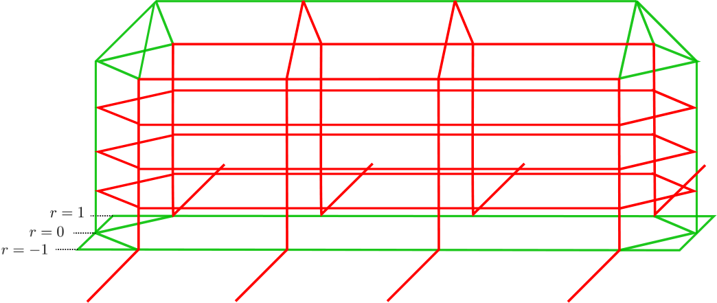
Refer to caption
Figure 1. Construction of SUS_{U} (schematically).
Remark 2.2.2.

In [5, Proposition 3.9(4)] Budney shows that the space 𝔈​𝔪​𝔟​(𝕊1,ℝ4){\mathfrak{Emb}}({\mathbb{S}}^{1},{\mathbb{R}}^{4}) is simply connected and π2​(𝔈​𝔪​𝔟​(𝕊1,ℝ4))≅ℤ⊕ℤ\pi_{2}({\mathfrak{Emb}}({\mathbb{S}}^{1},{\mathbb{R}}^{4}))\cong{\mathbb{Z}}\oplus{\mathbb{Z}}. Moreover, he provides an explicit construction of the second generator of the second homotopy group ([5, Theorem 3.13]).

In section 7 we provide an alternative proof of the fact that 𝔈​𝔪​𝔟​(𝕊1,ℝ4){\mathfrak{Emb}}({\mathbb{S}}^{1},{\mathbb{R}}^{4}) is simply connected based on the techniques developed in this paper.

3. Formal Legendrian Embeddings in ℝ3{\mathbb{R}}^{3}.

We denote by ξ\xi the standard contact structure in ℝ3​(x,y,z){\mathbb{R}}^{3}(x,y,z) given by ξ=ker⁡(d​z−y​d​x)\xi=\ker(dz-ydx). Throughout the Section we fix the Legendrian framing ∂y\partial_{y}.11 1 Observe that ξ\xi is naturally (co)oriented by the contact form d​z−y​d​xdz-ydx and, thus, ∂y\partial_{y} determines a unique oriented framing up to homotopy.

3.1. Formal Legendrian Embeddings in ℝ3{\mathbb{R}}^{3}.

Definition 3.1.1.

An immersion γ:𝕊1→ℝ3\gamma:{\mathbb{S}}^{1}\rightarrow{\mathbb{R}}^{3} is said to be Legendrian if γ′​(t)∈ξγ⁡(t)\gamma^{\prime}(t)\in\xi_{\gamma(t)} for all t∈𝕊1t\in{\mathbb{S}}^{1}. If γ\gamma is an embedding, we say it is a Legendrian embedding.

Definition 3.1.2.

A formal Legendrian immersion in ℝ3{\mathbb{R}}^{3} is a pair (γ,F)(\gamma,F) such that:

  • (i)

    γ:𝕊1→ℝ3\gamma:{\mathbb{S}}^{1}\rightarrow{\mathbb{R}}^{3} is a smooth map.

  • (ii)

    F:𝕊1→γ∗​(T​ℝ3\{0})F:{\mathbb{S}}^{1}\rightarrow\gamma^{*}(T{\mathbb{R}}^{3}\backslash\{0\}) satisfies F⁡(t)∈ξγ⁡(t)F(t)\in\xi_{\gamma(t)}.

A formal Legendrian embedding in ℝ3{\mathbb{R}}^{3} is a pair (γ,Fs)(\gamma,F_{s}), satisfying:

  • (i)

    γ:𝕊1→ℝ3\gamma:{\mathbb{S}}^{1}\rightarrow{\mathbb{R}}^{3} is an embedding.

  • (ii)

    Fs:𝕊1→γ∗​(T​ℝ3∖{0})F_{s}:{\mathbb{S}}^{1}\rightarrow\gamma^{*}(T{\mathbb{R}}^{3}\setminus\{0\}), is a 11–parametric family, s∈[0,1]s\in[0,1], such that F0=γ′F_{0}=\gamma^{\prime} and F1​(t)∈ξγ⁡(t)F_{1}(t)\in\xi_{\gamma(t)}.

Use the framing ⟨∂y⟩\langle\partial_{y}\rangle to trivialize the contact distribution understood as a bundle. This provides a bundle isomorphism ξ≃ℝ2\xi\simeq{\mathbb{R}}^{2}. From now on, we will understand the map F:𝕊1→𝕊1≡𝕊2∩ℝ2F:{\mathbb{S}}^{1}\rightarrow{\mathbb{S}}^{1}\equiv{\mathbb{S}}^{2}\cap{\mathbb{R}}^{2} and the family Fs:𝕊1→𝕊2F_{s}:{\mathbb{S}}^{1}\rightarrow{\mathbb{S}}^{2} with F1:𝕊1→𝕊1≡𝕊2∩ℝ2F_{1}:{\mathbb{S}}^{1}\rightarrow{\mathbb{S}}^{1}\equiv{\mathbb{S}}^{2}\cap{\mathbb{R}}^{2}. We say that an immersion is strict if it is a non injective map.

Denote by 𝔏​𝔢​𝔤​ℑ​𝔪​𝔪​(ℝ3){\mathfrak{LegImm}}({\mathbb{R}}^{3}) the space of Legendrian immersions in ℝ3{\mathbb{R}}^{3}, by 𝔏​𝔢​𝔤​(ℝ3){\mathfrak{Leg}}({\mathbb{R}}^{3}) the space of Legendrian embeddings in ℝ3{\mathbb{R}}^{3} and by 𝔏​𝔢​𝔤​ℑ​𝔪​𝔪strict​(ℝ3)=𝔏​𝔢​𝔤​ℑ​𝔪​𝔪​(ℝ3)\𝔏​𝔢​𝔤​(ℝ3){\mathfrak{LegImm}^{\textbf{strict}}}({\mathbb{R}}^{3})={\mathfrak{LegImm}}({\mathbb{R}}^{3})\backslash{\mathfrak{Leg}}({\mathbb{R}}^{3}) the space of strict Legendrian immersions. Denote also by 𝔉​𝔏​𝔢​𝔤​ℑ​𝔪​𝔪​(ℝ3){\mathfrak{FLegImm}}({\mathbb{R}}^{3}) the space of formal Legendrian immersions and by 𝔉​𝔏​𝔢​𝔤​(ℝ3){\mathfrak{FLeg}}({\mathbb{R}}^{3}) the space of formal Legendrian embeddings. These definitions make sense for immersions and embeddings of the interval. We define 𝔏​𝔢​𝔤​ℑ​𝔪​𝔪​([0,1],ℝ3){\mathfrak{LegImm}}([0,1],{\mathbb{R}}^{3}), 𝔏​𝔢​𝔤​([0,1],ℝ3){\mathfrak{Leg}}([0,1],{\mathbb{R}}^{3}), 𝔏​𝔢​𝔤​ℑ​𝔪​𝔪strict​([0,1],ℝ3){\mathfrak{LegImm}^{\textbf{strict}}}([0,1],{\mathbb{R}}^{3}), 𝔉​𝔏​𝔢​𝔤​ℑ​𝔪​𝔪​([0,1],ℝ3){\mathfrak{FLegImm}}([0,1],{\mathbb{R}}^{3}) and 𝔉​𝔏​𝔢​𝔤​([0,1],ℝ3){\mathfrak{FLeg}}([0,1],{\mathbb{R}}^{3}) analogously.

Remark 3.1.3.

The space of CrC^{r}–maps ℳ⁡𝔞​𝔭​𝔰r​(𝕊1,ℝ3)\operatorname{\mathcal{M}}\mathfrak{aps}^{r}({\mathbb{S}}^{1},{\mathbb{R}}^{3}) endowed with the CrC^{r}–topology is a Banach vector space. It has an open submanifold that is the space of immersions ℑ​𝔪​𝔪r​(𝕊1,ℝ3){\mathfrak{Imm}}^{r}({\mathbb{S}}^{1},{\mathbb{R}}^{3}). Denote by α\alpha the standard contact form in ℝ3{\mathbb{R}}^{3}; ie ker⁡(α)=ξ\ker(\alpha)=\xi. There is a smooth submersion α~:ℳ⁡𝔞​𝔭​𝔰r​(𝕊1,ℝ3)→Ω1​(𝕊1),γ↦γ∗​(α)\tilde{\alpha}:\operatorname{\mathcal{M}}\mathfrak{aps}^{r}({\mathbb{S}}^{1},{\mathbb{R}}^{3})\to\Omega^{1}({\mathbb{S}}^{1}),\gamma\mapsto\gamma^{*}(\alpha). We have that 𝔏​𝔢​𝔤​ℑ​𝔪​𝔪r​(ℝ3){\mathfrak{LegImm}}^{r}({\mathbb{R}}^{3}) is a Banach submanifold of ℑ​𝔪​𝔪r​(𝕊1,ℝ3){\mathfrak{Imm}}^{r}({\mathbb{S}}^{1},{\mathbb{R}}^{3}) (see Lang [24, Corollary 5.7, page 19]). Whenever we speak about families of curves in the space of Legendrians we are implicitly asumming this Banach structure. This means that our maps are CrC^{r} instead of smooth but all the definitions in the paper make sense for CrC^{r}–maps whenever r≥5r\geq 5. To simplify the notation we will be writing smooth maps instead of C5C^{5}–maps unless it is stated otherwise. The bound r≥5r\geq 5 comes from the fact that we are considering 33–dimensional families of Legendrians. In order to locally classify them we need to consider up to 44 derivatives of their front projection (55 of the original Legendrians).

It is important to note that any γ∈𝔏​𝔢​𝔤​ℑ​𝔪​𝔪r​(ℝ3)\gamma\in{\mathfrak{LegImm}}^{r}({\mathbb{R}}^{3}) admits a particular type of immersed chart φγ\varphi_{\gamma}, called a Weinstein chart, which identifies via a immersed contactomorphism a tubular neighborhood of the zero section of the jet space J1​(𝕊1)J^{1}({\mathbb{S}}^{1}) (see Geiges [15, Example 2.5.11]) with a tubular neighborhood of γ⁡(𝕊1)\gamma({\mathbb{S}}^{1}). This construction provides the local structure produced by the Implicit Function Theorem applied in the last paragraph. We can just check that the exponential map in a CrC^{r}–neighborhood of γ\gamma is defined as the following construction: take f∈ℳ⁡𝔞​𝔭​𝔰r​(𝕊1,ℝ)f\in\operatorname{\mathcal{M}}\mathfrak{aps}^{r}({\mathbb{S}}^{1},{\mathbb{R}}), a map f~∈ℳ⁡𝔞​𝔭​𝔰r​(𝕊1,𝕊1)\tilde{f}\in\operatorname{\mathcal{M}}\mathfrak{aps}^{r}({\mathbb{S}}^{1},{\mathbb{S}}^{1}) such that f~​(θ)=θ+f​(θ)\tilde{f}(\theta)=\theta+f(\theta). Then, the map is defined as

(1) 𝒞:𝒰⊆ℳ⁡𝔞​𝔭​𝔰r​(𝕊1,ℝ)×ℳ⁡𝔞​𝔭​𝔰r​(𝕊1,ℝ)⟶𝒱⊆𝔏​𝔢​𝔤​ℑ​𝔪​𝔪r​(ℝ3)(f,g)⟼φγ−1∘j1​(g∘f~).\begin{array}[]{rccl}\mathcal{C}\colon&\mathcal{U}\subseteq\operatorname{\mathcal{M}}\mathfrak{aps}^{r}({\mathbb{S}}^{1},{\mathbb{R}})\times\operatorname{\mathcal{M}}\mathfrak{aps}^{r}({\mathbb{S}}^{1},{\mathbb{R}})&\longrightarrow&\mathcal{V}\subseteq{\mathfrak{LegImm}}^{r}({\mathbb{R}}^{3})\\ &(f,g)&\longmapsto&\varphi_{\gamma}^{-1}\circ j^{1}(g\circ\tilde{f}).\end{array}

Note that this is a local chart (ie a diffeomorphism). However, if we consider r=∞r=\infty the previous map is not surjective in the reparametrizations direction since it is well-known that the action of the Lie algebra of Diff⁡(𝕊1)\operatorname{Diff}({\mathbb{S}}^{1}) is not surjective on Diff⁡(𝕊1)\operatorname{Diff}({\mathbb{S}}^{1}). On the other hand, if we quotient out 𝔏​𝔢​𝔤​ℑ​𝔪​𝔪∞​(ℝ3){\mathfrak{LegImm}}^{\infty}({\mathbb{R}}^{3}) by the action of Diff⁡(𝕊1)\operatorname{Diff}({\mathbb{S}}^{1}), ie we consider non–parametrized Legendrians, the map is a local diffeomorphism. This is an obvious consequence of the characterization of the Legendrian curves in J1​(𝕊1)J^{1}({\mathbb{S}}^{1}) as graphs of smooth functions. We use r<∞r<\infty in order to make sure that the parametrizations are surjective. We do not forget about reparametrizations because they are important in our algebraic topology arguments.

From now on we will skip the index r=5r=5 in all the statements, unless it is not clear from the context.

All the spaces of Legendrians are equipped with the CrC^{r}–topology. On the other hand, the spaces of formal Legendrians are equipped with the product topology that is the CrC^{r}–topology for the first factor (the smooth immersion/embedding) and the Cr−1C^{r-1}–topology for the second factor (the formal derivative).

Remark 3.1.4.

It is well–known that hh–principle holds for Legendrian immersions (see, eg, Eliashberg and Mishachev [11]). Hence, π0​(𝔏​𝔢​𝔤​ℑ​𝔪​𝔪​(ℝ3))≅ℤ\pi_{0}({\mathfrak{LegImm}}({\mathbb{R}}^{3}))\cong{\mathbb{Z}}, π1​(𝔏​𝔢​𝔤​ℑ​𝔪​𝔪​(ℝ3))≅ℤ\pi_{1}({\mathfrak{LegImm}}({\mathbb{R}}^{3}))\cong{\mathbb{Z}} and πk​(𝔏​𝔢​𝔤​ℑ​𝔪​𝔪​(ℝ3))=0,\pi_{k}({\mathfrak{LegImm}}({\mathbb{R}}^{3}))=0, for all k≥2k\geq 2. The connected components of 𝔏​𝔢​𝔤​ℑ​𝔪​𝔪​(ℝ3){\mathfrak{LegImm}}({\mathbb{R}}^{3}) are given by the rotation number. The rotation number of an Legendrian immersion γ\gamma is Rot(γ)=deg(γ′:𝕊1→𝕊1)\operatorname{Rot}(\gamma)=\deg(\gamma^{\prime}:{\mathbb{S}}^{1}\rightarrow{\mathbb{S}}^{1}). Let us explain the group π1​(𝔏​𝔢​𝔤​ℑ​𝔪​𝔪​(ℝ3))≅ℤ\pi_{1}({\mathfrak{LegImm}}({\mathbb{R}}^{3}))\cong{\mathbb{Z}}. Take a loop γθ\gamma^{\theta} in 𝔏​𝔢​𝔤​ℑ​𝔪​𝔪​(ℝ3){\mathfrak{LegImm}}({\mathbb{R}}^{3}), the integer is just RotL⁡(γθ)=deg⁡(θ↦(γθ)′​(0))\operatorname{Rot}_{L}(\gamma^{\theta})=\deg(\theta\mapsto(\gamma^{\theta})^{\prime}(0)), we call this number rotation number of the loop. These invariants make sense in the formal case and the definitions are the obvious ones.

3.2. The space 𝔉​𝔏​𝔢​𝔤​(ℝ3){\mathfrak{FLeg}}({\mathbb{R}}^{3}).

Consider the space 𝔉​𝔏​𝔢​𝔤^(ℝ3)={(γ,F)|γ∈𝔈𝔪𝔟(𝕊1,ℝ3),F∈ℳ𝔞𝔭𝔰(𝕊1,𝕊1)}{\widehat{\mathfrak{FLeg}}}({\mathbb{R}}^{3})=\{(\gamma,F)|\gamma\in{\mathfrak{Emb}}({\mathbb{S}}^{1},{\mathbb{R}}^{3}),F\in\operatorname{\mathcal{M}}\mathfrak{aps}({\mathbb{S}}^{1},{\mathbb{S}}^{1})\}. We have a natural fibration 𝔉​𝔏​𝔢​𝔤​(ℝ3)→𝔉​𝔏​𝔢​𝔤^​(ℝ3){\mathfrak{FLeg}}({\mathbb{R}}^{3})\rightarrow{\widehat{\mathfrak{FLeg}}}({\mathbb{R}}^{3}). In order to compute the homotopy groups of 𝔉​𝔏​𝔢​𝔤​(ℝ3){\mathfrak{FLeg}}({\mathbb{R}}^{3}), take γ∈𝔏​𝔢​𝔤​(ℝ3)\gamma\in{\mathfrak{Leg}}({\mathbb{R}}^{3}) and fix (γ,γ′)(\gamma,\gamma^{\prime}) as base point. The fiber over this point is ℱ=ℱ(γ,γ′)=Ωγ′​(ℳ⁡𝔞​𝔭​𝔰​(𝕊1,𝕊2)){\mathcal{F}}={\mathcal{F}}_{(\gamma,\gamma^{\prime})}=\Omega_{\gamma^{\prime}}(\operatorname{\mathcal{M}}\mathfrak{aps}({\mathbb{S}}^{1},{\mathbb{S}}^{2})). We have the following exact sequence of homotopy groups associated to the fibration:

⋯\textstyle{\cdots\ignorespaces\ignorespaces\ignorespaces\ignorespaces}π2​(𝔉​𝔏​𝔢​𝔤^​(ℝ3))\textstyle{\pi_{2}({\widehat{\mathfrak{FLeg}}}({\mathbb{R}}^{3}))\ignorespaces\ignorespaces\ignorespaces\ignorespaces}π1​(ℱ)\textstyle{\pi_{1}({\mathcal{F}})\ignorespaces\ignorespaces\ignorespaces\ignorespaces}π1​(𝔉​𝔏​𝔢​𝔤​(ℝ3))\textstyle{\pi_{1}({\mathfrak{FLeg}}({\mathbb{R}}^{3}))\ignorespaces\ignorespaces\ignorespaces\ignorespaces}π1​(𝔉​𝔏​𝔢​𝔤^​(ℝ3))\textstyle{\pi_{1}({\widehat{\mathfrak{FLeg}}}({\mathbb{R}}^{3}))\ignorespaces\ignorespaces\ignorespaces\ignorespaces}π0​(ℱ)\textstyle{\pi_{0}({\mathcal{F}})\ignorespaces\ignorespaces\ignorespaces\ignorespaces}π0​(𝔉​𝔏​𝔢​𝔤​(ℝ3))\textstyle{\pi_{0}({\mathfrak{FLeg}}({\mathbb{R}}^{3}))\ignorespaces\ignorespaces\ignorespaces\ignorespaces}π0​(𝔉​𝔏​𝔢​𝔤^​(ℝ3))\textstyle{\pi_{0}({\widehat{\mathfrak{FLeg}}}({\mathbb{R}}^{3}))\ignorespaces\ignorespaces\ignorespaces\ignorespaces}0\textstyle{0}

Notice that 𝔉​𝔏​𝔢​𝔤^​(ℝ3){\widehat{\mathfrak{FLeg}}}({\mathbb{R}}^{3}) has the homotopy type of 𝔈​𝔪​𝔟​(𝕊1,ℝ3)×𝕊1×ℤ{\mathfrak{Emb}}({\mathbb{S}}^{1},{\mathbb{R}}^{3})\times{\mathbb{S}}^{1}\times{\mathbb{Z}}. Hence, π0​(𝔉​𝔏​𝔢​𝔤^​(ℝ3))≅π0​(𝔈​𝔪​𝔟​(𝕊1,ℝ3))⊕ℤ\pi_{0}({\widehat{\mathfrak{FLeg}}}({\mathbb{R}}^{3}))\cong\pi_{0}({\mathfrak{Emb}}({\mathbb{S}}^{1},{\mathbb{R}}^{3}))\oplus{\mathbb{Z}}, where the integer is the rotation number. Moreover, π1​(𝔉​𝔏​𝔢​𝔤^​(ℝ3))≅π1​(𝔈​𝔪​𝔟​(𝕊1,ℝ3))⊕ℤ\pi_{1}({\widehat{\mathfrak{FLeg}}}({\mathbb{R}}^{3}))\cong\pi_{1}({\mathfrak{Emb}}({\mathbb{S}}^{1},{\mathbb{R}}^{3}))\oplus{\mathbb{Z}} and the ℤ{\mathbb{Z}} factor is given by the rotation number of the loop. Finally, πk​(𝔉​𝔏​𝔢​𝔤^​(ℝ3))≅πk​(𝔈​𝔪​𝔟​(𝕊1,ℝ3))\pi_{k}({\widehat{\mathfrak{FLeg}}}({\mathbb{R}}^{3}))\cong\pi_{k}({\mathfrak{Emb}}({\mathbb{S}}^{1},{\mathbb{R}}^{3})) for all k≥2k\geq 2.

The homotopy groups of ℱ{\mathcal{F}} are easily computable. Just observe that there is a fibration ℳ⁡𝔞​𝔭​𝔰​(𝕊1,𝕊2)→𝕊2\operatorname{\mathcal{M}}\mathfrak{aps}({\mathbb{S}}^{1},{\mathbb{S}}^{2})\rightarrow{\mathbb{S}}^{2} defined via the evaluation map, with fiber over p∈𝕊2p\in{\mathbb{S}}^{2} given by Ωp​(𝕊2)\Omega_{p}({\mathbb{S}}^{2}). As every element [f]∈πn​(𝕊2)[f]\in\pi_{n}({\mathbb{S}}^{2}) can be lifted to an element [fn]∈πn​(ℳ⁡𝔞​𝔭​𝔰​(𝕊1,𝕊2))[f_{n}]\in\pi_{n}(\operatorname{\mathcal{M}}\mathfrak{aps}({\mathbb{S}}^{1},{\mathbb{S}}^{2})), defined as

fn​(p)​(t)=f⁡(p),t∈𝕊1,p∈𝕊n,f_{n}(p)(t)=f(p),t\in{\mathbb{S}}^{1},p\in{\mathbb{S}}^{n},

all the diagonal maps in the associated exact sequence are zero. This implies that there are short exact sequences πn​(Ωp​(𝕊2))→πn​(ℳ⁡𝔞​𝔭​𝔰​(𝕊1,𝕊2))→πn​(𝕊2)\pi_{n}(\Omega_{p}({\mathbb{S}}^{2}))\rightarrow\pi_{n}(\operatorname{\mathcal{M}}\mathfrak{aps}({\mathbb{S}}^{1},{\mathbb{S}}^{2}))\rightarrow\pi_{n}({\mathbb{S}}^{2}) for n≥1n\geq 1. In particular, since 𝕊2{\mathbb{S}}^{2} is simply connected, we obtain that

π0​(ℱ)≅π1​(ℳ⁡𝔞​𝔭​𝔰​(𝕊1,𝕊2))≅π1​(Ωp​(𝕊2))≅π2​(𝕊2)≅ℤ.\pi_{0}(\mathcal{F})\cong\pi_{1}(\operatorname{\mathcal{M}}\mathfrak{aps}({\mathbb{S}}^{1},{\mathbb{S}}^{2}))\cong\pi_{1}(\Omega_{p}({\mathbb{S}}^{2}))\cong\pi_{2}({\mathbb{S}}^{2})\cong{\mathbb{Z}}.

Moreover, theses sequences are right split and, thus, split for n>2n>2 since the groups involved are abelian. So, we have

π1​(ℱ)≅π2​(ℳ⁡𝔞​𝔭​𝔰​(𝕊1,𝕊2))≅π2​(𝕊2)⊕π2​(Ωp​(𝕊2))≅π2​(𝕊2)⊕π3​(𝕊2)≅ℤ⊕ℤ\displaystyle\pi_{1}({\mathcal{F}})\cong\pi_{2}(\operatorname{\mathcal{M}}\mathfrak{aps}({\mathbb{S}}^{1},{\mathbb{S}}^{2}))\cong\pi_{2}({\mathbb{S}}^{2})\oplus\pi_{2}(\Omega_{p}({\mathbb{S}}^{2}))\cong\pi_{2}({\mathbb{S}}^{2})\oplus\pi_{3}({\mathbb{S}}^{2})\cong{\mathbb{Z}}\oplus{\mathbb{Z}}
and π2​(ℱ)≅π3​(ℳ⁡𝔞​𝔭​𝔰​(𝕊1,𝕊2))≅π3​(𝕊2)⊕π3​(Ωp​(𝕊2))≅π3​(𝕊2)⊕π4​(𝕊2)≅ℤ⊕ℤ2.\displaystyle\pi_{2}({\mathcal{F}})\cong\pi_{3}(\operatorname{\mathcal{M}}\mathfrak{aps}({\mathbb{S}}^{1},{\mathbb{S}}^{2}))\cong\pi_{3}({\mathbb{S}}^{2})\oplus\pi_{3}(\Omega_{p}({\mathbb{S}}^{2}))\cong\pi_{3}({\mathbb{S}}^{2})\oplus\pi_{4}({\mathbb{S}}^{2})\cong{\mathbb{Z}}\oplus{\mathbb{Z}}_{2}.
Lemma 3.2.1.

π0​(𝔉​𝔏​𝔢​𝔤​(ℝ3))≅π0​(𝔈​𝔪​𝔟​(𝕊1,ℝ3))⊕ℤ⊕ℤ\pi_{0}({\mathfrak{FLeg}}({\mathbb{R}}^{3}))\cong\pi_{0}({\mathfrak{Emb}}({\mathbb{S}}^{1},{\mathbb{R}}^{3}))\oplus{\mathbb{Z}}\oplus{\mathbb{Z}}.

Proof.

It is sufficient to show that every element in π1​(𝔉​𝔏​𝔢​𝔤^​(ℝ3))≅π1​(𝔈​𝔪​𝔟​(𝕊1,ℝ3))⊕π1​(ℳ⁡𝔞​𝔭​𝔰​(𝕊1,𝕊1))≅π1​(𝔈​𝔪​𝔟​(𝕊1,ℝ3))⊕ℤ\pi_{1}({\widehat{\mathfrak{FLeg}}}({\mathbb{R}}^{3}))\cong\pi_{1}({\mathfrak{Emb}}({\mathbb{S}}^{1},{\mathbb{R}}^{3}))\oplus\pi_{1}(\operatorname{\mathcal{M}}\mathfrak{aps}({\mathbb{S}}^{1},{\mathbb{S}}^{1}))\cong\pi_{1}({\mathfrak{Emb}}({\mathbb{S}}^{1},{\mathbb{R}}^{3}))\oplus{\mathbb{Z}} can be lifted to an element in π1​(𝔉​𝔏​𝔢​𝔤​(ℝ3))\pi_{1}({\mathfrak{FLeg}}({\mathbb{R}}^{3})).

Take a loop (γθ,F1θ)(\gamma^{\theta},F_{1}^{\theta}) in 𝔉​𝔏​𝔢​𝔤^​(ℝ3){\widehat{\mathfrak{FLeg}}}({\mathbb{R}}^{3}). Let F0=(γθ)′:𝕊1×𝕊1​(θ,t)→𝕊2F_{0}=(\gamma^{\theta})^{\prime}:{\mathbb{S}}^{1}\times{\mathbb{S}}^{1}(\theta,t)\rightarrow{\mathbb{S}}^{2} be the derivative F0​(θ,t)=(γθ)′​(t)F_{0}(\theta,t)=(\gamma^{\theta})^{\prime}(t), we need to show that F0=(γθ)′F_{0}=(\gamma^{\theta})^{\prime} is homotopic to the map F1:𝕊1×𝕊1→𝕊2F_{1}:{\mathbb{S}}^{1}\times{\mathbb{S}}^{1}\rightarrow{\mathbb{S}}^{2}. Observe that the homotopy classes of maps from 𝕊1×𝕊1{\mathbb{S}}^{1}\times{\mathbb{S}}^{1} to 𝕊2{\mathbb{S}}^{2} are classified by the degree and deg⁡(F1)=0\deg(F_{1})=0, so we just need to show that deg⁡(F0)=0\deg(F_{0})=0 to complete the proof.

Indeed, the map

(2) Gε​(θ,t)={(γθ)′​(t)if ε=0,γθ​(t+ε)−γθ​(t)‖γθ​(t+ε)−γθ​(t)‖if 0<ε<1,−(γθ)′​(t)if ε=1,G_{\varepsilon}(\theta,t)=\begin{cases}(\gamma^{\theta})^{\prime}(t)&\text{if $\varepsilon=0$,}\\ \frac{\gamma^{\theta}(t+\varepsilon)-\gamma^{\theta}(t)}{||\gamma^{\theta}(t+\varepsilon)-\gamma^{\theta}(t)||}&\text{if $0<\varepsilon<1$,}\\ -(\gamma^{\theta})^{\prime}(t)&\text{if $\varepsilon=1$,}\end{cases}

is well–defined, because γθ\gamma^{\theta}, θ∈𝕊1\theta\in{\mathbb{S}}^{1}, is an embedding. Thus, F0=(γθ)′F_{0}=(\gamma^{\theta})^{\prime} is homotopic to −F0=−(γθ)′-F_{0}=-(\gamma^{\theta})^{\prime} and deg⁡(F0)=deg⁡(γθ)′=0\deg(F_{0})=\deg(\gamma^{\theta})^{\prime}=0. ∎

3.3. Classification of formal Legendrian embeddings in ℝ3{\mathbb{R}}^{3}.

We have checked that π0​(𝔉​𝔏​𝔢​𝔤​(ℝ3))≅π0​(𝔈​𝔪​𝔟​(𝕊1,ℝ3))⊕ℤ⊕ℤ\pi_{0}({\mathfrak{FLeg}}({\mathbb{R}}^{3}))\cong\pi_{0}({\mathfrak{Emb}}({\mathbb{S}}^{1},{\mathbb{R}}^{3}))\oplus{\mathbb{Z}}\oplus{\mathbb{Z}}. The first ℤ{\mathbb{Z}} corresponds to the rotation number and we will show that the second one corresponds to the Thurston–Bennequin invariant.

Let us refine the definition of formal Legendrian embedding to extend the definition of the Thurston–Bennequin invariant to the formal case.

Definition 3.3.1.

A formal extended Legendrian embedding in ℝ3{\mathbb{R}}^{3} is a pair (γ,Gs)(\gamma,G_{s}), satisfying:

  • (i)

    γ:𝕊1→ℝ3\gamma:{\mathbb{S}}^{1}\rightarrow{\mathbb{R}}^{3} is a embedding.

  • (ii)

    Gs:𝕊1→SO⁡(3)G_{s}:{\mathbb{S}}^{1}\rightarrow\operatorname{SO}(3), is a smooth family in the parameter s∈[0,1]s\in[0,1], such that G0=IdG_{0}={\operatorname{Id}} and G1​(γ′)∈ξγ⁡(t)G_{1}(\gamma^{\prime})\in\xi_{\gamma(t)}.

We denote 𝔉​𝔈​𝔏​𝔢​𝔤​(ℝ3){\mathfrak{FELeg}}({\mathbb{R}}^{3}) for the space of formal extended Legendrian embeddings in ℝ3{\mathbb{R}}^{3} equipped with the CrC^{r}–topology in the first factor and the Cr−1C^{r-1}–topology in the second one.

Remark 3.3.2.

The natural fibration t:𝔉​𝔈​𝔏​𝔢​𝔤​(ℝ3)→𝔉​𝔏​𝔢​𝔤​(ℝ3),(γ,Gs)↦(γ,Gs​(γ′))t:{\mathfrak{FELeg}}({\mathbb{R}}^{3})\rightarrow{\mathfrak{FLeg}}({\mathbb{R}}^{3}),(\gamma,G_{s})\mapsto(\gamma,G_{s}(\gamma^{\prime})), has contractible fibers. Thus, this map is a weak homotopy equivalence.

Given (γ,Gs)∈𝔉​𝔈​𝔏​𝔢​𝔤​(ℝ3)(\gamma,G_{s})\in{\mathfrak{FELeg}}({\mathbb{R}}^{3}) we have a well–defined formal contact framing ℱFCont{\mathcal{F}}_{\operatorname{FCont}} of ν⁡(G1​(γ′))\nu(G_{1}(\gamma^{\prime})) given by the Legendrian condition G1​(γ′)⊆ξγ⁡(t)G_{1}(\gamma^{\prime})\subseteq\xi_{\gamma(t)}. Then, G1−1​(ℱFCont)G_{1}^{-1}({\mathcal{F}}_{\operatorname{FCont}}) defines a framing of the normal bundle ν\nu of γ\gamma. On the other hand, we have a topological framing ℱTop{\mathcal{F}}_{\operatorname{Top}} of ν\nu given by a Seifert surface of γ\gamma.

Definition 3.3.3.

Let (γ,Gs)∈𝔉​𝔈​𝔏​𝔢​𝔤​(ℝ3)(\gamma,G_{s})\in{\mathfrak{FELeg}}({\mathbb{R}}^{3}). The Thurston–Bennequin invariant is tb⁡(γ,Gs)=twν⁡(G1−1​(ℱFCont),ℱTop)\operatorname{tb}(\gamma,G_{s})=\operatorname{tw}_{\nu}(G_{1}^{-1}({\mathcal{F}}_{\operatorname{FCont}}),{\mathcal{F}}_{\operatorname{Top}}), ie the twisting of G1−1​(ℱFCont)G_{1}^{-1}({\mathcal{F}}_{\operatorname{FCont}}) with respect to ℱTop{\mathcal{F}}_{\operatorname{Top}}.

The Thurston–Bennequin invariant is defined over 𝔉​𝔈​𝔏​𝔢​𝔤^(ℝ3)={(γ,G)|γ∈𝔈𝔪𝔟(𝕊1,ℝ3),G∈ℳ𝔞𝔭𝔰(𝕊1,SO(3)),G(γ′)∈ξγ⁡(t)}{\widehat{\mathfrak{FELeg}}}({\mathbb{R}}^{3})=\{(\gamma,G)|\gamma\in{\mathfrak{Emb}}({\mathbb{S}}^{1},{\mathbb{R}}^{3}),G\in\operatorname{\mathcal{M}}\mathfrak{aps}({\mathbb{S}}^{1},\operatorname{SO}(3)),G(\gamma^{\prime})\in\xi_{\gamma(t)}\}. Furthermore, since the unique oriented 𝕊1{\mathbb{S}}^{1}–bundle over 𝕊1{\mathbb{S}}^{1} is the trivial one, π0​(𝔉​𝔈​𝔏​𝔢​𝔤^​(ℝ3))≅π0​(𝔈​𝔪​𝔟​(𝕊1,ℝ3))⊕ℤ⊕ℤ\pi_{0}({\widehat{\mathfrak{FELeg}}}({\mathbb{R}}^{3}))\cong\pi_{0}({\mathfrak{Emb}}({\mathbb{S}}^{1},{\mathbb{R}}^{3}))\oplus{\mathbb{Z}}\oplus{\mathbb{Z}}. The first ℤ{\mathbb{Z}} is just the rotation number and the second one corresponds to the Thurston–Bennequin invariant.

Now we can state the main result of this Section, which is well–known in the literature.

Theorem 3.3.4.

Formal Legendrian embeddings are classified by their parametrized knot type, rotation number and Thurston–Bennequin invariant.

The proof of this result follows directly using the fibration F^:𝔉​𝔈​𝔏​𝔢​𝔤​(ℝ3)→𝔉​𝔈​𝔏​𝔢​𝔤^​(ℝ3)\hat{F}:{\mathfrak{FELeg}}({\mathbb{R}}^{3})\rightarrow{\widehat{\mathfrak{FELeg}}}({\mathbb{R}}^{3}) and the fact that the map t:𝔉​𝔈​𝔏​𝔢​𝔤​(ℝ3)→𝔉​𝔏​𝔢​𝔤​(ℝ3)t:{\mathfrak{FELeg}}({\mathbb{R}}^{3})\rightarrow{\mathfrak{FLeg}}({\mathbb{R}}^{3}) is a weak homotopy equivalence. Note also that the fibration F^\hat{F} has connected fiber, because its π0\pi_{0} is given by π2​(SO⁡(3))=0\pi_{2}(\operatorname{SO}(3))=0. This completes the proof. However to get a more geometric picture, we will express the isomorphism in more concrete terms. Clearly the isomorphism preserves the rotation invariant, ie the rotation number (γ,Gs)(\gamma,G_{s}) is sent to the rotation invariant of (γ,Gs​(γ′))(\gamma,G_{s}(\gamma^{\prime})). To understand the rest of the isomorphism we fix a base point (γ,F=γ′)(\gamma,F=\gamma^{\prime}) in 𝔉​𝔏​𝔢​𝔤^​(ℝ3){\widehat{\mathfrak{FLeg}}}({\mathbb{R}}^{3}) with Rot⁡(γ,γ′)=0\operatorname{Rot}(\gamma,\gamma^{\prime})=0, i.e we declare the base point to be a Legendrian embedding with zero rotation. Now, given an element of the fiber, ie (γ,Fs)(\gamma,F^{s}) with F0=F1=γ′F^{0}=F^{1}=\gamma^{\prime}, we claim that for [(γ,0,k)]∈π0​(𝔉​𝔏​𝔢​𝔤​(ℝ3))[(\gamma,0,k)]\in\pi_{0}({\mathfrak{FLeg}}({\mathbb{R}}^{3})), the isomorphism π0​(t)\pi_{0}(t) is given by tb⁡(π0​(t)−1​(γ,0,k))=tb⁡(γ,γ′)−2​k\operatorname{tb}(\pi_{0}(t)^{-1}(\gamma,0,k))=\operatorname{tb}(\gamma,\gamma^{\prime})-2k. In other words, it depends on the choice of base point. This is obvious if we check that given a double stabilization, see Definition 7.2.3 for a precise definition, of the Legendrian knot, the value of the degree invariant in the fiber increases by 11 and it is a simple computation to check that the tb\operatorname{tb} decreases by 22.

3.4. Fundamental group of formal Legendrian Embeddings in ℝ3{\mathbb{R}}^{3}.

As a consequence of Lemma 3.2.1 we have that the following sequence is exact:

⋯\textstyle{\cdots\ignorespaces\ignorespaces\ignorespaces\ignorespaces}π2​(𝔉​𝔏​𝔢​𝔤​(ℝ3))\textstyle{\pi_{2}({\mathfrak{FLeg}}({\mathbb{R}}^{3}))\ignorespaces\ignorespaces\ignorespaces\ignorespaces}π2​(𝔉​𝔏​𝔢​𝔤^​(ℝ3))\textstyle{\pi_{2}({\widehat{\mathfrak{FLeg}}}({\mathbb{R}}^{3}))\ignorespaces\ignorespaces\ignorespaces\ignorespaces}π1​(ℱ)\textstyle{\pi_{1}({\mathcal{F}})\ignorespaces\ignorespaces\ignorespaces\ignorespaces}π1​(𝔉​𝔏​𝔢​𝔤​(ℝ3))\textstyle{\pi_{1}({\mathfrak{FLeg}}({\mathbb{R}}^{3}))\ignorespaces\ignorespaces\ignorespaces\ignorespaces}π1​(𝔉​𝔏​𝔢​𝔤^​(ℝ3))\textstyle{\pi_{1}({\widehat{\mathfrak{FLeg}}}({\mathbb{R}}^{3}))\ignorespaces\ignorespaces\ignorespaces\ignorespaces}0\textstyle{0}

Take a 22–sphere (γz,F1z)(\gamma^{z},F_{1}^{z}) in 𝔉​𝔏​𝔢​𝔤^​(ℝ3){\widehat{\mathfrak{FLeg}}}({\mathbb{R}}^{3}), the diagonal map d:π2​(𝔉​𝔏​𝔢​𝔤^​(ℝ3))→π1​(ℱ)d:\pi_{2}({\widehat{\mathfrak{FLeg}}}({\mathbb{R}}^{3}))\rightarrow\pi_{1}({\mathcal{F}}) measures the obstruction to lifting (γz,F1z)(\gamma^{z},F_{1}^{z}) to a 22–sphere (γz,Fsz)(\gamma^{z},F_{s}^{z}) in 𝔉​𝔏​𝔢​𝔤​(ℝ3){\mathfrak{FLeg}}({\mathbb{R}}^{3}), ie the obstruction to find a homotopy between the derivative map F0=(γz)′:𝕊2×𝕊1→𝕊2F_{0}=(\gamma^{z})^{\prime}:{\mathbb{S}}^{2}\times{\mathbb{S}}^{1}\rightarrow{\mathbb{S}}^{2}, (z,t)↦F0​(z,t)=(γz)′​(t)(z,t)\mapsto F_{0}(z,t)=(\gamma^{z})^{\prime}(t), and the map F1:𝕊2×𝕊1→𝕊2F_{1}:{\mathbb{S}}^{2}\times{\mathbb{S}}^{1}\rightarrow{\mathbb{S}}^{2}. Note that by the Legendrian condition F1F_{1} is nullhomotopic, since it is not surjective. The first obstruction to find this homotopy is just the degree of F0​(z,0)=(γz)′​(0)F_{0}(z,0)=(\gamma^{z})^{\prime}(0) and corresponds to the first ℤ{\mathbb{Z}} factor of π1​(ℱ)≅π2​(𝕊2)⊕π3​(𝕊2)≅ℤ⊕ℤ\pi_{1}({\mathcal{F}})\cong\pi_{2}({\mathbb{S}}^{2})\oplus\pi_{3}({\mathbb{S}}^{2})\cong{\mathbb{Z}}\oplus{\mathbb{Z}}. In particular, since (γz)′​(0)(\gamma^{z})^{\prime}(0) is homotopic to −(γz)′​(0)-(\gamma^{z})^{\prime}(0) this obstruction vanishes (see equation (2)).

Theorem 3.4.1.

The sequence

0\textstyle{0\ignorespaces\ignorespaces\ignorespaces\ignorespaces}ℤ⊕ℤm\textstyle{{\mathbb{Z}}\oplus{\mathbb{Z}}_{m}\ignorespaces\ignorespaces\ignorespaces\ignorespaces}π1​(𝔉​𝔏​𝔢​𝔤​(ℝ3))\textstyle{\pi_{1}({\mathfrak{FLeg}}({\mathbb{R}}^{3}))\ignorespaces\ignorespaces\ignorespaces\ignorespaces}π1​(𝔈​𝔪​𝔟​(𝕊1,ℝ3))⊕ℤ\textstyle{\pi_{1}({\mathfrak{Emb}}({\mathbb{S}}^{1},{\mathbb{R}}^{3}))\oplus{\mathbb{Z}}\ignorespaces\ignorespaces\ignorespaces\ignorespaces}0\textstyle{0}

is exact, where m≥0m\geq 0. In particular, if we fix the connected component 𝔈​𝔪​𝔟′​(𝕊1,ℝ3)⊆𝔈​𝔪​𝔟​(𝕊1,ℝ3){\mathfrak{Emb}}^{\prime}({\mathbb{S}}^{1},{\mathbb{R}}^{3})\subseteq{\mathfrak{Emb}}({\mathbb{S}}^{1},{\mathbb{R}}^{3}) of the parametrized unknot or of the parametrized (p,q)(p,q) torus knot we have that m=0m=0 and so

0\textstyle{0\ignorespaces\ignorespaces\ignorespaces\ignorespaces}ℤ⊕ℤ\textstyle{{\mathbb{Z}}\oplus{\mathbb{Z}}\ignorespaces\ignorespaces\ignorespaces\ignorespaces}π1​(𝔉​𝔏​𝔢​𝔤​(ℝ3))\textstyle{\pi_{1}({\mathfrak{FLeg}}({\mathbb{R}}^{3}))\ignorespaces\ignorespaces\ignorespaces\ignorespaces}π1​(𝔈​𝔪​𝔟′​(𝕊1,ℝ3))⊕ℤ\textstyle{\pi_{1}({\mathfrak{Emb}}^{\prime}({\mathbb{S}}^{1},{\mathbb{R}}^{3}))\oplus{\mathbb{Z}}\ignorespaces\ignorespaces\ignorespaces\ignorespaces}0\textstyle{0}

is exact.

Proof.

We only need to check the particular cases mentioned above. For the connected component 𝔈​𝔪​𝔟0​(𝕊1,ℝ3){\mathfrak{Emb}}_{0}({\mathbb{S}}^{1},{\mathbb{R}}^{3}) of the parametrized unknot the result follows from Theorem 2.1.1, since π2​(𝔉​𝔏​𝔢​𝔤^0​(ℝ3))=π2​(𝔈​𝔪​𝔟0​(𝕊1,ℝ3))=π2​(SO⁡(3))=0\pi_{2}({\widehat{\mathfrak{FLeg}}}_{0}({\mathbb{R}}^{3}))=\pi_{2}({\mathfrak{Emb}}_{0}({\mathbb{S}}^{1},{\mathbb{R}}^{3}))=\pi_{2}(\operatorname{SO}(3))=0, where 𝔉​𝔏​𝔢​𝔤^0​(ℝ3){\widehat{\mathfrak{FLeg}}}_{0}({\mathbb{R}}^{3}) stands for a formal Legendrian connected component of the smooth unknot.

On the other hand, fix the connected component 𝔈​𝔪​𝔟p,q​(𝕊1,ℝ3){\mathfrak{Emb}}_{p,q}({\mathbb{S}}^{1},{\mathbb{R}}^{3}) of the parametrized (p,q)(p,q) torus knot and consider the commutative diagram

𝔈​𝔪​𝔟p,q​(𝕊1,ℝ3)\textstyle{{\mathfrak{Emb}}_{p,q}({\mathbb{S}}^{1},{\mathbb{R}}^{3})\ignorespaces\ignorespaces\ignorespaces\ignorespaces\ignorespaces\ignorespaces\ignorespaces\ignorespaces}𝔈​𝔪​𝔟p,q​(𝕊1,𝕊3)\textstyle{{\mathfrak{Emb}}_{p,q}({\mathbb{S}}^{1},{\mathbb{S}}^{3})\ignorespaces\ignorespaces\ignorespaces\ignorespaces}ℑ​𝔪​𝔪​(𝕊1,ℝ3)\textstyle{{\mathfrak{Imm}}({\mathbb{S}}^{1},{\mathbb{R}}^{3})\ignorespaces\ignorespaces\ignorespaces\ignorespaces}ℑ​𝔪​𝔪​(𝕊1,𝕊3)\textstyle{{\mathfrak{Imm}}({\mathbb{S}}^{1},{\mathbb{S}}^{3})}

defined by the natural inclusions, where ℑ​𝔪​𝔪​(N,M){\mathfrak{Imm}}(N,M) denotes the space of immersions of a manifold NN into a manifold MM equipped with the CrC^{r}–topology, r≥5r\geq 5.

By the Smale–Hirsch Theorem for immersions (see [21] or [11]) we have that ℑ​𝔪​𝔪​(𝕊1,ℝ3){\mathfrak{Imm}}({\mathbb{S}}^{1},{\mathbb{R}}^{3}) has the homotopy type of ℳ⁡𝔞​𝔭​𝔰​(𝕊1,𝕊2)\operatorname{\mathcal{M}}\mathfrak{aps}({\mathbb{S}}^{1},{\mathbb{S}}^{2}) and ℑ​𝔪​𝔪​(𝕊1,𝕊3){\mathfrak{Imm}}({\mathbb{S}}^{1},{\mathbb{S}}^{3}) has the homotopy type of ℳ⁡𝔞​𝔭​𝔰​(𝕊1,𝕊3)×ℳ⁡𝔞​𝔭​𝔰​(𝕊1,𝕊2)\operatorname{\mathcal{M}}\mathfrak{aps}({\mathbb{S}}^{1},{\mathbb{S}}^{3})\times\operatorname{\mathcal{M}}\mathfrak{aps}({\mathbb{S}}^{1},{\mathbb{S}}^{2}). Moreover, the map induced by the inclusion 𝔈​𝔪​𝔟p,q​(𝕊1,ℝ3)↪ℑ​𝔪​𝔪​(𝕊1,ℝ3){\mathfrak{Emb}}_{p,q}({\mathbb{S}}^{1},{\mathbb{R}}^{3})\hookrightarrow{\mathfrak{Imm}}({\mathbb{S}}^{1},{\mathbb{R}}^{3}) at π2\pi_{2}–level sends the homotopy class [γz]∈π2​(𝔈​𝔪​𝔟p,q​(𝕊1,ℝ3))[\gamma^{z}]\in\pi_{2}({\mathfrak{Emb}}_{p,q}({\mathbb{S}}^{1},{\mathbb{R}}^{3})) to [(γz)′]∈π2​(ℑ​𝔪​𝔪​(𝕊1,ℝ3))≅π2​(ℳ⁡𝔞​𝔭​𝔰​(𝕊1,𝕊2))[(\gamma^{z})^{\prime}]\in\pi_{2}({\mathfrak{Imm}}({\mathbb{S}}^{1},{\mathbb{R}}^{3}))\cong\pi_{2}(\operatorname{\mathcal{M}}\mathfrak{aps}({\mathbb{S}}^{1},{\mathbb{S}}^{2})); ie coincides with the diagonal map d:π2​(𝔉​𝔏​𝔢​𝔤^​(ℝ3))→π1​(ℱ)≅π2​(ℳ⁡𝔞​𝔭​𝔰​(𝕊1,𝕊2))d:\pi_{2}({\widehat{\mathfrak{FLeg}}}({\mathbb{R}}^{3}))\rightarrow\pi_{1}({\mathcal{F}})\cong\pi_{2}(\operatorname{\mathcal{M}}\mathfrak{aps}({\mathbb{S}}^{1},{\mathbb{S}}^{2})).

Consider the induced commutative diagram at π2\pi_{2}–level

π2​(𝔈​𝔪​𝔟p,q​(𝕊1,ℝ3))\textstyle{\pi_{2}({\mathfrak{Emb}}_{p,q}({\mathbb{S}}^{1},{\mathbb{R}}^{3}))\ignorespaces\ignorespaces\ignorespaces\ignorespaces\ignorespaces\ignorespaces\ignorespaces\ignorespaces}π2​(𝔈​𝔪​𝔟p,q​(𝕊1,𝕊3))\textstyle{\pi_{2}({\mathfrak{Emb}}_{p,q}({\mathbb{S}}^{1},{\mathbb{S}}^{3}))\ignorespaces\ignorespaces\ignorespaces\ignorespaces}π2​(ℑ​𝔪​𝔪​(𝕊1,ℝ3))\textstyle{\pi_{2}({\mathfrak{Imm}}({\mathbb{S}}^{1},{\mathbb{R}}^{3}))\ignorespaces\ignorespaces\ignorespaces\ignorespaces}π2​(ℑ​𝔪​𝔪​(𝕊1,𝕊3))\textstyle{\pi_{2}({\mathfrak{Imm}}({\mathbb{S}}^{1},{\mathbb{S}}^{3}))}

since π2​(𝔈​𝔪​𝔟p,q​(𝕊1,𝕊3))\pi_{2}({\mathfrak{Emb}}_{p,q}({\mathbb{S}}^{1},{\mathbb{S}}^{3})) is trivial (see Theorem 2.1.2) it is sufficient to show that the homomorphism π2​(ℑ​𝔪​𝔪​(𝕊1,ℝ3))→π2​(ℑ​𝔪​𝔪​(𝕊1,𝕊3))\pi_{2}({\mathfrak{Imm}}({\mathbb{S}}^{1},{\mathbb{R}}^{3}))\rightarrow\pi_{2}({\mathfrak{Imm}}({\mathbb{S}}^{1},{\mathbb{S}}^{3})) is injective to conclude the proof; but this is clear, by using the hh–principle for immersions, since the degree of the induced map 𝕊2×𝕊1{\mathbb{S}}^{2}\times{\mathbb{S}}^{1} to 𝕊3{\mathbb{S}}^{3} is zero and the induced map for the derivative from 𝕊2×𝕊1{\mathbb{S}}^{2}\times{\mathbb{S}}^{1} to 𝕊2{\mathbb{S}}^{2} is sent to itself by the inclusion. ∎

4. An application: Kálmán’s loop.

4.1. Kálmán’s loop.

Kálmán has constructed a series of examples of loops of Legendrian positive torus knots non–contractible in the space 𝔏​𝔢​𝔤​(ℝ3){\mathfrak{Leg}}({\mathbb{R}}^{3}), though contractible in 𝔈​𝔪​𝔟​(𝕊1,ℝ3){\mathfrak{Emb}}({\mathbb{S}}^{1},{\mathbb{R}}^{3}) [23]. Let us prove that Kálmán’s examples are non trivial even as loops of formal Legendrian embeddings; that is, in the space 𝔉​𝔏​𝔢​𝔤​(ℝ3){\mathfrak{FLeg}}({\mathbb{R}}^{3}). We will prove that they are not contractible for any choice of parametrization, thus they are not contractible as loops of unparametrized oriented knots.

Figure 2. The loop in front projection (p=3,q=7)(p=3,q=7). Note that we have to cycle 2​p=62p=6 times.

Consider a Legendrian positive (p,q)(p,q) torus knot, a loop is described in Figure 2. The loop takes the pp strands of the knot to the cyclic rotation of them. This geometrically corresponds to a 2​π/p2\pi/p rotation along the core of the defining torus. Let us consider 2​p2p concatenations of this loop. Thus, it is generated by two full rotations along the core of the torus.

4.1.1. Simplified position.

First, we will deform through formal loops the initial loop into a formal loop in a “simplified” position.

Step 1. Consider the contactomorphism f⁡(x,y,z)=(x/r,y/r,z/r2)f(x,y,z)=(x/r,y/r,z/r^{2}) in the standard (ℝ3,ker⁡(d​z−y​d​x))({\mathbb{R}}^{3},\ker(dz-ydx)). By using it, we assume that the defining torus for the loop has arbitrarily small meridional radius. Therefore, the knot is C1C^{1}–close to the core β\beta of the torus. We are not using the standard notion of C1C^{1}–closeness, but a weaker one. Ie we mean that a sequence of immersions γ^k\hat{\gamma}_{k} is C1C^{1}– close to an immersion γ~\tilde{\gamma} if for any ε>0\varepsilon>0 and for any point t∈𝕊1t\in{\mathbb{S}}^{1}: for every k∈ℤk\in{\mathbb{Z}} large enough there exists a point τ⁡(t)∈𝕊1\tau(t)\in{\mathbb{S}}^{1} such that |γ^k​(t)−γ~​(τ⁡(t))|≤ε|\hat{\gamma}_{k}(t)-\tilde{\gamma}(\tau(t))|\leq\varepsilon and |γ^k′​(t)‖γ^k′​(t)‖−γ~′​(τ​(t))‖γ~′​(τ​(t))‖|≤ε|\frac{\hat{\gamma}^{\prime}_{k}(t)}{||\hat{\gamma}^{\prime}_{k}(t)||}-\frac{\tilde{\gamma}^{\prime}(\tau(t))}{||\tilde{\gamma}^{\prime}(\tau(t))||}|\leq\varepsilon,

Moreover, by further shrinking, the knot and the core β\beta, they may be assumed to be arbitrarily close to ker⁡d​z\ker dz; ie C1C^{1}–close to their Lagrangian projections.

(a) Front projection of the knot and the core (in red colour).
(b) Knot C1C^{1}–close to the core.
Figure 3. C1C^{1}–approximation of the knot to the core, shown in the front projection.

Step 2. Denote γθ\gamma^{\theta} the initial loop of Legendrian embeddings. Understood as a formal loop, it is written as (γθ,Fsθ)(\gamma^{\theta},F_{s}^{\theta}), where Fsθ=(γθ)′F_{s}^{\theta}=(\gamma^{\theta})^{\prime}. Let us construct a 11–parametric family of formal loops (γθ,u,Fsθ,u)(\gamma^{\theta,u},F^{\theta,u}_{s}), u∈[0,1]u\in[0,1], defined as follows

  • (i)

    γθ,u=γθ\gamma^{\theta,u}=\gamma^{\theta},

  • (ii)

    Fsθ,u=(1−s)(γθ)′+s((1−u)(γθ)′+u∂y)F_{s}^{\theta,u}=(1-s)(\gamma^{\theta})^{\prime}+s((1-u)(\gamma^{\theta})^{\prime}+u\partial_{y}).

This is a family of formal loops, since (γθ)′(\gamma^{\theta})^{\prime} is never a negative multiple of ∂y\partial_{y}.22 2 We are assuming an orientation of the Legendrians. The argument with the opposite orientation runs in the same way by changing ∂y\partial_{y} by −∂y-\partial_{y}. To check that, note that β\beta is C1C^{1}–close to γθ\gamma^{\theta}.

Step 3. We consider the family of rotations {rv∈SO(3)}v∈[0,1]\{r_{v}\in\operatorname{SO}(3)\}_{v\in[0,1]} taking the quadrant X​YXY to the quadrant −Z​X-ZX, see Figure 4. Construct a family of formal loops (γθ,u,Fsθ,u),u∈[1,2](\gamma^{\theta,u},F^{\theta,u}_{s}),u\in[1,2], as follows

  • (i)

    γθ,u=ru−1⋅γθ\gamma^{\theta,u}=r_{u-1}\cdot\gamma^{\theta},

  • (ii)

    Fsθ,u=(1−s)(γθ,u)′+s∂yF_{s}^{\theta,u}=(1-s)(\gamma^{\theta,u})^{\prime}+s\partial_{y}.

Again, this is a family of formal loops because (γθ,u)′(\gamma^{\theta,u})^{\prime} is never a negative multiple of ∂y\partial_{y}. Note that we are using that γθ\gamma^{\theta} is C1C^{1}–close to β\beta.

Step 4. Finally, we turn over the left lobe33 3 See definition 5.1.3. of the unknot core r1⋅βr_{1}\cdot\beta by an isotopy defined as follows. Take polar coordinates (r,φ)(r,\varphi) in the plane Y​ZYZ and ε>0\varepsilon>0 small enough. We define the isotopy as:

fu​(x,r,φ)={(x,r,φ+u⋅χ⁡(x)⋅π)if x≤ε,(x,r,φ)if ε≤xf_{u}(x,r,\varphi)=\begin{cases}(x,r,\varphi+u\cdot\chi(x)\cdot\pi)&\text{if $x\leq\varepsilon$,}\\ (x,r,\varphi)&\text{if $\varepsilon\leq x$}\end{cases}

where 0≤u≤10\leq u\leq 1 and χ:ℝ→ℝ\chi:{\mathbb{R}}\rightarrow{\mathbb{R}} is a non–decreasing smooth function satisfying

  • •

    χ⁡(x)=1\chi(x)=1 for all x≤0x\leq 0,

  • •

    χ⁡(x)=0\chi(x)=0 for all x≥εx\geq\varepsilon.

We apply the isotopy to r1⋅γθr_{1}\cdot\gamma^{\theta}, see Figure 4. Again, the derivative is never tangent to −∂y-\partial_{y} and thus we can interpolate to ∂y\partial_{y}.

We have proven that our initial loop of Legendrian embeddings is homotopic to the loop of formal Legendrian embeddings (γ~θ,F~sθ)(\tilde{\gamma}^{\theta},\tilde{F}^{\theta}_{s}) defined as follows:

  • (i)

    γ~θ\tilde{\gamma}^{\theta} is the loop of parametrized (p,q)(p,q) torus knots supported in the torus associated to the unknot contained in the plane X​ZXZ. The loop is obtained by a rotation of 4​π4\pi radians of the standard (p,q)(p,q)–embedding in the direction of the parallel of the supporting torus.

  • (ii)

    F~sθ=(1−s)(γ~θ)′+s∂y\tilde{F}_{s}^{\theta}=(1-s)(\tilde{\gamma}^{\theta})^{\prime}+s\partial_{y}.

(a) Step 2.
(b) Step 3.
(c) Step 4.
Figure 4. Construction of the path of loops. We represent the moves of the core β\beta.

4.2. Set of parametrizations of the family of loops.

As an outcome of the previous discussion, we may assume that our formal Legendrian parametrized (p,q)(p,q) torus knot can be written as (γ,Fs)(\gamma,F_{s}), where

  • •

    γ⁡(t)=((cos⁡(2​π​p​t)+2)​cos⁡(2​π​q​t)sin⁡(2​π​p​t)(cos⁡(2​π​p​t)+2)​sin⁡(2​π​q​t))\gamma(t)=\left({\begin{array}[]{c}(\cos(2\pi pt)+2)\cos(2\pi qt)\\ \sin(2\pi pt)\\ (\cos(2\pi pt)+2)\sin(2\pi qt)\end{array}}\right),

  • •

    Fs(t)=s∂y+(1−s)(γ)′(t).F_{s}(t)=s\partial_{y}+(1-s)(\gamma)^{\prime}(t).

One particular parametrization of the loop can be written as (γθ,Fsθ)(\gamma^{\theta},F^{\theta}_{s}), where

  • •

    γθ​(t)=(cos⁡(4​π​θ)0−sin⁡(4​π​θ)010sin⁡(4​π​θ)0cos⁡(4​π​θ))​((cos⁡(2​π​p​t)+2)​cos⁡(2​π​q​t)sin⁡(2​π​p​t)(cos⁡(2​π​p​t)+2)​sin⁡(2​π​q​t))\gamma^{\theta}(t)=\left({\begin{array}[]{ccc}\cos(4\pi\theta)&0&-\sin(4\pi\theta)\\ 0&1&0\\ \sin(4\pi\theta)&0&\cos(4\pi\theta)\end{array}}\right)\left({\begin{array}[]{c}(\cos(2\pi pt)+2)\cos(2\pi qt)\\ \sin(2\pi pt)\\ (\cos(2\pi pt)+2)\sin(2\pi qt)\end{array}}\right),

  • •

    Fsθ(t)=s∂y+(1−s)(γθ)′(t)F^{\theta}_{s}(t)=s\partial_{y}+(1-s)(\gamma^{\theta})^{\prime}(t).

We will show that any possible parametrization of the loop gives raise to a non–trivial loop of parametrized formal Legendrian embeddings. Up to homotopy, the possible parametrizations of the formal Legendrian loop are given by:

  • •

    γθ,k​(t)=γθ​(t+k​θ),\gamma^{\theta,k}(t)=\gamma^{\theta}(t+k\theta),

  • •

    Fsθ,k(t)=Fsθ(t+kθ)=s∂y+(1−s)(γθ,k)′(t),F^{\theta,k}_{s}(t)=F^{\theta}_{s}(t+k\theta)=s\partial_{y}+(1-s)(\gamma^{\theta,k})^{\prime}(t),

where k∈ℤk\in{\mathbb{Z}}. This is because π1​(Diff+⁡(𝕊1))=π1​(SO⁡(2))=ℤ\pi_{1}(\operatorname{Diff}^{+}({\mathbb{S}}^{1}))=\pi_{1}(\operatorname{SO}(2))={\mathbb{Z}}.44 4 Remember that the Legendrian knots are oriented.

We will prove the following statement.

Proposition 4.2.1.

The loop of formal Legendrian embeddings (γθ,k,Fsθ,k)(\gamma^{\theta,k},F_{s}^{\theta,k}) is non trivial for any k∈ℤk\in{\mathbb{Z}}.

This proves that the loop is non trivial as a loop of non parametrized formal Legendrian knots.

4.3. Proof of Proposition 4.2.1.

It follows from the previous discussion that the loop γθ,k​(t)\gamma^{\theta,k}(t) of smooth embeddings lies in SO⁡(4)⊂𝔈​𝔪​𝔟p,q​(𝕊1,𝕊3)\operatorname{SO}(4)\subset{\mathfrak{Emb}}_{p,q}({\mathbb{S}}^{1},{\mathbb{S}}^{3}), ie γθ,k​(t)=Aθ,k​γ​(t)\gamma^{\theta,k}(t)=A_{\theta,k}\gamma(t), where Aθ,k∈SO⁡(4)A_{\theta,k}\in\operatorname{SO}(4). More specifically, on 𝕊3​(2){\mathbb{S}}^{3}(\sqrt{2}), the 2\sqrt{2} radius sphere in ℂ2{\mathbb{C}}^{2}, we have

γθ,0​(t)=(100e4​π​i​θ)​(e2​π​i​p​te2​π​i​q​t).\gamma^{\theta,0}(t)=\left({\begin{array}[]{cc}1&0\\ 0&e^{4\pi i\theta}\\ \end{array}}\right)\left({\begin{array}[]{c}e^{2\pi ipt}\\ e^{2\pi iqt}\\ \end{array}}\right).

Thus, in these coordinates the other parametrizations are given by

γθ,k​(t)=γθ,0​(t+k​θ)=(e2​π​i​p​k​θ00e2​π​i​(2+q​k)​θ)​(e2​π​i​p​te2​π​i​q​t).\gamma^{\theta,k}(t)=\gamma^{\theta,0}(t+k\theta)=\left({\begin{array}[]{cc}e^{2\pi ipk\theta}&0\\ 0&e^{2\pi i(2+qk)\theta}\\ \end{array}}\right)\left({\begin{array}[]{c}e^{2\pi ipt}\\ e^{2\pi iqt}\\ \end{array}}\right).

By Theorem 2.1.2 the parametrized loop γθ,k\gamma^{\theta,k} is trivial in 𝔈​𝔪​𝔟p,q​(𝕊1,𝕊3){\mathfrak{Emb}}_{p,q}({\mathbb{S}}^{1},{\mathbb{S}}^{3}) if and only if 2+k⁡(p+q)2+k(p+q) is even. From now on we will assume that this is the case. Thus, there is a family {A~(r,θ),k}(r,θ)∈𝔻\{\tilde{A}_{(r,\theta),k}\}_{(r,\theta)\in\mathbb{D}} such that A~(1,θ),k=Aθ,k\tilde{A}_{(1,\theta),k}=A_{\theta,k}. Since π2​(SO⁡(4))=0\pi_{2}(\operatorname{SO}(4))=0, the disk A~(r,θ),k\tilde{A}_{(r,\theta),k} is unique up to homotopy fixing the boundary and the same holds for the disk A~(r,θ),k⋅γ\tilde{A}_{(r,\theta),k}\cdot\gamma in 𝔈​𝔪​𝔟p,q​(𝕊1,𝕊3){\mathfrak{Emb}}_{p,q}({\mathbb{S}}^{1},{\mathbb{S}}^{3}).

By Theorem 3.4.1, we have the following exact sequence:

(3) 0\textstyle{0\ignorespaces\ignorespaces\ignorespaces\ignorespaces}π1​(ℱ)\textstyle{\pi_{1}(\mathcal{F})\ignorespaces\ignorespaces\ignorespaces\ignorespaces}m1\scriptstyle{m_{1}}π1​(𝔉​𝔏​𝔢​𝔤​(ℝ3))\textstyle{\pi_{1}({\mathfrak{FLeg}}({\mathbb{R}}^{3}))\ignorespaces\ignorespaces\ignorespaces\ignorespaces}m2\scriptstyle{m_{2}}π1​(𝔉​𝔏​𝔢​𝔤^​(ℝ3))\textstyle{\pi_{1}({\widehat{\mathfrak{FLeg}}}({\mathbb{R}}^{3}))\ignorespaces\ignorespaces\ignorespaces\ignorespaces}0\textstyle{0}

Thus, in order to prove that our loop ℓk=[(γθ,k,Fsθ,k)]∈π1​(𝔉​𝔏​𝔢​𝔤​(ℝ3))\ell_{k}=[(\gamma^{\theta,k},F^{\theta,k}_{s})]\in\pi_{1}({\mathfrak{FLeg}}({\mathbb{R}}^{3})) is non trivial we distinguish two cases:

4.3.1. Case 1. k≠0k\neq 0.

We claim that m2​(ℓk)≠0m_{2}(\ell_{k})\neq 0, ie [γθ,k]≠0∈π1​(𝔈​𝔪​𝔟p,q​(𝕊1,ℝ3))[\gamma^{\theta,k}]\neq 0\in\pi_{1}({\mathfrak{Emb}}_{p,q}({\mathbb{S}}^{1},{\mathbb{R}}^{3}))55 5 Observe that RotL⁡(γθ,k,Fsθ,k)=0.\operatorname{Rot}_{L}(\gamma^{\theta,k},F^{\theta,k}_{s})=0..

Recall from Corollary 2.1.3 that π1​(𝔈​𝔪​𝔟p,q​(𝕊1,ℝ3))≅π1​(𝒮⁡t​e​r​e​op,q)\pi_{1}({\mathfrak{Emb}}_{p,q}({\mathbb{S}}^{1},{\mathbb{R}}^{3}))\cong\pi_{1}(\operatorname{\mathcal{S}}tereo_{p,q}) and that we have an exact sequence

0\textstyle{0\ignorespaces\ignorespaces\ignorespaces\ignorespaces}Gp,q\textstyle{G_{p,q}\ignorespaces\ignorespaces\ignorespaces\ignorespaces}π1​(𝒮⁡t​e​r​e​op,q)\textstyle{\pi_{1}(\operatorname{\mathcal{S}}tereo_{p,q})\ignorespaces\ignorespaces\ignorespaces\ignorespaces}π1​(𝔈​𝔪​𝔟p,q​(𝕊1,𝕊3))\textstyle{\pi_{1}({\mathfrak{Emb}}_{p,q}({\mathbb{S}}^{1},{\mathbb{S}}^{3}))\ignorespaces\ignorespaces\ignorespaces\ignorespaces}0\textstyle{0}

Thus, we must show that [(Aθ,k​γ,∞)]∈π1​(𝒮⁡t​e​r​e​op,q)[(A_{\theta,k}\gamma,\infty)]\in\pi_{1}(\operatorname{\mathcal{S}}tereo_{p,q}) is non trivial. Ie the family of loops that is trivial by hypothesis in π1​(𝔈​𝔪​𝔟p,q​(𝕊1,𝕊3))\pi_{1}({\mathfrak{Emb}}_{p,q}({\mathbb{S}}^{1},{\mathbb{S}}^{3})) does not admit a capping disk whose evaluation map avoids ∞∈𝕊3\infty\in{\mathbb{S}}^{3}. We check it by composing with the 11–parametric family of loops A~(r,θ),k−1∈SO⁡(4)\tilde{A}_{(r,\theta),k}^{-1}\in\operatorname{SO}(4), we obtain a 11–parametric family of loops (A~(r,θ),k−1​Aθ,k​γ,A~(r,θ),k−1​∞)(\tilde{A}_{(r,\theta),k}^{-1}A_{\theta,k}\gamma,\tilde{A}_{(r,\theta),k}^{-1}\infty), r∈[0,1]r\in[0,1]. For r=0r=0 we obtain the initial loop and for r=1r=1 we obtain the loop (γ,Aθ,k−1​∞)(\gamma,A_{\theta,k}^{-1}\infty). Thus, these two loops represent the same element of π1​(𝒮⁡t​e​r​e​op,q)\pi_{1}(\operatorname{\mathcal{S}}tereo_{p,q}). Moreover, [(γ,Aθ,k−1​∞)][(\gamma,A_{\theta,k}^{-1}\infty)] can be lifted to Gp,qG_{p,q}, since it lies on the fiber defined by the element [γ]∈π1​(𝔈​𝔪​𝔟p,q​(𝕊1,𝕊3))[\gamma]\in\pi_{1}({\mathfrak{Emb}}_{p,q}({\mathbb{S}}^{1},{\mathbb{S}}^{3})). So, we are reduced to check whether [Aθ,k−1​∞]∈Gp,q[A_{\theta,k}^{-1}\infty]\in G_{p,q} is trivial. The knot group of the (p,q)(p,q) torus knot is Gp,q=⟨a,b:ap=bq⟩G_{p,q}=\langle a,b:a^{p}=b^{q}\rangle. Thus, [Aθ,k−1​∞]=bp​k≠0[A_{\theta,k}^{-1}\infty]=b^{pk}\neq 0, since bb is a non torsion element of Gp,qG_{p,q}.

Refer to caption
(a)
(b)
Figure 5. Visualization of the loop γθ,k\gamma^{\theta,k} for a (5,2)(5,2) torus knot (k≠0)(k\neq 0).

4.3.2. Case 2. k=0k=0.

Since m2​(ℓ0)∈π1​(𝔉​𝔏​𝔢​𝔤^​(ℝ3))m_{2}(\ell_{0})\in\pi_{1}({\widehat{\mathfrak{FLeg}}}({\mathbb{R}}^{3})) is zero, there exists A∈π1​(ℱ)A\in\pi_{1}(\mathcal{F}) such that m1​(A)=ℓ0m_{1}(A)=\ell_{0}. We are going to geometrically check that A≠0A\neq 0 and therefore, by the injectivity of m1m_{1} provided by the sequence (3), the non triviality of ℓ0\ell_{0} follows.

Write (γθ,Fsθ)=(γθ,0,Fsθ,0)(\gamma^{\theta},F^{\theta}_{s})=(\gamma^{\theta,0},F^{\theta,0}_{s}). Note that in (ℝ3​(x,y,z),ker⁡(d​z−y​d​x))({\mathbb{R}}^{3}(x,y,z),\ker(dz-ydx)) the parametrized loop is written as:

  • •

    γθ​(t)=Bθ​γ​(t)=(cos⁡(4​π​θ)0−sin⁡(4​π​θ)010sin⁡(4​π​θ)0cos⁡(4​π​θ))​((cos⁡(2​π​p​t)+2)​cos⁡(2​π​q​t)sin⁡(2​π​p​t)(cos⁡(2​π​p​t)+2)​sin⁡(2​π​q​t))\gamma^{\theta}(t)=B_{\theta}\gamma(t)=\left({\begin{array}[]{ccc}\cos(4\pi\theta)&0&-\sin(4\pi\theta)\\ 0&1&0\\ \sin(4\pi\theta)&0&\cos(4\pi\theta)\end{array}}\right)\left({\begin{array}[]{c}(\cos(2\pi pt)+2)\cos(2\pi qt)\\ \sin(2\pi pt)\\ (\cos(2\pi pt)+2)\sin(2\pi qt)\end{array}}\right),

  • •

    Fsθ(t)=s∂y+(1−s)(γθ)′(t)F^{\theta}_{s}(t)=s\partial_{y}+(1-s)(\gamma^{\theta})^{\prime}(t).

Refer to caption
(a)
(b)
Figure 6. Visualization of the loop γθ,0\gamma^{\theta,0} for a (5,2)(5,2) torus knot (k=0)(k=0).

Moreover, γθ\gamma^{\theta} is bounded by γ~(r,θ)​(t)=B~(r,θ)​γ​(t)\tilde{\gamma}^{(r,\theta)}(t)=\tilde{B}_{(r,\theta)}\gamma(t), where B~(r,θ)∈SO⁡(3)\tilde{B}_{(r,\theta)}\in\operatorname{SO}(3), such that B~(1,θ)=Bθ\tilde{B}_{(1,\theta)}=B_{\theta} and is homotopic to A~(r,θ)\tilde{A}_{(r,\theta)} inside SO⁡(4)\operatorname{SO}(4). Thus, we have a disk 𝒟(r,θ)={(B~r,θγ,∂y)}{\mathcal{D}}(r,\theta)=\{(\tilde{B}_{r,\theta}\gamma,\partial_{y})\} in 𝔉​𝔏​𝔢​𝔤^​(ℝ3){\widehat{\mathfrak{FLeg}}}({\mathbb{R}}^{3}) that bounds m2​(ℓ0)m_{2}(\ell_{0}). We try to lift it to a disk in 𝔉​𝔏​𝔢​𝔤​(ℝ3){\mathfrak{FLeg}}({\mathbb{R}}^{3}) that bounds ℓ0\ell_{0}. There is no homotopical obstruction to lifting it for the punctured disk 𝒟⁡(r,θ)|r>0{\mathcal{D}}(r,\theta)|_{r>0}. Therefore, the homotopy obstruction is represented by an element of π1​(ℱ)\pi_{1}(\mathcal{F}). So we obtain a loop (γ0,F~sθ)(\gamma_{0},\tilde{F}^{\theta}_{s}) over the fiber of (γ0,∂y)(\gamma_{0},\partial_{y}) where γ0=B0​γ\gamma_{0}=B_{0}\gamma. It follows by construction that A=[(γ0,F~sθ)]A=[(\gamma_{0},\tilde{F}^{\theta}_{s})]. Let us perform the computation.

(4) F~sθ={B~2​s,θ​(γ′)if ​0≤s≤12,Fθ2​s−1=(2s−1)∂y+(2−2s)Bθ(γ′)if ​12≤s≤1.\tilde{F}^{\theta}_{s}=\begin{cases}\tilde{B}_{2s,\theta}(\gamma^{\prime})&\text{if }0\leq s\leq\frac{1}{2},\\ F^{\theta}_{2s-1}=(2s-1)\partial_{y}+(2-2s)B_{\theta}(\gamma^{\prime})&\text{if }\frac{1}{2}\leq s\leq 1.\end{cases}

Observe that F~0θ=γ0′\tilde{F}^{\theta}_{0}=\gamma^{\prime}_{0} and F~θ1=∂y\tilde{F}^{\theta}_{1}=\partial_{y}. Thus, we can understand F~sθ\tilde{F}^{\theta}_{s} as a map F~:𝕊2→ℳ⁡𝔞​𝔭​𝔰​(𝕊1,𝕊2)\tilde{F}:{\mathbb{S}}^{2}\rightarrow\operatorname{\mathcal{M}}\mathfrak{aps}({\mathbb{S}}^{1},{\mathbb{S}}^{2}). It follows that A=[F~]∈π1​(ℱ)≅π2​(ℳ⁡𝔞​𝔭​𝔰​(𝕊1,𝕊2))≅π2​(𝕊2)⊕π2​(Ωp​(𝕊2))A=[\tilde{F}]\in\pi_{1}(\mathcal{F})\cong\pi_{2}(\operatorname{\mathcal{M}}\mathfrak{aps}({\mathbb{S}}^{1},{\mathbb{S}}^{2}))\cong\pi_{2}({\mathbb{S}}^{2})\oplus\pi_{2}(\Omega_{p}({\mathbb{S}}^{2})), that is the fundamental group of the fiber. We already computed this group in Theorem 3.4.1. Moreover, we also showed that the morphism to π1​(𝔉​𝔏​𝔢​𝔤​(ℝ3))\pi_{1}({\mathfrak{FLeg}}({\mathbb{R}}^{3})) induced by the inclusion is injective.

To conclude the proof we must check that [F~]≠0[\tilde{F}]\neq 0. In order to see this, we will verify that deg(F~sθ(0):𝕊2→𝕊2)\deg(\tilde{F}^{\theta}_{s}(0):{\mathbb{S}}^{2}\rightarrow{\mathbb{S}}^{2}) is nonzero. This degree is the first coordinate of [F~]∈ℤ⊕ℤ≅π1​(ℱ)≅π2​(𝕊2)⊕π2​(Ωp​(𝕊2))[\tilde{F}]\in{\mathbb{Z}}\oplus{\mathbb{Z}}\cong\pi_{1}\left(\mathcal{F}\right)\cong\pi_{2}({\mathbb{S}}^{2})\oplus\pi_{2}(\Omega_{p}({\mathbb{S}}^{2})).

We give an explicit description of {B~r,θ}\{\tilde{B}_{r,\theta}\} in SO⁡(3)\operatorname{SO}(3). Identify SO⁡(3)\operatorname{SO}(3) with ℝ​ℙ3\mathbb{RP}^{3} in the usual way. Ie understand ℝ​ℙ3\mathbb{RP}^{3} as the 33–ball of radius π\pi with its boundary points identified via the antipodal map. Then a point p=(p1,p2,p3)p=(p_{1},p_{2},p_{3}) in the described 33–ball corresponds in SO⁡(3)\operatorname{SO}(3) to the rotation of angle p12+p22+p32\sqrt{p_{1}^{2}+p_{2}^{2}+p_{3}^{2}} in ℝ3​(x,y,z){\mathbb{R}}^{3}(x,y,z) around the axis described by its position vector pp. In these coordinates, see the left drawing in Figure 7, the loop BθB_{\theta} is given by

Bθ={(0,4​π​θ,0)if ​0≤θ≤14,(0,−2​π+4​π​θ,0)if ​14≤θ≤34,(0,−4​π+4​π​θ,0)if ​34≤θ≤1.B_{\theta}=\begin{cases}(0,4\pi\theta,0)&\text{if }0\leq\theta\leq\frac{1}{4},\\ (0,-2\pi+4\pi\theta,0)&\text{if }\frac{1}{4}\leq\theta\leq\frac{3}{4},\\ (0,-4\pi+4\pi\theta,0)&\text{if }\frac{3}{4}\leq\theta\leq 1.\end{cases}

Define the disk {B~r,θ}\{\tilde{B}_{r,\theta}\} as the intersection of the plane {z=0}\{z=0\} with the π\pi–radius ball. It produces an ℝℙ2=ℝℙ3⋂{z=0}⊆ℝℙ3\mathbb{RP}^{2}=\mathbb{RP}^{3}\bigcap\{z=0\}\subseteq\mathbb{RP}^{3}. We have B^={Bθ:θ∈𝕊1}⊆ℝ​ℙ2\hat{B}=\{B_{\theta}:\theta\in{\mathbb{S}}^{1}\}\subseteq\mathbb{RP}^{2}. We obtain ℝ​ℙ2∖B^\mathbb{RP}^{2}\setminus\hat{B} is an embedded 22-disk. See Figure 7.

We have that γ′(0)=2πp∂y+6πq∂z\gamma^{\prime}(0)=2\pi p\partial_{y}+6\pi q\partial_{z}. Substituting in equation (4) for t=0t=0, we get

F~sθ​(0)={B~2​s,θ(2πp∂y+6πq∂z)if ​0≤s≤12,Fθ2​s−1=(2s−1)∂y+(2−2s)Bθ(2πp∂y+6πq∂z)if ​12≤s≤1.\tilde{F}^{\theta}_{s}(0)=\begin{cases}\tilde{B}_{2s,\theta}(2\pi p\partial_{y}+6\pi q\partial_{z})&\text{if }0\leq s\leq\frac{1}{2},\\ F^{\theta}_{2s-1}=(2s-1)\partial_{y}+(2-2s)B_{\theta}(2\pi p\partial_{y}+6\pi q\partial_{z})&\text{if }\frac{1}{2}\leq s\leq 1.\end{cases}

Moreover, the maps, u∈[0,1]u\in[0,1],

G⁡(s,θ,u)={B~2​s,θ((1−u)(2πp∂y+6πq∂z)+u∂z)if ​0≤s≤12,Fθ2​s−1=(2s−1)∂y+(2−2s)Bθ((1−u)(2πp∂y+6πq∂z)+u∂z)if ​12≤s≤1G(s,\theta,u)=\begin{cases}\tilde{B}_{2s,\theta}((1-u)(2\pi p\partial_{y}+6\pi q\partial_{z})+u\partial_{z})&\text{if }0\leq s\leq\frac{1}{2},\\ F^{\theta}_{2s-1}=(2s-1)\partial_{y}+(2-2s)B_{\theta}((1-u)(2\pi p\partial_{y}+6\pi q\partial_{z})+u\partial_{z})&\text{if }\frac{1}{2}\leq s\leq 1\end{cases}

are always non zero. Thus, the map F~sθ​(0)=G⁡(s,θ,0)\tilde{F}_{s}^{\theta}(0)=G(s,\theta,0) is homotopic to

G⁡(s,θ)=G⁡(s,θ,1)={B~2​s,θ(∂z)if ​0≤s≤12,(2s−1)∂y+(2−2s)Bθ(∂z)if ​12≤s≤1.G(s,\theta)=G(s,\theta,1)=\begin{cases}\tilde{B}_{2s,\theta}(\partial_{z})&\text{if }0\leq s\leq\frac{1}{2},\\ (2s-1)\partial_{y}+(2-2s)B_{\theta}(\partial_{z})&\text{if }\frac{1}{2}\leq s\leq 1.\end{cases}

In order to compute the degree of G⁡(s,θ)G(s,\theta), we write G(s,θ)=(gx(s,θ),gy(s,θ),gz(s,θ))∈𝕊2(∂x,∂y,∂z)G(s,\theta)=(g_{x}(s,\theta),g_{y}(s,\theta),g_{z}(s,\theta))\in{\mathbb{S}}^{2}(\partial_{x},\partial_{y},\partial_{z}) and we check that #G−1(−∂y)=1\#G^{-1}(-\partial_{y})=1:

  • •

    If 12≤s≤1\frac{1}{2}\leq s\leq 1 then G⁡(s,θ)G(s,\theta) is a linear combination with positive coefficients between ∂y\partial_{y} and Bθ(∂z)∈𝕊1(∂x,∂z)⊆𝕊2(∂x,∂y,∂z)B_{\theta}(\partial_{z})\in{\mathbb{S}}^{1}(\partial_{x},\partial_{z})\subseteq{\mathbb{S}}^{2}(\partial_{x},\partial_{y},\partial_{z}) thus gy​(s,θ)≥0g_{y}(s,\theta)\geq 0.

  • •

    If 0≤s≤120\leq s\leq\frac{1}{2} then G⁡(s,θ)G(s,\theta) is just a rotation around an axis in the X​YXY–plane acting over ∂z\partial_{z}. The rotation of angle π2\frac{\pi}{2} around the XX–axis is the unique rotation that sends ∂z\partial_{z} to −∂y-\partial_{y}. Thus, G−1(−∂y)={(s0,θ0)}G^{-1}(-\partial_{y})=\{(s_{0},\theta_{0})\} where (s0,θ0)(s_{0},\theta_{0}) is the only point that satisfies that B~2​s0,θ0\tilde{B}_{2s_{0},\theta_{0}} is the mentioned rotation.

The map GG is a local diffeomorphism in a neighborhood of the point (s0,θ0)(s_{0},\theta_{0}). Thus, −∂y-\partial_{y} is a regular value for GG and |deg⁡(F~sθ​(0))|=|deg⁡(G⁡(s,θ))|=1≠0|\deg(\tilde{F}^{\theta}_{s}(0))|=|\deg(G(s,\theta))|=1\neq 0.

(a)
(b)
(c)
(d)
Figure 7. Explicit construction of the capping disk.

5. Formal Horizontal Embeddings in ℝ4{\mathbb{R}}^{4}.

In this Section, we denote by 𝒟{\mathcal{D}} the standard Engel structure in ℝ4​(x,y,z,w){\mathbb{R}}^{4}(x,y,z,w) given by 𝒟=ker⁡(d​y−z​d​x)∩ker⁡(d​z−w​d​x){\mathcal{D}}=\ker(dy-zdx)\cap\ker(dz-wdx). Throughout the Section we fix the framing of 𝒟{\mathcal{D}} given by the kernel of the Engel structure 𝒲=⟨∂w⟩{\mathcal{W}}=\langle\partial_{w}\rangle.

5.1. Formal Horizontal Embeddings in ℝ4{\mathbb{R}}^{4}.

Definition 5.1.1.

An immersion γ:𝕊1→ℝ4\gamma:{\mathbb{S}}^{1}\rightarrow{\mathbb{R}}^{4} is said to be horizontal if γ′​(t)∈𝒟γ⁡(t)\gamma^{\prime}(t)\in{\mathcal{D}}_{\gamma(t)} for all t∈𝕊1t\in{\mathbb{S}}^{1}. When γ\gamma is an embedding, we say it is a horizontal embedding.

Remark 5.1.2.

The projection

πG:ℝ4​(x,y,z,w)→ℝ3​(x,z,w)\pi_{G}:{\mathbb{R}}^{4}(x,y,z,w)\rightarrow{\mathbb{R}}^{3}(x,z,w)

is called the Geiges projection. Notice that the Geiges projection maps horizontal embeddings to Legendrian immersions in (ℝ3​(x,z,w),ker⁡(d​z−w​d​x))({\mathbb{R}}^{3}(x,z,w),\ker(dz-wdx)). Moreover, since the front projection for (ℝ3​(x,z,w),ker⁡(d​z−w​d​x))({\mathbb{R}}^{3}(x,z,w),\ker(dz-wdx)) is the Lagrangian projection for (ℝ3​(x,y,z),ker⁡(d​y−z​d​x))({\mathbb{R}}^{3}(x,y,z),\ker(dy-zdx)) the Geiges projection γG\gamma_{G} of a horizontal embedding γ∈ℌ​𝔬​𝔯​(ℝ4)\gamma\in{\mathfrak{Hor}}({\mathbb{R}}^{4}) is a Legendrian immersion which satisfies the following area condition

∫γz​𝑑x=0.\int_{\gamma}zdx=0.

The composition of the Geiges projection and the front projection is called the front Geiges projection. The front Geiges projection of γ\gamma is denoted by γF​G\gamma_{FG}. The front projection of a Legendrian immersion β\beta is denoted by βF\beta_{F} and the Lagrangian projection is denoted by βL\beta_{L}.

Definition 5.1.3.

Let γ∈ℑ​𝔪​𝔪​(𝕊1,ℝ2)\gamma\in{\mathfrak{Imm}}({\mathbb{S}}^{1},{\mathbb{R}}^{2}). By a lobe of γ\gamma we mean any segment of the curve that encloses a topological disk in ℝ2\γ⁡(𝕊1){\mathbb{R}}^{2}\backslash\gamma({\mathbb{S}}^{1}).

When we do not specify it explicitly, by a lobe of a horizontal embedding γ\gamma we mean a lobe of γF​G\gamma_{FG}.

Definition 5.1.4.

A formal horizontal immersion in ℝ4{\mathbb{R}}^{4} is a pair (γ,F)(\gamma,F) such that:

  • (i)

    γ:𝕊1→ℝ4\gamma:{\mathbb{S}}^{1}\rightarrow{\mathbb{R}}^{4} is a smooth map.

  • (ii)

    F:𝕊1→γ∗​(T​ℝ4\{0})F:{\mathbb{S}}^{1}\rightarrow\gamma^{*}(T{\mathbb{R}}^{4}\backslash\{0\}) satisfies F⁡(t)∈𝒟γ⁡(t)F(t)\in{\mathcal{D}}_{\gamma(t)}.

A formal horizontal embedding in ℝ4{\mathbb{R}}^{4} is a pair (γ,Fs)(\gamma,F_{s}) satisfying:

  • (i)

    γ:𝕊1→ℝ4\gamma:{\mathbb{S}}^{1}\rightarrow{\mathbb{R}}^{4} is an embedding.

  • (ii)

    Fs:𝕊1→γ∗​(T​ℝ4\{0})F_{s}:{\mathbb{S}}^{1}\rightarrow\gamma^{*}(T{\mathbb{R}}^{4}\backslash\{0\}), is a 11–parametric family, s∈[0,1]s\in[0,1], such that F0=γ′F_{0}=\gamma^{\prime} and F1​(t)∈𝒟γ⁡(t)F_{1}(t)\in{\mathcal{D}}_{\gamma(t)}.

Use ⟨∂w⟩\langle\partial_{w}\rangle to identify 𝒟≡ℝ2{\mathcal{D}}\equiv{\mathbb{R}}^{2}. From now on, we will understand the family Fs:𝕊1→𝕊3F_{s}:{\mathbb{S}}^{1}\rightarrow{\mathbb{S}}^{3} with F1:𝕊1→𝕊1≡𝕊3∩ℝ2F_{1}:{\mathbb{S}}^{1}\rightarrow{\mathbb{S}}^{1}\equiv{\mathbb{S}}^{3}\cap{\mathbb{R}}^{2}.

Denote by ℌ​𝔬​𝔯​ℑ​𝔪​𝔪​(ℝ4){\mathfrak{HorImm}}({\mathbb{R}}^{4}) the space of horizontal immersions and by ℌ​𝔬​𝔯​(ℝ4){\mathfrak{Hor}}({\mathbb{R}}^{4}) the space of horizontal embeddings in ℝ4{\mathbb{R}}^{4}. All these spaces are endowed with the CrC^{r}–topology. Denote by 𝔉​ℌ​𝔬​𝔯​ℑ​𝔪​𝔪​(ℝ4){\mathfrak{FHorImm}}({\mathbb{R}}^{4}) the space of formal horizontal immersions in ℝ4{\mathbb{R}}^{4} and by 𝔉​ℌ​𝔬​𝔯​(ℝ4){\mathfrak{FHor}}({\mathbb{R}}^{4}) the space of formal horizontal embeddings in ℝ4{\mathbb{R}}^{4}. All these spaces are endowed with the (Cr,Cr−1)(C^{r},C^{r-1})–topology. These definitions make sense for immersions and embeddings of the interval. We define ℌ​𝔬​𝔯​ℑ​𝔪​𝔪​([0,1],ℝ4){\mathfrak{HorImm}}([0,1],{\mathbb{R}}^{4}), ℌ​𝔬​𝔯​([0,1],ℝ4){\mathfrak{Hor}}([0,1],{\mathbb{R}}^{4}), 𝔉​ℌ​𝔬​𝔯​ℑ​𝔪​𝔪​([0,1],ℝ4){\mathfrak{FHorImm}}([0,1],{\mathbb{R}}^{4}) and 𝔉​ℌ​𝔬​𝔯​([0,1],ℝ4){\mathfrak{FHor}}([0,1],{\mathbb{R}}^{4}) analogously.

Remark 5.1.5.

In the same vein as in the Legendrian case (see Remark 3.1.3) we can equip the spaces ℌ​𝔬​𝔯​ℑ​𝔪​𝔪​(ℝ4),ℌ​𝔬​𝔯​(ℝ4),𝔉​ℌ​𝔬​𝔯​ℑ​𝔪​𝔪​(ℝ4){\mathfrak{HorImm}}({\mathbb{R}}^{4}),{\mathfrak{Hor}}({\mathbb{R}}^{4}),{\mathfrak{FHorImm}}({\mathbb{R}}^{4}) and 𝔉​ℌ​𝔬​𝔯​(ℝ4){\mathfrak{FHor}}({\mathbb{R}}^{4}) with a structure of Banach manifolds.

Like in the Legendrian case it is important to note that any γ∈ℌ​𝔬​𝔯​ℑ​𝔪​𝔪r​(ℝ4)\gamma\in{\mathfrak{HorImm}}^{r}({\mathbb{R}}^{4}) that is transverse to the kernel 𝒲\mathcal{W} of the Engel structure admits a particular type of immersed chart φγ\varphi_{\gamma} which identifies via an immersed Engelmorphism a tubular neighborhood of the zero section of the jet space J2​(𝕊1)J^{2}({\mathbb{S}}^{1}) (see [27, Lemma 1]) with a tubular neighborhood of γ⁡(𝕊1)\gamma({\mathbb{S}}^{1}). This construction provides local charts in the CrC^{r}–topology just by defining the map

(5) 𝒞:𝒰⊆ℳ⁡𝔞​𝔭​𝔰r​(𝕊1,ℝ)×ℳ⁡𝔞​𝔭​𝔰r​(𝕊1,ℝ)⟶𝒱⊆ℌ​𝔬​𝔯​ℑ​𝔪​𝔪r​(ℝ4)(f,g)⟼φγ−1∘j2​(g∘f~).\begin{array}[]{rccl}\mathcal{C}\colon&\mathcal{U}\subseteq\operatorname{\mathcal{M}}\mathfrak{aps}^{r}({\mathbb{S}}^{1},{\mathbb{R}})\times\operatorname{\mathcal{M}}\mathfrak{aps}^{r}({\mathbb{S}}^{1},{\mathbb{R}})&\longrightarrow&\mathcal{V}\subseteq{\mathfrak{HorImm}}^{r}({\mathbb{R}}^{4})\\ &(f,g)&\longmapsto&\varphi_{\gamma}^{-1}\circ j^{2}(g\circ\tilde{f}).\end{array}

This proves that the open subset of horizontal immersed curves that are transverse to the kernel of the Engel structure is a Banach manifold.

Remark 5.1.6.

In [27] it is proved that the inclusion ℌ​𝔬​𝔯​ℑ​𝔪​𝔪​(ℝ4)↪𝔉​ℌ​𝔬​𝔯​ℑ​𝔪​𝔪​(ℝ4){\mathfrak{HorImm}}({\mathbb{R}}^{4})\hookrightarrow{\mathfrak{FHorImm}}({\mathbb{R}}^{4}) is a weak homotopy equivalence. Thus, π0​(ℌ​𝔬​𝔯​ℑ​𝔪​𝔪​(ℝ4))≅ℤ\pi_{0}({\mathfrak{HorImm}}({\mathbb{R}}^{4}))\cong{\mathbb{Z}}, π1​(ℌ​𝔬​𝔯​ℑ​𝔪​𝔪​(ℝ4))≅ℤ\pi_{1}({\mathfrak{HorImm}}({\mathbb{R}}^{4}))\cong{\mathbb{Z}} and πk​(ℌ​𝔬​𝔯​ℑ​𝔪​𝔪​(ℝ4))=0\pi_{k}({\mathfrak{HorImm}}({\mathbb{R}}^{4}))=0 for all k≥2k\geq 2. As in the Legendrian case the connected components of ℌ​𝔬​𝔯​ℑ​𝔪​𝔪​(ℝ4){\mathfrak{HorImm}}({\mathbb{R}}^{4}) are classified by a rotation number. The rotation number of γ∈ℌ​𝔬​𝔯​ℑ​𝔪​𝔪​(ℝ4)\gamma\in{\mathfrak{HorImm}}({\mathbb{R}}^{4}) is Rot(γ)=deg(γ′:𝕊1→𝕊1)\operatorname{Rot}(\gamma)=\deg(\gamma^{\prime}:{\mathbb{S}}^{1}\rightarrow{\mathbb{S}}^{1}). In the same way the homotopy type of a loop γθ\gamma^{\theta} in ℌ​𝔬​𝔯​ℑ​𝔪​𝔪​(ℝ4){\mathfrak{HorImm}}({\mathbb{R}}^{4}) is determined by the integer RotL⁡(γθ)=deg⁡(θ↦(γθ)′​(0))\operatorname{Rot}_{L}(\gamma^{\theta})=\deg(\theta\mapsto(\gamma^{\theta})^{\prime}(0)) which is called rotation number of the loop. Moreover, it is known that horizontal embeddings in ℝ4{\mathbb{R}}^{4} are also classified by their rotation number. This result was proven by Adachi [1] and Geiges [16]. Note that these invariants are defined in the formal setting in the obvious way.

5.2. The space 𝔉​ℌ​𝔬​𝔯​(ℝ4){\mathfrak{FHor}}({\mathbb{R}}^{4}).

Consider the natural fibration 𝔉ℌ𝔬𝔯(ℝ4)→𝔉​ℌ​𝔬​𝔯^(ℝ4)={(γ,F):γ∈𝔈𝔪𝔟(𝕊1,ℝ4),F∈ℳ𝔞𝔭𝔰(𝕊1,𝕊1)}{\mathfrak{FHor}}({\mathbb{R}}^{4})\rightarrow{\widehat{\mathfrak{FHor}}}({\mathbb{R}}^{4})=\{(\gamma,F):\gamma\in{\mathfrak{Emb}}({\mathbb{S}}^{1},{\mathbb{R}}^{4}),F\in\operatorname{\mathcal{M}}\mathfrak{aps}({\mathbb{S}}^{1},{\mathbb{S}}^{1})\}. Take γ∈ℌ​𝔬​𝔯​(ℝ4)\gamma\in{\mathfrak{Hor}}({\mathbb{R}}^{4}) and fix (γ,γ′)∈𝔉​ℌ​𝔬​𝔯^​(ℝ4)(\gamma,\gamma^{\prime})\in{\widehat{\mathfrak{FHor}}}({\mathbb{R}}^{4}) as base point to compute the homotopy of 𝔉​ℌ​𝔬​𝔯​(ℝ4){\mathfrak{FHor}}({\mathbb{R}}^{4}). The fiber over this point is ℱ=ℱ(γ,γ′)=Ωγ′​(ℳ⁡𝔞​𝔭​𝔰​(𝕊1,𝕊3)){\mathcal{F}}={\mathcal{F}}_{(\gamma,\gamma^{\prime})}=\Omega_{\gamma^{\prime}}(\operatorname{\mathcal{M}}\mathfrak{aps}({\mathbb{S}}^{1},{\mathbb{S}}^{3})). To compute some homotopy groups of ℱ{\mathcal{F}} use the fibration ℳ⁡𝔞​𝔭​𝔰​(𝕊1,𝕊3)→𝕊3\operatorname{\mathcal{M}}\mathfrak{aps}({\mathbb{S}}^{1},{\mathbb{S}}^{3})\rightarrow{\mathbb{S}}^{3} defined by the evaluation map. Observe that, since every element [f]∈πn​(𝕊3)[f]\in\pi_{n}({\mathbb{S}}^{3}) can be lifted to an element [fn]∈πn​(ℳ⁡𝔞​𝔭​𝔰​(𝕊1,𝕊3))[f_{n}]\in\pi_{n}(\operatorname{\mathcal{M}}\mathfrak{aps}({\mathbb{S}}^{1},{\mathbb{S}}^{3})), defined as

fn​(p)​(t)=f⁡(p),t∈𝕊1,p∈𝕊n,f_{n}(p)(t)=f(p),t\in{\mathbb{S}}^{1},p\in{\mathbb{S}}^{n},

all the diagonal maps in the associated exact sequence are zero and the associated short exact sequences are right split and, thus, split for n>1n>1. Since 𝕊3{\mathbb{S}}^{3} is 22–connected we conclude that π0​(ℱ)≅π1​(ℳ⁡𝔞​𝔭​𝔰​(𝕊1,𝕊3))=0\pi_{0}({\mathcal{F}})\cong\pi_{1}(\operatorname{\mathcal{M}}\mathfrak{aps}({\mathbb{S}}^{1},{\mathbb{S}}^{3}))=0, π1​(ℱ)≅π2​(ℳ⁡𝔞​𝔭​𝔰​(𝕊1,𝕊3))≅π2​(Ωp​(𝕊3))≅π3​(𝕊3)≅ℤ\pi_{1}({\mathcal{F}})\cong\pi_{2}(\operatorname{\mathcal{M}}\mathfrak{aps}({\mathbb{S}}^{1},{\mathbb{S}}^{3}))\cong\pi_{2}(\Omega_{p}({\mathbb{S}}^{3}))\cong\pi_{3}({\mathbb{S}}^{3})\cong{\mathbb{Z}} and π2​(ℱ)≅π3​(ℳ⁡𝔞​𝔭​𝔰​(𝕊1,𝕊3))≅π3​(𝕊3)⊕π3​(Ωp​(𝕊3))≅π3​(𝕊3)⊕π4​(𝕊3)≅ℤ⊕ℤ2\pi_{2}({\mathcal{F}})\cong\pi_{3}(\operatorname{\mathcal{M}}\mathfrak{aps}({\mathbb{S}}^{1},{\mathbb{S}}^{3}))\cong\pi_{3}({\mathbb{S}}^{3})\oplus\pi_{3}(\Omega_{p}({\mathbb{S}}^{3}))\cong\pi_{3}({\mathbb{S}}^{3})\oplus\pi_{4}({\mathbb{S}}^{3})\cong{\mathbb{Z}}\oplus{\mathbb{Z}}_{2}.

Furthermore, the space 𝔉​ℌ​𝔬​𝔯^​(ℝ4){\widehat{\mathfrak{FHor}}}({\mathbb{R}}^{4}) has the homotopy type of 𝔈​𝔪​𝔟​(𝕊1,ℝ4)×𝕊1×ℤ{\mathfrak{Emb}}({\mathbb{S}}^{1},{\mathbb{R}}^{4})\times{\mathbb{S}}^{1}\times{\mathbb{Z}}. Thus, π0​(𝔉​ℌ​𝔬​𝔯^​(ℝ4))≅ℤ\pi_{0}({\widehat{\mathfrak{FHor}}}({\mathbb{R}}^{4}))\cong{\mathbb{Z}}, π1​(𝔉​ℌ​𝔬​𝔯^​(ℝ4))≅π1​(𝔈​𝔪​𝔟​(𝕊1,ℝ4))⊕ℤ\pi_{1}({\widehat{\mathfrak{FHor}}}({\mathbb{R}}^{4}))\cong\pi_{1}({\mathfrak{Emb}}({\mathbb{S}}^{1},{\mathbb{R}}^{4}))\oplus{\mathbb{Z}} and π2​(𝔉​ℌ​𝔬​𝔯^​(ℝ4))≅π2​(𝔈​𝔪​𝔟​(𝕊1,ℝ4))≅ℤ⁡[SU]⊕π2​(𝔏​𝔈​𝔪​𝔟​(ℝ,ℝ4))\pi_{2}({\widehat{\mathfrak{FHor}}}({\mathbb{R}}^{4}))\cong\pi_{2}({\mathfrak{Emb}}({\mathbb{S}}^{1},{\mathbb{R}}^{4}))\cong{\mathbb{Z}}[S_{U}]\oplus\pi_{2}({\mathfrak{LEmb}}({\mathbb{R}},{\mathbb{R}}^{4})) (see Lemma 2.2.1).

The exact sequence associated to the fibration 𝔉​ℌ​𝔬​𝔯​(ℝ4)→𝔉​ℌ​𝔬​𝔯^​(ℝ4){\mathfrak{FHor}}({\mathbb{R}}^{4})\rightarrow{\widehat{\mathfrak{FHor}}}({\mathbb{R}}^{4}) takes the following form:

⋯\textstyle{\cdots\ignorespaces\ignorespaces\ignorespaces\ignorespaces}ℤ⊕π2​(𝔏​𝔈​𝔪​𝔟​(ℝ,ℝ4))\textstyle{{\mathbb{Z}}\oplus\pi_{2}({\mathfrak{LEmb}}({\mathbb{R}},{\mathbb{R}}^{4}))\ignorespaces\ignorespaces\ignorespaces\ignorespaces}ℤ\textstyle{{\mathbb{Z}}\ignorespaces\ignorespaces\ignorespaces\ignorespaces}π1​(𝔉​ℌ​𝔬​𝔯​(ℝ4))\textstyle{\pi_{1}({\mathfrak{FHor}}({\mathbb{R}}^{4}))\ignorespaces\ignorespaces\ignorespaces\ignorespaces}π1​(𝔈​𝔪​𝔟​(𝕊1,ℝ4))⊕ℤ\textstyle{\pi_{1}({\mathfrak{Emb}}({\mathbb{S}}^{1},{\mathbb{R}}^{4}))\oplus{\mathbb{Z}}\ignorespaces\ignorespaces\ignorespaces\ignorespaces}0\textstyle{0\ignorespaces\ignorespaces\ignorespaces\ignorespaces}π0​(𝔉​ℌ​𝔬​𝔯​(ℝ4))\textstyle{\pi_{0}({\mathfrak{FHor}}({\mathbb{R}}^{4}))\ignorespaces\ignorespaces\ignorespaces\ignorespaces}ℤ\textstyle{{\mathbb{Z}}\ignorespaces\ignorespaces\ignorespaces\ignorespaces}0\textstyle{0}

In particular, this proves that formal horizontal embeddings are classified by their rotation number.

We can state the next result concerning the fundamental group of each connected component of 𝔉​ℌ​𝔬​𝔯​(ℝ4){\mathfrak{FHor}}({\mathbb{R}}^{4}) :

Lemma 5.2.1.

The sequence

0\textstyle{0\ignorespaces\ignorespaces\ignorespaces\ignorespaces}ℤ2\textstyle{{\mathbb{Z}}_{2}\ignorespaces\ignorespaces\ignorespaces\ignorespaces}π1​(𝔉​ℌ​𝔬​𝔯​(ℝ4))\textstyle{\pi_{1}({\mathfrak{FHor}}({\mathbb{R}}^{4}))\ignorespaces\ignorespaces\ignorespaces\ignorespaces}π1​(𝔈​𝔪​𝔟​(𝕊1,ℝ4))⊕ℤ\textstyle{\pi_{1}({\mathfrak{Emb}}({\mathbb{S}}^{1},{\mathbb{R}}^{4}))\oplus{\mathbb{Z}}\ignorespaces\ignorespaces\ignorespaces\ignorespaces}0\textstyle{0}

is exact.

Proof.

It is sufficent to show that the image of the diagonal map d:π2​(𝔉​ℌ​𝔬​𝔯^​(ℝ4))→π1​(ℱ)d:\pi_{2}({\widehat{\mathfrak{FHor}}}({\mathbb{R}}^{4}))\rightarrow\pi_{1}({\mathcal{F}}) is 2​ℤ2{\mathbb{Z}}. Observe that dd measures the obstruction to lifting an element [(γz,F1z)]∈π2​(𝔉​ℌ​𝔬​𝔯^​(ℝ4))[(\gamma^{z},F^{z}_{1})]\in\pi_{2}({\widehat{\mathfrak{FHor}}}({\mathbb{R}}^{4})) to π2​(𝔉​ℌ​𝔬​𝔯​(ℝ4))\pi_{2}({\mathfrak{FHor}}({\mathbb{R}}^{4})). In other words, let F0=(γz)′:𝕊2×𝕊1→𝕊3F_{0}=(\gamma^{z})^{\prime}:{\mathbb{S}}^{2}\times{\mathbb{S}}^{1}\rightarrow{\mathbb{S}}^{3}, (z,t)↦F0​(z,t)=(γz)′​(t)(z,t)\mapsto F_{0}(z,t)=(\gamma^{z})^{\prime}(t), be the derivative map. The homomorphism dd measures the obstruction to find a homotopy between the derivative map F0=(γz)′F_{0}=(\gamma^{z})^{\prime} and the map F1:𝕊2×𝕊1→𝕊3F_{1}:{\mathbb{S}}^{2}\times{\mathbb{S}}^{1}\rightarrow{\mathbb{S}}^{3}, (z,t)↦F1z​(t)(z,t)\mapsto F^{z}_{1}(t). Since the map F1F_{1} is null–homotopic, we conclude that d⁡[(γz,F1z)]=deg⁡(F0)d[(\gamma^{z},F^{z}_{1})]=\deg(F_{0}).66 6 We are arguing as in Lemma 3.2.1, but now the antipodal map in 𝕊⁡(ℝ4)=𝕊3{\mathbb{S}}({\mathbb{R}}^{4})={\mathbb{S}}^{3} has degree 11.

Recall that π2​(𝔉​ℌ​𝔬​𝔯^​(ℝ4))≅π2​(𝔈​𝔪​𝔟​(𝕊1,ℝ4))≅ℤ⁡[SU]⊕π2​(𝔏​𝔈​𝔪​𝔟​(ℝ,ℝ4))\pi_{2}({\widehat{\mathfrak{FHor}}}({\mathbb{R}}^{4}))\cong\pi_{2}({\mathfrak{Emb}}({\mathbb{S}}^{1},{\mathbb{R}}^{4}))\cong{\mathbb{Z}}[S_{U}]\oplus\pi_{2}({\mathfrak{LEmb}}({\mathbb{R}},{\mathbb{R}}^{4})), see Lemma 2.2.1. We have that d⁡[SU]=2d[S_{U}]=2. Indeed, d⁡[SU]d[S_{U}] is the degree of the map

Fγ=γ′‖γ′‖:𝕊2×𝕊1⟶𝕊3((λ1,λ2,λ3),t)⟼cos⁡(2​π​t)​e1+sin⁡(2​π​t)​(λ1​e2+λ2​e3+λ3​e4),\begin{array}[]{rccl}F_{\gamma}=\frac{\gamma^{\prime}}{||\gamma^{\prime}||}\colon&{\mathbb{S}}^{2}\times{\mathbb{S}}^{1}&\longrightarrow&{\mathbb{S}}^{3}\\ &((\lambda_{1},\lambda_{2},\lambda_{3}),t)&\longmapsto&\cos(2\pi t)e_{1}+\sin(2\pi t)(\lambda_{1}e_{2}+\lambda_{2}e_{3}+\lambda_{3}e_{4}),\end{array}

where {e1,e2,e3,e4}\{e_{1},e_{2},e_{3},e_{4}\} is the canonical basis of ℝ4⊇𝕊3{\mathbb{R}}^{4}\supseteq{\mathbb{S}}^{3}. It follows that

Fγ−1​(e4)={q1=((0,0,1),14),q2=((0,0,−1),34)}.F_{\gamma}^{-1}(e_{4})=\{q_{1}=((0,0,1),\frac{1}{4}),q_{2}=((0,0,-1),\frac{3}{4})\}.

We want to compute the orientation class of the image of the tangent space into the tangent space. We understand 𝕊2×𝕊1{\mathbb{S}}^{2}\times{\mathbb{S}}^{1} as a submanifold of ℝ3×𝕊1{\mathbb{R}}^{3}\times{\mathbb{S}}^{1} and 𝕊3{\mathbb{S}}^{3} as a submanifold of ℝ4{\mathbb{R}}^{4}. We extend the tangent spaces of those two submanifolds by adding the outward normal vectors to both spheres T​𝕊2×T​𝕊1⊂T⁡(𝕊2⊕r​∂r)×T​𝕊1T{\mathbb{S}}^{2}\times T{\mathbb{S}}^{1}\subset T({\mathbb{S}}^{2}\oplus r\partial r)\times T{\mathbb{S}}^{1} and T​𝕊3⊂T⁡(𝕊3⊕r​∂r)T{\mathbb{S}}^{3}\subset T({\mathbb{S}}^{3}\oplus r\partial r). We declare that the orientations in the submanifolds are induced from the orientations in ℝ3×𝕊1{\mathbb{R}}^{3}\times{\mathbb{S}}^{1} and ℝ4{\mathbb{R}}^{4}. In order to compute the degree of the differential at the two points, we realize that FγF_{\gamma} linearly extends to F¯γ:ℝ3×𝕊1→ℝ4\bar{F}_{\gamma}:{\mathbb{R}}^{3}\times{\mathbb{S}}^{1}\to{\mathbb{R}}^{4}. The degree of FγF_{\gamma} is computed by that of F¯γ\bar{F}_{\gamma}. We obtain

det(d​Fγ)=det(000−2​π​sin⁡(2​π​t)sin⁡(2​π​t)002​π​cos⁡(2​π​t)​λ10sin⁡(2​π​t)02​π​cos⁡(2​π​t)​λ200sin⁡(2​π​t)2​π​cos⁡(2​π​t)​λ3)=2​π​(sin⁡(2​π​t))4\det(dF_{\gamma})=\det\begin{pmatrix}0&0&0&-2\pi\sin(2\pi t)\\ \sin(2\pi t)&0&0&2\pi\cos(2\pi t)\lambda_{1}\\ 0&\sin(2\pi t)&0&2\pi\cos(2\pi t)\lambda_{2}\\ 0&0&\sin(2\pi t)&2\pi\cos(2\pi t)\lambda_{3}\end{pmatrix}=2\pi(\sin(2\pi t))^{4}

is non zero and positive in (Fγ)−1​(e4)(F_{\gamma})^{-1}(e_{4}). Thus, e4e_{4} is a regular value for FγF_{\gamma} and d⁡[SU]=deg⁡Fγ=2d[S_{U}]=\deg F_{\gamma}=2.

To conclude the proof we must check that any 22–sphere γz∈𝔈​𝔪​𝔟​(𝕊1,ℝ4)\gamma^{z}\in{\mathfrak{Emb}}({\mathbb{S}}^{1},{\mathbb{R}}^{4}) which comes from the space of long embeddings satisfies that d⁡[γz]∈2​ℤd[\gamma^{z}]\in 2{\mathbb{Z}}. In order to see this observe that if γ⁡(t)=(x⁡(t),y⁡(t),z⁡(t),w⁡(t))⊺∈𝔈​𝔪​𝔟​(𝕊1,ℝ4)\gamma(t)=(x(t),y(t),z(t),w(t))^{\intercal}\in{\mathfrak{Emb}}({\mathbb{S}}^{1},{\mathbb{R}}^{4}) comes from a long embedding then we may assume the following:

  • (i)

    γ⁡((14,34))⊆Int⁡((−1,1)4)\gamma((\frac{1}{4},\frac{3}{4}))\subseteq\operatorname{Int}((-1,1)^{4}),

  • (ii)

    γ⁡(14)=−e1\gamma(\frac{1}{4})=-e_{1}, γ⁡(34)=e1\gamma(\frac{3}{4})=e_{1} and γ′​(14)=γ′​(34)=e1\gamma^{\prime}(\frac{1}{4})=\gamma^{\prime}(\frac{3}{4})=e_{1},

  • (iii)

    γ⁡(𝕊1\(14,34))\gamma({\mathbb{S}}^{1}\backslash(\frac{1}{4},\frac{3}{4})) is contained in the plane spanned by e1e_{1} and e2e_{2}.

  • (iv)

    γ|𝕊1\(18,78)\gamma_{|{\mathbb{S}}^{1}\backslash(\frac{1}{8},\frac{7}{8})} parametrizes the semicircle of radius RR and center R⋅e2R\cdot e_{2} joining γ(18)=−R⋅e1+R⋅e2\gamma(\frac{1}{8})=-R\cdot e_{1}+R\cdot e_{2} and γ⁡(78)=R⋅e1+R⋅e2\gamma(\frac{7}{8})=R\cdot e_{1}+R\cdot e_{2} which passes trough γ⁡(0)=2​R⋅e2\gamma(0)=2R\cdot e_{2},

where R>>1R>>1 is a constant independent of γ\gamma.

Let γz\gamma^{z} be any 22–sphere which comes from the space of long embeddings. The associated map γ′=(γz)′\gamma^{\prime}=(\gamma^{z})^{\prime} is homotopic to γh​(z,t)=γz​(t+h)−γz​(t)‖γz​(t+h)−γz​(t)‖\gamma^{h}(z,t)=\frac{\gamma^{z}(t+h)-\gamma^{z}(t)}{||\gamma^{z}(t+h)-\gamma^{z}(t)||}, for any h∈(0,1)h\in(0,1). Thus, γ′\gamma^{\prime} is homotopic to γh~​(z,t)=γz​(t+h~​(t))−γz​(t)‖γz​(t+h~​(t))−γz​(t)‖\gamma^{\tilde{h}}(z,t)=\frac{\gamma^{z}(t+\tilde{h}(t))-\gamma^{z}(t)}{||\gamma^{z}(t+\tilde{h}(t))-\gamma^{z}(t)||}, where h~:[0,1]→(0,1)\tilde{h}:[0,1]\rightarrow(0,1) is any continuous map which satisfies h~​(0)=h~​(1)\tilde{h}(0)=\tilde{h}(1). Consider the family of functions h~ε\tilde{h}_{\varepsilon}, 0<ε<140<\varepsilon<\frac{1}{4}, defined as

h~ε​(t)={εift∈[0,14−ε]∪[78−ε,1]78−tift∈[14,78−ε](1−t−14+εε)​ε+t−14+εε​58ift∈[14−ε,14]\tilde{h}_{\varepsilon}(t)=\left\{\begin{array}[]{lcc}\varepsilon&\text{if}&t\in[0,\frac{1}{4}-\varepsilon]\cup[\frac{7}{8}-\varepsilon,1]\\ \frac{7}{8}-t&\text{if}&t\in[\frac{1}{4},\frac{7}{8}-\varepsilon]\\ (1-\frac{t-\frac{1}{4}+\varepsilon}{\varepsilon})\varepsilon+\frac{t-\frac{1}{4}+\varepsilon}{\varepsilon}\frac{5}{8}&\text{if}&t\in[\frac{1}{4}-\varepsilon,\frac{1}{4}]\\ \end{array}\right.

It follows that e3∉Image⁡(γh~ε)e_{3}\notin{\operatorname{Image}}(\gamma^{\tilde{h}_{\varepsilon}}). Hence, d⁡[γz]=deg⁡(γ′)=deg⁡(γh~ε)=0∈2​ℤd[\gamma^{z}]=\deg(\gamma^{\prime})=\deg(\gamma^{\tilde{h}_{\varepsilon}})=0\in 2{\mathbb{Z}}. ∎

5.3. The ℤ2{\mathbb{Z}}_{2} factor in π1​(𝔉​ℌ​𝔬​𝔯​(ℝ4))\pi_{1}({\mathfrak{FHor}}({\mathbb{R}}^{4})).

Let us explain the ℤ2{\mathbb{Z}}_{2} factor in the exact sequence described in Lemma 5.2.1. Observe that ℤ2{\mathbb{Z}}_{2} is just the kernel of the homomorphism

f:π1​(𝔉​ℌ​𝔬​𝔯​(ℝ4))→π1​(𝔉​ℌ​𝔬​𝔯^​(ℝ4)),f:\pi_{1}({\mathfrak{FHor}}({\mathbb{R}}^{4}))\rightarrow\pi_{1}({\widehat{\mathfrak{FHor}}}({\mathbb{R}}^{4})),

induced by the fibration 𝔉​ℌ​𝔬​𝔯​(ℝ4)→𝔉​ℌ​𝔬​𝔯^​(ℝ4){\mathfrak{FHor}}({\mathbb{R}}^{4})\rightarrow{\widehat{\mathfrak{FHor}}}({\mathbb{R}}^{4}) and that ker⁡(f)≅π1​(ℱ)/d⁡(π2​(𝔉​ℌ​𝔬​𝔯^))\ker(f)\cong\pi_{1}({\mathcal{F}})/d(\pi_{2}({\widehat{\mathfrak{FHor}}})) (see Lemma 5.2.1). Consider the unique isomorphism

μ:ker⁡(f)→ℤ2.\mu:\ker(f)\rightarrow{\mathbb{Z}}_{2}.
Definition 5.3.1.

The μ\mu–invariant of a loop (γθ,Fsθ)∈ker⁡(f)(\gamma^{\theta},F^{\theta}_{s})\in\ker(f) is μ⁡(γθ,Fsθ)∈ℤ2\mu(\gamma^{\theta},F^{\theta}_{s})\in{\mathbb{Z}}_{2}.

Take a loop (γθ,Fsθ)(\gamma^{\theta},F_{s}^{\theta}) in 𝔉​ℌ​𝔬​𝔯​(ℝ4){\mathfrak{FHor}}({\mathbb{R}}^{4}) and assume that (γθ,F1θ)(\gamma^{\theta},F_{1}^{\theta}) is trivial in 𝔉​ℌ​𝔬​𝔯^​(ℝ4){\widehat{\mathfrak{FHor}}}({\mathbb{R}}^{4}), ie γθ\gamma^{\theta} is trivial as a loop of smooth embeddings and RotL⁡(γθ,Fsθ)=0\operatorname{Rot}_{L}(\gamma^{\theta},F_{s}^{\theta})=0. Then, there is a disk (γz,F1z)(\gamma^{z},F_{1}^{z}) in 𝔉​ℌ​𝔬​𝔯^​(ℝ4){\widehat{\mathfrak{FHor}}}({\mathbb{R}}^{4}), z∈𝔻z\in{\mathbb{D}}, such that (γe2​π​i​θ,F1e2​π​i​θ)=(γθ,F1θ)(\gamma^{e^{2\pi i\theta}},F_{1}^{e^{2\pi i\theta}})=(\gamma^{\theta},F_{1}^{\theta}). Now we try to lift it to a disk (γz,Fsz)(\gamma^{z},F_{s}^{z}) in 𝔉​ℌ​𝔬​𝔯​(ℝ4){\mathfrak{FHor}}({\mathbb{R}}^{4}). This can be done for all the values of the parameter except for z=0z=0, where we have 𝕊1{\mathbb{S}}^{1} different limits. So, we have a loop (γ0,F~sθ)(\gamma^{0},\tilde{F}_{s}^{\theta}) in the fiber of (γ0,F10)(\gamma^{0},F_{1}^{0}). We define F~\tilde{F} as

F~:[0,1]×𝕊1⟶ℳ⁡𝔞​𝔭​𝔰​(𝕊1,𝕊3)(s,θ)⟼F~​(s,θ)=F~sθ.\begin{array}[]{rccl}\tilde{F}\colon&[0,1]\times{\mathbb{S}}^{1}&\longrightarrow&\operatorname{\mathcal{M}}\mathfrak{aps}({\mathbb{S}}^{1},{\mathbb{S}}^{3})\\ &(s,\theta)&\longmapsto&\tilde{F}(s,\theta)=\tilde{F}_{s}^{\theta}.\end{array}

Since F~0θ=(γ0)′\tilde{F}_{0}^{\theta}=(\gamma^{0})^{\prime} and F~1θ=F10\tilde{F}_{1}^{\theta}=F^{0}_{1}, we can understand F~\tilde{F} as a map from 𝕊2{\mathbb{S}}^{2} to ℳ⁡𝔞​𝔭​𝔰​(𝕊1,𝕊3)\operatorname{\mathcal{M}}\mathfrak{aps}({\mathbb{S}}^{1},{\mathbb{S}}^{3}). Ie [F~]∈π1​(ℱ)≅π2​(ℳ⁡𝔞​𝔭​𝔰​(𝕊1,𝕊3))≅π3​(𝕊3)[\tilde{F}]\in\pi_{1}({\mathcal{F}})\cong\pi_{2}(\operatorname{\mathcal{M}}\mathfrak{aps}({\mathbb{S}}^{1},{\mathbb{S}}^{3}))\cong\pi_{3}({\mathbb{S}}^{3}). The μ\mu–invariant measures the degree mod 22 of the associated map from 𝕊2×𝕊1{\mathbb{S}}^{2}\times{\mathbb{S}}^{1} to 𝕊3{\mathbb{S}}^{3}, ie μ⁡(γθ,Fsθ)=deg2⁡(F~)\mu(\gamma^{\theta},F_{s}^{\theta})=\deg_{2}(\tilde{F}). This is because the elements in π1​(ℱ)≅π3​(𝕊3)\pi_{1}({\mathcal{F}})\cong\pi_{3}({\mathbb{S}}^{3}) are classified by the degree but the construction of F~\tilde{F} depends on the choice of disk, inside 𝔉​ℌ​𝔬​𝔯^​(ℝ4){\widehat{\mathfrak{FHor}}}({\mathbb{R}}^{4}), bounding (γθ,F1θ)(\gamma^{\theta},F_{1}^{\theta}). The difference between two disks is measured by the diagonal map d:π2​(𝔉​ℌ​𝔬​𝔯^​(ℝ4))→π2​(ℱ)d:\pi_{2}({\widehat{\mathfrak{FHor}}}({\mathbb{R}}^{4}))\rightarrow\pi_{2}({\mathcal{F}}); ie F~\tilde{F} is unique, up to homotopy, inside π1​(ℱ)/d⁡(π2​(𝔉​ℌ​𝔬​𝔯^​(ℝ4)))\pi_{1}({\mathcal{F}})/d(\pi_{2}({\widehat{\mathfrak{FHor}}}({\mathbb{R}}^{4}))). It follows from Lemma 5.2.1 that the elements π1​(ℱ)/d⁡(π2​(𝔉​ℌ​𝔬​𝔯^​(ℝ4)))≅ℤ2\pi_{1}({\mathcal{F}})/d(\pi_{2}({\widehat{\mathfrak{FHor}}}({\mathbb{R}}^{4})))\cong{\mathbb{Z}}_{2} are classified by the degree mod 22 of the associated map.

Figure 8. The base point (a horizontal knot) of the are twist loop in the front Geiges projection.

Let us describe explicitly ker⁡(f)\ker(f). The first element of ker⁡(f)\ker(f) is just the trivial loop and the second one is given by the homotopy class of a loop γθ\gamma^{\theta} of horizontal embeddings that we name area twist loop and which is described in Figure 9 (we give a precise definition below). Observe that this loop is trivial as a loop of horizontal immersions.

Figure 9. The area twist loop in the front Geiges projection with the standard capping disk through horizontal immersions. Note that the unique strict horizontal immersion in the disk is the center of it.

Let γ\gamma be a horizontal immersion with exactly one generic self–intersection. We are going to construct a loop of horizontal embeddings that is supported on a very small neighborhood of the self–intersection. Informally speaking (it could be completely formalized by adapting to the horizontal case the Subsection 6.1, in particular we would need the equivalent of Lemma 6.1.5), on an neighborhood of γ\gamma inside the space of horizontal immersions, the subset of strict horizontal immersions has codimension 22. Thus, there exists a disk 𝔻2→ℌ​𝔬​𝔯​ℑ​𝔪​𝔪​(ℝ4)\mathbb{D}^{2}\to{\mathfrak{HorImm}}({\mathbb{R}}^{4}) that intersects the strict immersion just at the center γ\gamma. There is a natural orientation on it and we take the loop ∂𝔻2\partial\mathbb{D}^{2} with the induced orientation. Let us give a more hands–on approach.

Assume that the self–intersection times are t0,t1t_{0},t_{1} and fix t1=0t_{1}=0. Now, select ε,δ>0\varepsilon,\delta>0 such that δ<<ε<1\delta<<\varepsilon<1. By [27, Lemma 1] we may assume that

  • •

    γF​G​(t)=(t−t0,0)\gamma_{FG}(t)=(t-t_{0},0) for t∈𝒪​p​({t0})t\in{\mathcal{O}p}(\{t_{0}\}) and

  • •

    γF​G​(t)=(t,−t2)\gamma_{FG}(t)=(t,-t^{2}) for t∈(−2​ε,2​ε)t\in(-2\varepsilon,2\varepsilon).

For each (u,v)∈[−δ,δ]2(u,v)\in[-\delta,\delta]^{2} define γu,v∈ℌ​𝔬​𝔯​ℑ​𝔪​𝔪​(ℝ4)\gamma^{u,v}\in{\mathfrak{HorImm}}({\mathbb{R}}^{4}) in terms of the front Geiges projection γF​Gu,v​(t)=(xu,v​(t),zu,v​(t))\gamma^{u,v}_{FG}(t)=(x^{u,v}(t),z^{u,v}(t)) as follows:

  • •

    γ0,0=γ\gamma^{0,0}=\gamma,

  • •

    γF​Gu,v​(t)=γF​G​(t)\gamma^{u,v}_{FG}(t)=\gamma_{FG}(t) for t∈𝕊1\(−2​ε,2​ε)t\in{\mathbb{S}}^{1}\backslash(-2\varepsilon,2\varepsilon),

  • •

    xu,v=x0,0x^{u,v}=x^{0,0},

  • •

    zu,v​(t)z^{u,v}(t), t∈(−2​ε,2​ε)t\in(-2\varepsilon,2\varepsilon), is defined by the following conditions:

    • (i)

      zu,v​(t)=v−(t−u)2z^{u,v}(t)=v-(t-u)^{2}, t∈[−ε2,ε2]t\in[-\frac{\varepsilon}{2},\frac{\varepsilon}{2}],

    • (ii)

      zu,v​(t)=−t2z^{u,v}(t)=-t^{2}, t>|ε|t>|\varepsilon|,

    • (iii)

      ∫−εεzu,v​(t)​𝑑t=∫−εεz0,0​(t)​𝑑t\int_{-\varepsilon}^{\varepsilon}z^{u,v}(t)dt=\int_{-\varepsilon}^{\varepsilon}z^{0,0}(t)dt,

    • (iv)

      ∫−εuzu,v​(t)​𝑑t<∫−ε0z0,0​(t)​𝑑t\int_{-\varepsilon}^{u}z^{u,v}(t)dt<\int_{-\varepsilon}^{0}z^{0,0}(t)dt, for 0<u≤δ0<u\leq\delta,

    • (iv)

      ∫−εuzu,v​(t)​𝑑t>∫−ε0z0,0​(t)​𝑑t\int_{-\varepsilon}^{u}z^{u,v}(t)dt>\int_{-\varepsilon}^{0}z^{0,0}(t)dt, for −δ≤u<0-\delta\leq u<0.

Observe that conditions (iii), (iv) and (v) imply γu,v∈ℌ​𝔬​𝔯​(ℝ4)\gamma^{u,v}\in{\mathfrak{Hor}}({\mathbb{R}}^{4}) for (u,v)≠(0,0)(u,v)\neq(0,0).

Definition 5.3.2.

An area twist loop is any loop of horizontal embeddings which is homotopic to γθ:=γδ​cos⁡(2​π​θ),δ​sin⁡(2​π​θ)\gamma^{\theta}:=\gamma^{\delta\cos(2\pi\theta),\delta\sin(2\pi\theta)}.

Observe that the notion of area twist loop is well–defined since the space of choices in the construction of γu,v\gamma^{u,v} is contractible.

The following lemma states that the area twist loop is actually the second element of ker⁡(f)\ker(f).

Lemma 5.3.3.

Let γθ\gamma^{\theta} be an area twist loop. Then, (γθ,(γθ)′)∈ker⁡(f)(\gamma^{\theta},(\gamma^{\theta})^{\prime})\in\ker(f) and μ⁡(γθ,(γθ)′)=1\mu(\gamma^{\theta},(\gamma^{\theta})^{\prime})=1.

Proof.

We prove the result for the area twist γθ\gamma^{\theta} described in Figure 9. The general case is analogous.

Consider the 11–parametric family of formal horizontal embeddings (γθ,u,Fsθ,u)(\gamma^{\theta,u},F_{s}^{\theta,u}), u∈[0,1]u\in[0,1], defined by

γθ,u=γθ\gamma^{\theta,u}=\gamma^{\theta},

Fsθ,u=(1−s)(γθ)′+s((1−u)(γθ)′+u∂w)F_{s}^{\theta,u}=(1-s)(\gamma^{\theta})^{\prime}+s((1-u)(\gamma^{\theta})^{\prime}+u\partial_{w}).

Note that, F0θ,u=(γθ)′F_{0}^{\theta,u}=(\gamma^{\theta})^{\prime}, u∈[0,1]u\in[0,1], and (γθ)′(\gamma^{\theta})^{\prime} is never a positive multiple of −∂w-\partial_{w}. Hence, we can assume that the area twist loop in 𝔉​ℌ​𝔬​𝔯​(ℝ4){\mathfrak{FHor}}({\mathbb{R}}^{4}) is (γθ,Fsθ,1)(\gamma^{\theta},F_{s}^{\theta,1}). To compute the ℤ2{\mathbb{Z}}_{2}–invariant of the area twist loop we are going to construct a disk {(γ~r,θ,∂w):r∈[0,1],θ∈𝕊1}\{(\tilde{\gamma}^{r,\theta},\partial_{w}):r\in[0,1],\theta\in{\mathbb{S}}^{1}\} in 𝔉​ℌ​𝔬​𝔯^​(ℝ4){\widehat{\mathfrak{FHor}}}({\mathbb{R}}^{4}) such that γ~1,θ=γθ\tilde{\gamma}^{1,\theta}=\gamma^{\theta}.

For each λ∈ℝ\lambda\in{\mathbb{R}} consider the 33–plane Πλ⊆ℝ4\Pi_{\lambda}\subseteq{\mathbb{R}}^{4} with equation x=λx=\lambda. The plane Πλ\Pi_{\lambda} intersects each embedding γθ\gamma^{\theta} in zero, one or two points. Consider the segment G={λ:#​Πλ∩γθ=1​ or ​2}G=\{\lambda:\#\Pi_{\lambda}\cap\gamma^{\theta}=1\text{ or }2\} and write Πλ∩γθ={Aλθ,Bλθ}\Pi_{\lambda}\cap\gamma^{\theta}=\{A_{\lambda}^{\theta},B_{\lambda}^{\theta}\} for all λ∈G\lambda\in G. Denote by Aλθ​Bλθ¯\overline{A_{\lambda}^{\theta}B_{\lambda}^{\theta}} the unique segment (in ℝ4{\mathbb{R}}^{4}) defined by the pair of points AλθA_{\lambda}^{\theta}, BλθB_{\lambda}^{\theta} . The union of all these segments allows us to construct an embedded 22–disk 𝔻θ=∪λ∈GAλθ​Bλθ¯{\mathbb{D}}^{\theta}=\cup_{\lambda\in G}\overline{A_{\lambda}^{\theta}B_{\lambda}^{\theta}}, whose boundary is γθ\gamma^{\theta}. We call the foliation, in the so constructed 22–disk, provided by the segments the “ruling”.

Assume that the left cusp of γθ\gamma^{\theta} happens at time t0∈𝕊1t_{0}\in{\mathbb{S}}^{1}. Observe that γθ​(t)=γ0​(t)\gamma^{\theta}(t)=\gamma^{0}(t) for t∈𝒪​p​({t0})t\in{\mathcal{O}p}(\{t_{0}\}). Thus, by construction, the intersection 𝔻θ∩𝒪​p​({γ0​(t0)})=𝔻{\mathbb{D}}^{\theta}\cap{\mathcal{O}p}(\{\gamma^{0}(t_{0})\})={\mathbb{D}} is independent of θ\theta. Fix q0∈Int⁡(𝔻)q_{0}\in\operatorname{Int}({\mathbb{D}}) and carefully take polar coordinates 𝔻θ={pθρ,t:ρ∈[0,1],t∈𝕊1}{\mathbb{D}}^{\theta}=\{p^{\rho,t}_{\theta}:\rho\in[0,1],t\in{\mathbb{S}}^{1}\} such that

  • •

    pθ1,t=γθ​(t)p^{1,t}_{\theta}=\gamma^{\theta}(t),

  • •

    pθ0,t=q0p^{0,t}_{\theta}=q_{0}.

  • •

    for any ρ\rho and θ\theta fixed, the loop {pθρ,t}t∈𝕊1\{p^{\rho,t}_{\theta}\}_{t\in{\mathbb{S}}^{1}} intersects the “ruling” provided by Aλθ​Bλθ¯\overline{A_{\lambda}^{\theta}B_{\lambda}^{\theta}} in zero, one or two points. In other words, the curve {pθρ,t}t∈𝕊1\{p^{\rho,t}_{\theta}\}_{t\in{\mathbb{S}}^{1}} becomes tangent to the ruling just two times.

Moreover, fix ε>0\varepsilon>0 small enough and let Q0:𝔻⁡(ε)→Int⁡(𝔻)Q_{0}:{\mathbb{D}}(\varepsilon)\rightarrow\operatorname{Int}({\mathbb{D}}) be an embedding such that Q0​(0)=q0Q_{0}(0)=q_{0}. Assume that Q0​(ρ​e2​π​i​t)=pθρ,tQ_{0}(\rho e^{2\pi it})=p^{\rho,t}_{\theta}, 0≤ρ≤ε0\leq\rho\leq\varepsilon, θ∈𝕊1\theta\in{\mathbb{S}}^{1}. Finally, consider a smooth increasing function ρ~:[0,1]→[ε,1]\tilde{\rho}:[0,1]\rightarrow[\varepsilon,1] such that ρ~​(0)=ε\tilde{\rho}(0)=\varepsilon and ρ~​(1)=1\tilde{\rho}(1)=1. Then, the disk {γ~r,θ}\{\tilde{\gamma}^{r,\theta}\} is defined as γ~r,θ​(t)=pθρ~​(r),t\tilde{\gamma}^{r,\theta}(t)=p^{\tilde{\rho}(r),t}_{\theta}.

Observe that the tangent space at each point of 𝔻θ{\mathbb{D}}^{\theta} is given by

(6) ⟨∂x+ϵ,δ∂z+β∂y+α∂w⟩,\langle\partial_{x}+\epsilon,\delta\partial_{z}+\beta\partial_{y}+\alpha\partial_{w}\rangle,

where ϵ∈span{∂y,∂z,∂w}\epsilon\in\operatorname{span}\{\partial_{y},\partial_{z},\partial_{w}\} and δ∂z+β∂y+α∂w=Bλθ−Aλθ\delta\partial_{z}+\beta\partial_{y}+\alpha\partial_{w}=B_{\lambda}^{\theta}-A_{\lambda}^{\theta} as vectors in ℝ3{\mathbb{R}}^{3}. Obviously the embedding γ~r,θ\tilde{\gamma}^{r,\theta} is tangent to 𝔻θ{\mathbb{D}}^{\theta}.

Refer to caption
Figure 10. Disk 𝔻θ{\mathbb{D}}^{\theta} with γ~=γ~0,θ\tilde{\gamma}=\tilde{\gamma}^{0,\theta} in its first lobe in the front Geiges projection.

Consider the map F~:[0,2]×𝕊1×𝕊1​(s,θ,t)→𝕊3\tilde{F}:[0,2]\times{\mathbb{S}}^{1}\times{\mathbb{S}}^{1}(s,\theta,t)\rightarrow{\mathbb{S}}^{3} defined by

F~​(s,θ,t)={(γ~s,θ)′​(t)ifs∈[0,1]Fs−1θ,1​(t)ifs∈[1,2].\tilde{F}(s,\theta,t)=\left\{\begin{array}[]{lcc}(\tilde{\gamma}^{s,\theta})^{\prime}(t)&\text{if}&s\in[0,1]\\ F_{s-1}^{\theta,1}(t)&\text{if}&s\in[1,2].\\ \end{array}\right.

Since F~(0,θ,−)=(γ~)′(−)\tilde{F}(0,\theta,-)=(\tilde{\gamma})^{\prime}(-) and F~(1,θ,−)=∂w\tilde{F}(1,\theta,-)=\partial_{w}, for θ∈𝕊1\theta\in{\mathbb{S}}^{1}, the map F~\tilde{F} can be regarded as a map from 𝕊2×𝕊1→𝕊3{\mathbb{S}}^{2}\times{\mathbb{S}}^{1}\rightarrow{\mathbb{S}}^{3}. The μ\mu–invariant of the area twist is given by the degree mod 22 of this map. In order to compute the degree of this map we compute the preimages of ∂z\partial_{z}. Since ∂z∉𝒟\partial_{z}\notin{\mathcal{D}} and F⁡(s,θ,t)∈𝒟F(s,\theta,t)\in{\mathcal{D}}, for s≥1s\geq 1, the equality F(s,θ,t)=∂zF(s,\theta,t)=\partial_{z} is only possible if s∈[0,1)s\in[0,1). Ie we need to study the equation (γ~s,θ)′(t)=∂z(\tilde{\gamma}^{s,\theta})^{\prime}(t)=\partial_{z}, s∈[0,1)s\in[0,1), this equality implies that

(γ~s,θ)′​(t)∈ker⁡(d​x)(\tilde{\gamma}^{s,\theta})^{\prime}(t)\in\ker(dx), ie the front Geiges projection of (γ~r,θ)(\tilde{\gamma}^{r,\theta}) has either a cusp or a vertical tangency at time tt, in other words, γ~r,θ\tilde{\gamma}^{r,\theta} becomes tangent to the “ruling” (see Equation (6));

(γ~s,θ)′​(t)∈ker⁡(d​y)(\tilde{\gamma}^{s,\theta})^{\prime}(t)\in\ker(dy), ie y⁡(Bλθ)−y⁡(Aλθ)=0y(B_{\lambda}^{\theta})-y(A_{\lambda}^{\theta})=0, in other words, the area enclosed by the front Geiges projection of γθ\gamma^{\theta} between AλθA_{\lambda}^{\theta} and BλθB_{\lambda}^{\theta} is zero; and

(γ~s,θ)′​(t)∈ker⁡(d​w)(\tilde{\gamma}^{s,\theta})^{\prime}(t)\in\ker(dw), ie w⁡(Bλθ)−w⁡(Aλθ)=0w(B_{\lambda}^{\theta})-w(A_{\lambda}^{\theta})=0, in other words, the slopes of the tangent lines of the front Geiges projection of γθ\gamma^{\theta} at AλθA_{\lambda}^{\theta} and BλθB_{\lambda}^{\theta} are the same.

Refer to caption
Figure 11. Example where the first condition is fulfilled for a point pp but not the other two.

After these observations, it is clear that the μ\mu–invariant of the area twist loop is 11, see Figure 12.

Refer to caption
(a) The tangent is −∂z-\partial_{z}.
Refer to caption
(b) The tangent is ∂z\partial_{z}.
Figure 12. Cases where the three conditions are fulfilled.

∎

6. The Area Invariant.

In this Section we define a ℤ2{\mathbb{Z}}_{2}-invariant, called Area Invariant, which coincides with the μ\mu–invariant defined in the previous Section in the horizontal case. Ie for any loop of horizontal embeddings γθ\gamma^{\theta} the Area Invariant satisfies Area⁡(γθ)=μ⁡(γθ,(γθ)′)∈ℤ2\operatorname{Area}(\gamma^{\theta})=\mu(\gamma^{\theta},(\gamma^{\theta})^{\prime})\in{\mathbb{Z}}_{2}. This invariant is defined studying the space ℌ​𝔬​𝔯​(ℝ4){\mathfrak{Hor}}({\mathbb{R}}^{4}) as a subspace of the space of horizontal immersions ℌ​𝔬​𝔯​ℑ​𝔪​𝔪​(ℝ4){\mathfrak{HorImm}}({\mathbb{R}}^{4}), which is a flexible space [27]. The key point is that the strict horizontal immersions are encoded by means of the zeroes of a “suitable” function, called the area function. We keep the same notation as in Section 5.

6.1. Local models of Legendrians.

Our goal is to understand generic local models of families of Legendrian immersions. Before studying the different models of Legendrian immersions depending on the codimension, we first define a proper subset of Legendrian immersions which has infinite codimension in the space 𝔏​𝔢​𝔤​ℑ​𝔪​𝔪​(ℝ3){\mathfrak{LegImm}}({\mathbb{R}}^{3}) and, thus, does not intersect a generic finite dimensional family. A point in a Legendrian is not injective if the preimage of the image has cardinality greater than one. The set of non injective images is the image of the set of non injective points. A Legendrian is special if the cardinality of the non injective images is non–finite. We denote the space of special Legendrian immersions by 𝒮​p​𝔏​𝔢​𝔤​ℑ​𝔪​𝔪​(ℝ3){\mathcal{S}p\mathfrak{LegImm}}({\mathbb{R}}^{3}).

If a Legendrian is special, there exists a Weinstein chart (x,y,z)(x,y,z) such that the Legendrian has at least two branches on the chart, one of them being the curve (t,0,0)(t,0,0) and the other one is (t,f⁡(t),f′​(t))(t,f(t),f^{\prime}(t)), where f⁡(t)f(t) is a function with infinite zeroes such that t=0t=0 is a zero and is limit of a sequence of zeroes. This implies that ff has an infinite order zero at t=0t=0. This is an infinite codimension condition in the space of 𝔏​𝔢​𝔤​ℑ​𝔪​𝔪​(ℝ3){\mathfrak{LegImm}}({\mathbb{R}}^{3}). Therefore, the set 𝒮​p​𝔏​𝔢​𝔤​ℑ​𝔪​𝔪​(ℝ3){\mathcal{S}p\mathfrak{LegImm}}({\mathbb{R}}^{3}) is a subset of an infinite codimension stratified submanifold of the space of Legendrian immersions. We can dismiss this set when considering finite dimensional families, since any finite dimensional family can be generically perturbed to be disjoint from an infinite codimension subset.

First, consider the following space

𝔖​𝔏​𝔢​𝔤​ℑ​𝔪​𝔪​(ℝ3)=\displaystyle{\mathfrak{SLegImm}}({\mathbb{R}}^{3})= {(γ,v,t0,t1)∈(𝔏𝔢𝔤ℑ𝔪𝔪strict(ℝ3)∖𝒮p𝔏𝔢𝔤ℑ𝔪𝔪(ℝ3))×ℝ3×𝕊1×𝕊1:\displaystyle\{\left(\gamma,v,t_{0},t_{1}\right)\in\left({\mathfrak{LegImm}^{\textbf{strict}}}({\mathbb{R}}^{3})\setminus{\mathcal{S}p\mathfrak{LegImm}}({\mathbb{R}}^{3})\right)\times{\mathbb{R}}^{3}\times{\mathbb{S}}^{1}\times{\mathbb{S}}^{1}:
γ(t0)=γ(t1)=v},\displaystyle\gamma(t_{0})=\gamma(t_{1})=v\},

equipped with the natural inclusion 𝔖​𝔏​𝔢​𝔤​ℑ​𝔪​𝔪​(ℝ3)⊆𝔏​𝔢​𝔤​ℑ​𝔪​𝔪​(ℝ3)×ℝ3×𝕊1×𝕊1{\mathfrak{SLegImm}}({\mathbb{R}}^{3})\subseteq{\mathfrak{LegImm}}({\mathbb{R}}^{3})\times{\mathbb{R}}^{3}\times{\mathbb{S}}^{1}\times{\mathbb{S}}^{1}. Denote by π:𝔏​𝔢​𝔤​ℑ​𝔪​𝔪​(ℝ3)×ℝ3×𝕊1×𝕊1→𝔏​𝔢​𝔤​ℑ​𝔪​𝔪​(ℝ3)\pi:{\mathfrak{LegImm}}({\mathbb{R}}^{3})\times{\mathbb{R}}^{3}\times{\mathbb{S}}^{1}\times{\mathbb{S}}^{1}\to{\mathfrak{LegImm}}({\mathbb{R}}^{3}) the projection onto the first factor. Observe that π⁡(𝔖​𝔏​𝔢​𝔤​ℑ​𝔪​𝔪​(ℝ3))=𝔏​𝔢​𝔤​ℑ​𝔪​𝔪strict​(ℝ3)∖𝒮​p​𝔏​𝔢​𝔤​ℑ​𝔪​𝔪​(ℝ3)\pi({\mathfrak{SLegImm}}({\mathbb{R}}^{3}))={\mathfrak{LegImm}^{\textbf{strict}}}({\mathbb{R}}^{3})\setminus{\mathcal{S}p\mathfrak{LegImm}}({\mathbb{R}}^{3}).

The projection π|𝔖𝔏𝔢𝔤ℑ𝔪𝔪(ℝ3):𝔖𝔏𝔢𝔤ℑ𝔪𝔪(ℝ3)→𝔏𝔢𝔤ℑ𝔪𝔪strict(ℝ3)\pi_{|{\mathfrak{SLegImm}}({\mathbb{R}}^{3})}:{\mathfrak{SLegImm}}({\mathbb{R}}^{3})\to{\mathfrak{LegImm}^{\textbf{strict}}}({\mathbb{R}}^{3}) is a local diffeomorphism. We just need to check that the fiber of π\pi is transverse to 𝔖​𝔏​𝔢​𝔤​ℑ​𝔪​𝔪​(ℝ3){\mathfrak{SLegImm}}({\mathbb{R}}^{3}); ie given α=(γ,v,t0,t1)∈𝔖​𝔏​𝔢​𝔤​ℑ​𝔪​𝔪​(ℝ3)\alpha=(\gamma,v,t_{0},t_{1})\in{\mathfrak{SLegImm}}({\mathbb{R}}^{3}), then Tα​ℱγ∩Tα​𝔖​𝔏​𝔢​𝔤​ℑ​𝔪​𝔪​(ℝ3)={0}T_{\alpha}\mathcal{F}_{\gamma}\cap T_{\alpha}{\mathfrak{SLegImm}}({\mathbb{R}}^{3})=\{0\}, where ℱγ=π−1​(γ)\mathcal{F}_{\gamma}=\pi^{-1}(\gamma). This is obvious since we are considering Legendrians with isolated non injective points. Thus, we have the following diagram:

𝔖​𝔏​𝔢​𝔤​ℑ​𝔪​𝔪​(ℝ3)\textstyle{{\mathfrak{SLegImm}}({\mathbb{R}}^{3})\ignorespaces\ignorespaces\ignorespaces\ignorespaces\ignorespaces\ignorespaces\ignorespaces\ignorespaces}loc. diff.𝔏​𝔢​𝔤​ℑ​𝔪​𝔪​(ℝ3)×ℝ3×𝕊1×𝕊1\textstyle{{\mathfrak{LegImm}}({\mathbb{R}}^{3})\times{\mathbb{R}}^{3}\times{\mathbb{S}}^{1}\times{\mathbb{S}}^{1}}𝔏​𝔢​𝔤​ℑ​𝔪​𝔪strict​(ℝ3)\textstyle{{\mathfrak{LegImm}^{\textbf{strict}}}({\mathbb{R}}^{3})\ignorespaces\ignorespaces\ignorespaces\ignorespaces}𝔏​𝔢​𝔤​ℑ​𝔪​𝔪​(ℝ3)\textstyle{{\mathfrak{LegImm}}({\mathbb{R}}^{3})}

The space 𝔏​𝔢​𝔤​ℑ​𝔪​𝔪strict​(ℝ3)∖𝒮​p​𝔏​𝔢​𝔤​ℑ​𝔪​𝔪​(ℝ3){\mathfrak{LegImm}^{\textbf{strict}}}({\mathbb{R}}^{3})\setminus{\mathcal{S}p\mathfrak{LegImm}}({\mathbb{R}}^{3}) is not a stratified submanifold while 𝔖​𝔏​𝔢​𝔤​ℑ​𝔪​𝔪​(ℝ3){\mathfrak{SLegImm}}({\mathbb{R}}^{3}) it is. Thus, the first set can be regarded as the image by a local diffeomorphism of a stratified submanifold. We can now compute local models of RR–versal deformations (see Arnold, Gusein-Zade and Varchenko [3, page 147]) upstairs and translate them downstairs just by using the local diffeomorphism.

Definition 6.1.1.

[3, page 49] Consider a germ of a smooth real function f:ℝ→ℝf:{\mathbb{R}}\rightarrow{\mathbb{R}} satisfying f⁡(0)=0f(0)=0. We say that f∈Σ1,…,1kf\in\Sigma^{\stackrel{{\scriptstyle k}}{{1,\ldots,1}}} if f(j)​(0)=0f^{(j)}(0)=0, for j≤kj\leq k. If f(k+1)​(0)≠0f^{(k+1)}(0)\neq 0, then we say that f∈Σ1,…,1k,0⊆Σ1,…,1kf\in\Sigma^{\stackrel{{\scriptstyle k}}{{1,\ldots,1}},0}\subseteq\Sigma^{\stackrel{{\scriptstyle k}}{{1,\ldots,1}}}.

Fix γ⁡(t0)=γ⁡(t1)\gamma(t_{0})=\gamma(t_{1}) a non injective image for a curve γ∈𝔏​𝔢​𝔤​ℑ​𝔪​𝔪​(ℝ3)\gamma\in{\mathfrak{LegImm}}({\mathbb{R}}^{3}). By Weinstein’s tubular neighborhood theorem, we can assume that there is a chart in which the branch of γ\gamma through t0t_{0} becomes the zero section in the Weinstein model. So, we can locally regard the other branch as a smooth real map with an order 2 zero at t=0t=0.

Let us now introduce some concepts that will be useful along the upcoming discussion.

Remark 6.1.2.

[3, pages 147–148] Given f:(ℝn,0)→ℝf:\left({\mathbb{R}}^{n},0\right)\to{\mathbb{R}} a smooth map germ, we say that a deformation with parameter space K=ℝkK={\mathbb{R}}^{k} is a germ at the origin of a map-germ F:(ℝn×ℝk,0)→ℝF:\left({\mathbb{R}}^{n}\times{\mathbb{R}}^{k},0\right)\to{\mathbb{R}} such that F⁡(x,0)≡f⁡(x)F(x,0)\equiv f(x). We say that a deformation GG is R−R-equivalent to FF if

G⁡(x,k)≡F⁡(h⁡(x,k),k)​ with ​h:(ℝn×ℝk,0)→(ℝm,0)​ a smooth germ with ​h​(x,0)≡x.G(x,k)\equiv F\left(h(x,k),k\right)\text{ with }h:\left({\mathbb{R}}^{n}\times{\mathbb{R}}^{k},0\right)\to({\mathbb{R}}^{m},0)\text{ a smooth germ with }h(x,0)\equiv x.

We say that a deformation FF of ff is R−R-versal if any other deformation GG can be expressed as

G⁡(x,κ)≡F⁡(h⁡(x,κ),φ⁡(κ))​ with ​h​(x,0)≡x​ and ​φ​(0)=0.G(x,\kappa)\equiv F(h(x,\kappa),\varphi(\kappa))\text{ with }h(x,0)\equiv x\text{ and }\varphi(0)=0.

In order to understand the local models that we will produce, we consider the space of Legendrians up to reparametrizations. Note that this is equivalent to say that the local model representing the non injective point of the Legendrian that is given by a smooth function has to be considered up to RR–versal deformations.

We can then say that a point (γ,v,t0,t1)∈𝔖​𝔏​𝔢​𝔤​ℑ​𝔪​𝔪​(ℝ3)(\gamma,v,t_{0},t_{1})\in{\mathfrak{SLegImm}}({\mathbb{R}}^{3}) belongs to ΣI\Sigma^{I} if and only if when we express γ\gamma as the germ of a smooth real function around the origin near the tangency (t0,t1)(t_{0},t_{1}), this germ of function belongs to ΣI\Sigma^{I}. Note that this is well defined.

Let us introduce some notation. Define the configuration space of two points in 𝕊1{\mathbb{S}}^{1} as Conf2⁡(𝕊1)={(θ0,θ1)∈𝕊1×𝕊1:θ0≠θ1}\operatorname{Conf}^{2}({\mathbb{S}}^{1})=\{(\theta_{0},\theta_{1})\in{\mathbb{S}}^{1}\times{\mathbb{S}}^{1}:\theta_{0}\neq\theta_{1}\}. If e:𝔻k→𝔏​𝔢​𝔤​ℑ​𝔪​𝔪​(ℝ3)e:{\mathbb{D}}^{k}\rightarrow{\mathfrak{LegImm}}({\mathbb{R}}^{3}) is a kk–disk of Legendrian immersions we want to check that Thom’s Transversality Theorem can be applied to ee in order to obtain a disk which is transverse to ΣI\Sigma^{I}. By a map transversal to a stratified set we mean a map that is transversal to each stratum. We say that a property P for maps is generic if the set of maps that satisfy the property is a Baire set in the total space of maps. We are going to check that a property of the map e:𝔻k→𝔏​𝔢​𝔤​ℑ​𝔪​𝔪​(ℝ3)e:{\mathbb{D}}^{k}\rightarrow{\mathfrak{LegImm}}({\mathbb{R}}^{3}) is generic. Thus, by a standard compactness argument, we can further assume that the disk is very small. Ie take any finite covering for which we check that the property is satisfied in a Baire subset, then we are able to check the property in the initial disk since the finite intersection of Baire subsets is Baire.

By the previous discussion, there is an associated map e¯:𝔻k×𝕊1→ℝ\bar{e}:{\mathbb{D}}^{k}\times{\mathbb{S}}^{1}\rightarrow{\mathbb{R}} that is constructed by identifying a tubular neighborhood of e⁡(0)e(0) with J1​(𝕊1,ℝ)J^{1}({\mathbb{S}}^{1},{\mathbb{R}}), where the image of e⁡(0)e(0) corresponds to the zero section. Thus, e¯​(z,−)\bar{e}(z,-) is a function whose associated 11–jet represents the Legendrian immersion e⁡(z)e(z) in a Weinstein chart. Define e^:𝔻k×Conf2⁡(𝕊2)→ℝ,(z,t0,t1)↦e¯​(z,t0)−e¯​(z,t1)\hat{e}:{\mathbb{D}}^{k}\times\operatorname{Conf}^{2}({\mathbb{S}}^{2})\rightarrow{\mathbb{R}},(z,t_{0},t_{1})\mapsto\bar{e}(z,t_{0})-\bar{e}(z,t_{1}), that is considered as a kk–parametric family of real functions. Now, fix r∈ℤ+r\in{\mathbb{Z}}^{+} the amount of regularity of the Banach manifold of maps in which we are working, ie we are working in the space of CrC^{r} Legendrian immersions, and consider the holonomic lift of e^\hat{e} into Jr​(𝔻k×Conf2⁡(𝕊1),ℝ)J^{r}({\mathbb{D}}^{k}\times\operatorname{Conf}^{2}({\mathbb{S}}^{1}),{\mathbb{R}}) and denote it by jr​e^:𝔻k×Conf2⁡(𝕊1)→Jr​(𝔻k×Conf2⁡(𝕊1),ℝ)j^{r}\hat{e}:{\mathbb{D}}^{k}\times\operatorname{Conf}^{2}({\mathbb{S}}^{1})\rightarrow J^{r}({\mathbb{D}}^{k}\times\operatorname{Conf}^{2}({\mathbb{S}}^{1}),{\mathbb{R}}). We have a stratified submanifold inside Jr​(𝔻k×Conf2⁡(𝕊1),ℝ)J^{r}({\mathbb{D}}^{k}\times\operatorname{Conf}^{2}({\mathbb{S}}^{1}),{\mathbb{R}}) defined by F∈Σ1,…,1kF\in\Sigma^{\stackrel{{\scriptstyle k}}{{1,\ldots,1}}}, k<rk<r, defined by the intersection of hyperplanes Fθ0(j)=Fθ1(j)F^{(j)}_{\theta_{0}}=F^{(j)}_{\theta_{1}} for j∈{0,1,…,k}j\in\{0,1,\ldots,k\}. In particular, the holonomic lift of e^\hat{e} intersects Σ1,…,1k\Sigma^{\stackrel{{\scriptstyle k}}{{1,\ldots,1}}} if there exist z∈𝔻kz\in{\mathbb{D}}^{k} and (t0,t1)∈Conf2⁡(𝕊1)(t_{0},t_{1})\in\operatorname{Conf}^{2}({\mathbb{S}}^{1}) such that e​(z)(j)​(t0)=e​(z)(j)​(t1)e(z)^{(j)}(t_{0})=e(z)^{(j)}(t_{1}) for j∈{0,1​…,k}j\in\{0,1\ldots,k\}.

Now we further reduce our domain. For this denote by 𝒰Δ\mathcal{U}_{\Delta} an open neighborhood of the diagonal of 𝕊1×𝕊1{\mathbb{S}}^{1}\times{\mathbb{S}}^{1}. Thus, jre^|𝔻k×(𝒰Δ\Δ)j^{r}\hat{e}_{|{\mathbb{D}}^{k}\times(\mathcal{U}_{\Delta}\backslash{\Delta})} does not intersect ΣI\Sigma^{I}. So, by compactness, we may assume that there is a finite covering by squares of Conf2⁡(𝕊1)\(𝒰Δ\Δ)\operatorname{Conf}^{2}({\mathbb{S}}^{1})\backslash(\mathcal{U}_{\Delta}\backslash{\Delta})

{Sj=[t0j−ε,t0j+ε]×[t1j−ε,t1j+ε]:[t0j−ε,t0j+ε]∩[t0j−ε,t1j+ε]=∅,j∈{1,…,N}}.\{S_{j}=[t^{j}_{0}-\varepsilon,t^{j}_{0}+\varepsilon]\times[t^{j}_{1}-\varepsilon,t^{j}_{1}+\varepsilon]:[t^{j}_{0}-\varepsilon,t^{j}_{0}+\varepsilon]\cap[t^{j}_{0}-\varepsilon,t^{j}_{1}+\varepsilon]=\emptyset,j\in\{1,\ldots,N\}\}.

Now, we try to perturb e^\hat{e} along the domains 𝔻k×Sj{\mathbb{D}}^{k}\times S_{j} in such a way that e^|𝔻k×Sj\hat{e}_{|{\mathbb{D}}^{k}\times S_{j}} becomes transverse to ΣI\Sigma^{I}. But in that domain perturbations of e^\hat{e} are in one to one correspondence with perturbations of e¯\bar{e}. Therefore, we can apply the standard Thom’s Transversality Theorem (see [11, Theorem 2.3.2]) to conclude that the space of perturbations transverse to the stratified submanifold is a Baire set.

Thus, we have proven the following statement

Lemma 6.1.3.

Assume 0≤k≤r−20\leq k\leq r-2. Let e:𝔻k→𝔏​𝔢​𝔤​ℑ​𝔪​𝔪​(ℝ3)\𝒮​p​𝔏​𝔢​𝔤​ℑ​𝔪​𝔪​(ℝ3)e:{\mathbb{D}}^{k}\rightarrow{\mathfrak{LegImm}}({\mathbb{R}}^{3})\backslash{\mathcal{S}p\mathfrak{LegImm}}({\mathbb{R}}^{3}) be a disk. Then, there is a CrC^{r}–perturbation e~:𝔻k→𝔏​𝔢​𝔤​ℑ​𝔪​𝔪​(ℝ3)\𝒮​p​𝔏​𝔢​𝔤​ℑ​𝔪​𝔪​(ℝ3)\tilde{e}:{\mathbb{D}}^{k}\rightarrow{\mathfrak{LegImm}}({\mathbb{R}}^{3})\backslash{\mathcal{S}p\mathfrak{LegImm}}({\mathbb{R}}^{3}) of ee such that

  • (i)

    e~\tilde{e} is transverse to 𝔏​𝔢​𝔤​ℑ​𝔪​𝔪strict​(ℝ3){\mathfrak{LegImm}^{\textbf{strict}}}({\mathbb{R}}^{3}) and

  • (ii)

    the lift of e~\tilde{e} to 𝔖​𝔏​𝔢​𝔤​ℑ​𝔪​𝔪​(ℝ3){\mathfrak{SLegImm}}({\mathbb{R}}^{3}) is transverse to each ΣI\Sigma^{I}, |I|≤r|I|\leq r.

From the previous discussion we conclude that the classification of generic local models of self–intersections of Legendrians tantamounts to classifying local germs of smooth real maps. In fact, we obtain a systematic method for classifying local models of generic kk–dimensional disks of Legendrians by taking into account Arnold’s classification of local germs of smooth functions (see [3]). In order to be precise we need to work on 𝔖​𝔏​𝔢​𝔤​ℑ​𝔪​𝔪​(ℝ3){\mathfrak{SLegImm}}({\mathbb{R}}^{3}).

∙\bulletCodimension 0. A generic germ of a smooth function vanishing at the origin has generically non zero first derivative at the origin. This just reflects the fact that Legendrian immersions are generically embeddings.

∙\bulletCodimension 1. A generic 11–parametric disk of smooth maps at the origin intersects Σ1,0\Sigma^{1,0} at isolated points and Σ1,1\Sigma^{1,1} in the empty set. By an application of Hadamard’s lemma (see Milnor [26, Lemma 2.1]) we can assume that the intersection with this stratum takes place at the germ at the origin of the map f:ℝ→ℝ,x↦x2f:{\mathbb{R}}\to{\mathbb{R}},x\mapsto x^{2}. We have that an RR–versal deformation of x2x^{2} at 00 is given by x2+ax^{2}+a, where a∈𝒪​p​({0})a\in{\mathcal{O}p}(\{0\}) (see [3, page 151] for further details). This corresponds to the local model represented in Figure 13.

Figure 13. Local model in codimension 1 representing a simple crossing.

∙\bulletCodimension 2. A generic 22–parametric family 𝔻{\mathbb{D}} of smooth maps at the origin intersects Σ1\Sigma^{1} at curves and Σ1,1,0\Sigma^{1,1,0} at isolated points. Fix a point in Σ1,1,0∩𝔻\Sigma^{1,1,0}\cap{\mathbb{D}}, we have that the crossing can be identified with the germ at the origin of the function f:ℝ→ℝ,t↦t3f:{\mathbb{R}}\to{\mathbb{R}},t\mapsto t^{3}. We know that an RR–versal deformation of t3t^{3} at 00 is given by β⁡(t,a,b)=t3+a​t+b\beta(t,a,b)=t^{3}+at+b, where (a,b)∈𝔻2​(ε)(a,b)\in{\mathbb{D}}^{2}(\varepsilon) for ε>0\varepsilon>0 small enough (see [3, page 151] for details). Realize that the intersection of the disk with the stratum Σ1\Sigma^{1} is given by the curve (seen as a curve of germs of functions at the origin) determined by the equations

β⁡(t,a,b)=0⟺t3+a​t+b=0dd​t​β​(t,a,b)=0⟺3​t2+a=0}\left.\begin{array}[]{lcc}\beta(t,a,b)=0\Longleftrightarrow t^{3}+at+b=0\\ \\ \frac{d}{dt}\beta(t,a,b)=0\Longleftrightarrow 3t^{2}+a=0\\ \end{array}\right\}

with solutions t=±−a3t=\pm\sqrt{\frac{-a}{3}} and the parameters satisfying the relationship

a3(3−1/2−3−3/2)2+b2=0a^{3}(3^{-1/2}-3^{-3/2})^{2}+b^{2}=0

which describes a cuspidal curve. This local model is represented in Figure 14b.

(a) Two simultaneous simple tangencies.
(b) Cuspidal curve.
Figure 14. Local models in codimension 2.

∙\bullet Codimension 3. A generic 33–parametric family 𝔻3{\mathbb{D}}^{3} intersects Σ1\Sigma^{1} at surfaces, Σ1,1\Sigma^{1,1} at curves and Σ1,1,1,0\Sigma^{1,1,1,0} at isolated points. A point in Σ1,1,1,0∩𝔻3\Sigma^{1,1,1,0}\cap{\mathbb{D}}^{3} can be identified with the germ at the origin of the map f:ℝ→ℝ,x↦x4f:{\mathbb{R}}\to{\mathbb{R}},x\mapsto x^{4}. An RR–versal deformations of x4x^{4} at 00 is given by x4+a​x2+b​x+cx^{4}+ax^{2}+bx+c, where (a,b,c)∈𝔻3​(ε)(a,b,c)\in{\mathbb{D}}^{3}(\varepsilon) (see [3, page 151] for further details). This gives raise to the local model represented in Figure 15 (see [3, pages 47–48]).

Refer to caption
Figure 15. Local model in codimension 33.

In order to understand deformations around points of 𝔏​𝔢​𝔤​ℑ​𝔪​𝔪strict​(ℝ3)∖𝒮​p​𝔏​𝔢​𝔤​ℑ​𝔪​𝔪​(ℝ3){\mathfrak{LegImm}^{\textbf{strict}}}({\mathbb{R}}^{3})\setminus{\mathcal{S}p\mathfrak{LegImm}}({\mathbb{R}}^{3}) we project the models from 𝔏​𝔢​𝔤​ℑ​𝔪​𝔪​(ℝ3)×ℝ3×𝕊1×𝕊1{\mathfrak{LegImm}}({\mathbb{R}}^{3})\times{\mathbb{R}}^{3}\times{\mathbb{S}}^{1}\times{\mathbb{S}}^{1} to 𝔏​𝔢​𝔤​ℑ​𝔪​𝔪​(ℝ3){\mathfrak{LegImm}}({\mathbb{R}}^{3}). Since the projection is a local diffeomorphism, we get the same local models, but different branches upstairs may come together downstairs. So, we have the same models but with the addition of cartesian product models that show up at points γ∈𝔏​𝔢​𝔤​ℑ​𝔪​𝔪strict​(ℝ3)\gamma\in{\mathfrak{LegImm}^{\textbf{strict}}}({\mathbb{R}}^{3}) that lie at the intersection of 22 or more branches. For instance, in codimension 22 we get a new model represented in Figure 14a.

We have shown that any continuous disk in the space of Legendrian immersions can be perturbed to be in generic position. However, in this article we usually have a disk of horizontal immersions and we want to check that a perturbation of this disk renders a generic perturbation of its Geiges projection inside the space of Legendrian immersions.

Lemma 6.1.4.

Assume that 0≤k≤r−20\leq k\leq r-2. Let e:𝔻k→ℌ​𝔬​𝔯​ℑ​𝔪​𝔪​(ℝ4)e:{\mathbb{D}}^{k}\rightarrow{\mathfrak{HorImm}}({\mathbb{R}}^{4}) be a disk such that eG=πG∘e:𝔻k→𝔏​𝔢​𝔤​ℑ​𝔪​𝔪​(ℝ3)\𝒮​p​𝔏​𝔢​𝔤​ℑ​𝔪​𝔪​(ℝ4)e_{G}=\pi_{G}\circ e:{\mathbb{D}}^{k}\rightarrow{\mathfrak{LegImm}}({\mathbb{R}}^{3})\backslash{\mathcal{S}p\mathfrak{LegImm}}({\mathbb{R}}^{4}). Then, there is a CrC^{r}–perturbation e~:𝔻k→ℌ​𝔬​𝔯​ℑ​𝔪​𝔪​(ℝ4)\tilde{e}:{\mathbb{D}}^{k}\rightarrow{\mathfrak{HorImm}}({\mathbb{R}}^{4}) of ee such that

  • (i)

    e~G:𝔻k→𝔏​𝔢​𝔤​ℑ​𝔪​𝔪​(ℝ3)\𝒮​p​𝔏​𝔢​𝔤​ℑ​𝔪​𝔪​(ℝ3)\tilde{e}_{G}:{\mathbb{D}}^{k}\rightarrow{\mathfrak{LegImm}}({\mathbb{R}}^{3})\backslash{\mathcal{S}p\mathfrak{LegImm}}({\mathbb{R}}^{3}),

  • (ii)

    e~G\tilde{e}_{G} is transverse to 𝔏​𝔢​𝔤​ℑ​𝔪​𝔪strict​(ℝ3){\mathfrak{LegImm}^{\textbf{strict}}}({\mathbb{R}}^{3}) and

  • (iii)

    the lift of e~G\tilde{e}_{G} to 𝔖​𝔏​𝔢​𝔤​ℑ​𝔪​𝔪​(ℝ3){\mathfrak{SLegImm}}({\mathbb{R}}^{3}) is transverse to each ΣI\Sigma^{I}, |I|≤r|I|\leq r.

Proof.

It follows directly from Lemma 6.1.3 and Lemma 7.2.1. This last lemma will be proven later on and it allows to lift multiparametric families of Legendrian immersions. ∎

For later use we want to check that

Lemma 6.1.5.

Σ1,0⊆𝔏​𝔢​𝔤​ℑ​𝔪​𝔪​(ℝ3)\Sigma^{1,0}\subseteq{\mathfrak{LegImm}}({\mathbb{R}}^{3}) is a locally closed codimension 11 immersed Banach submanifold.

Note that the lift of Σ1,0\Sigma^{1,0} to 𝔖​𝔏​𝔢​𝔤​ℑ​𝔪​𝔪​(ℝ3){\mathfrak{SLegImm}}({\mathbb{R}}^{3}) is, in fact, an embedded submanifold. However, it does not help our purposes.

Proof.

We already noted that 𝔏​𝔢​𝔤​ℑ​𝔪​𝔪​(ℝ3){\mathfrak{LegImm}}({\mathbb{R}}^{3}) is an immersed Banach submanifold of ℑ​𝔪​𝔪​(𝕊1,ℝ3){\mathfrak{Imm}}({\mathbb{S}}^{1},{\mathbb{R}}^{3}) (see Remark 3.1.3). In order to check that Σ1,0\Sigma^{1,0} is a codimension 11 locally closed immersed submanifold we just need to define an atlas of 𝔏​𝔢​𝔤​ℑ​𝔪​𝔪​(ℝ3){\mathfrak{LegImm}}({\mathbb{R}}^{3}) with charts satisfying that the pullback by the chart map of the intersection of Σ1,0\Sigma^{1,0} with the chart is a closed codimension 11 Banach subspace.

For a point γ∈Σ1,0\gamma\in\Sigma^{1,0}, the exponential map is a local diffeomorphism because its differential at γ\gamma is the identity (see [24, Theorem 5.2, page 15]). By using a Weinstein chart around γ\gamma we just define the exponential by the formula 1. We can simply check that given a vector (f,g)∈ℳ⁡𝔞​𝔭​𝔰r​(𝕊1,ℝ)×ℳ⁡𝔞​𝔭​𝔰r​(𝕊1,ℝ)(f,g)\in\operatorname{\mathcal{M}}\mathfrak{aps}^{r}({\mathbb{S}}^{1},{\mathbb{R}})\times\operatorname{\mathcal{M}}\mathfrak{aps}^{r}({\mathbb{S}}^{1},{\mathbb{R}}), the condition for it to be tangent to Σ1,0\Sigma^{1,0} reads as f⁡(θ0)=0f(\theta_{0})=0, where θ0\theta_{0} is the self–intersection time. This is obviously a closed codimension 11 subspace, this concludes the proof. ∎

6.2. The Area Invariant.

Fix a loop γθ\gamma^{\theta} in ℌ​𝔬​𝔯​(ℝ4){\mathfrak{Hor}}({\mathbb{R}}^{4}) with RotL⁡(γθ)=0\operatorname{Rot}_{L}(\gamma^{\theta})=0. This means that γθ\gamma^{\theta} is trivial as a loop of horizontal immersions. Thus, there exists a disk 𝔻={γ~z}{\mathbb{D}}=\{\tilde{\gamma}^{z}\} in ℌ​𝔬​𝔯​ℑ​𝔪​𝔪​(ℝ4){\mathfrak{HorImm}}({\mathbb{R}}^{4}) such that γ~e2​π​i​θ=γθ\tilde{\gamma}^{e^{2\pi i\theta}}=\gamma^{\theta}. We want to study the obstruction for that disk to belong to ℌ​𝔬​𝔯​(ℝ4){\mathfrak{Hor}}({\mathbb{R}}^{4}).

By Lemma 6.1.4 we can assume that 𝔻G{\mathbb{D}}_{G} is in generic position, ie 𝔻G{\mathbb{D}}_{G} contains curves (11–dimensional connected manifolds), smooth away from the cusps, of strict Legendrian immersions which may intersect in Int⁡(𝔻G)\operatorname{Int}({\mathbb{D}}_{G}). Moreover, we may assume that in ∂𝔻G∩𝔏​𝔢​𝔤​ℑ​𝔪​𝔪strict​(ℝ3)\partial{\mathbb{D}}_{G}\cap{\mathfrak{LegImm}^{\textbf{strict}}}({\mathbb{R}}^{3}) we have only elements in Σ1,0\Sigma^{1,0}, hence the number of strict Legendrian immersions in ∂𝔻G\partial{\mathbb{D}}_{G} is even. See Figure 16.

Figure 16. Generic disk 𝔻G{\mathbb{D}}_{G}. The red curves represent strict Legendrian immersions.

Let γ~Gz∈𝔻G\tilde{\gamma}^{z}_{G}\in{\mathbb{D}}_{G} be a strict Legendrian immersion. Write γ~Gz​(t)=(x⁡(t),z⁡(t),w⁡(t))⊺\tilde{\gamma}^{z}_{G}(t)=(x(t),z(t),w(t))^{\intercal} and assume that p=γ~Gz​(t0)=γ~Gz​(t1)p=\tilde{\gamma}^{z}_{G}(t_{0})=\tilde{\gamma}^{z}_{G}(t_{1}) is a transverse self–intersection point, ie of type Σ1,0\Sigma^{1,0}; t0,t1∈𝕊1t_{0},t_{1}\in{\mathbb{S}}^{1}. We define

εA​(γ~Gz,p)=δ​∫t0t1z⁡(t)​x′​(t)​𝑑t,\varepsilon_{A}(\tilde{\gamma}^{z}_{G},p)=\delta\int_{t_{0}}^{t_{1}}z(t)x^{\prime}(t)dt,

where the factor δ∈{±1}\delta\in\{\pm 1\} corresponds to the following sign convention: we always integrate along a segment that starts at the lower branch of the curve in the front projection and follow the orientation of the curve.77 7 The tangent space of the two branches in ℝ3{\mathbb{R}}^{3} at the intersection point p∈ℝ3p\in{\mathbb{R}}^{3} defines a framing of ξp\xi_{p}. The choice just ensures that the orientation of the framing is always positive. Notice that this convention is well–defined since we are working with self–intersections of type Σ1,0\Sigma^{1,0}. If γ~Gz\tilde{\gamma}^{z}_{G} has only one tangency point, then we write εA​(γ~Gz)=εA​(γ~Gz,p)\varepsilon_{A}(\tilde{\gamma}^{z}_{G})=\varepsilon_{A}(\tilde{\gamma}^{z}_{G},p). We call εA\varepsilon_{A} the area function. The sign of εA\varepsilon_{A} over a curve of strict Legendrian immersions is reversed when it passes through a cusp (a point of type Σ1,1,0\Sigma^{1,1,0}). Indeed, note that when crossing these points the lower branch becomes the upper branch and vice versa, thus producing a change of sign in the area function. In particular, the absolute value of the area function is well–defined over a cusp. Note that, by genericity, we may assume that εA\varepsilon_{A} is non zero over the cusp points. Hence, the area function is continuous over the curves of strict Legendrian immersions except at the cusp points. Moreover, if γ~Gz\tilde{\gamma}^{z}_{G} is a strict Legendrian immersion, then γ~z\tilde{\gamma}^{z} is a horizontal embedding if and only if εA​(γ~Gz,⋅)\varepsilon_{A}(\tilde{\gamma}^{z}_{G},\cdot) is non zero over all tangency points of γ~Gz\tilde{\gamma}^{z}_{G}. Thus, to study the obstruction for 𝔻{\mathbb{D}} to belong to ℌ​𝔬​𝔯​(ℝ4){\mathfrak{Hor}}({\mathbb{R}}^{4}) we need to study the zero set of the area function. Observe that, since ∂𝔻G\partial{\mathbb{D}}_{G} is the Geiges projection of γθ∈ℌ​𝔬​𝔯​(ℝ4)\gamma^{\theta}\in{\mathfrak{Hor}}({\mathbb{R}}^{4}), we obtain that εA​(γ~Ge2​π​i​θ)\varepsilon_{A}(\tilde{\gamma}^{e^{2\pi i\theta}}_{G}) is non zero. We define the sign of γ~Gz\tilde{\gamma}^{z}_{G} as the sign of εA​(γ~Gz)\varepsilon_{A}(\tilde{\gamma}^{z}_{G}). Denote by 𝒫+​(𝔻G){\mathcal{P}^{+}}({\mathbb{D}}_{G}) the set of positive points in ∂𝔻G\partial{\mathbb{D}}_{G}. The following lemma is just a simple exercise:

(a) Capping disk in 𝔏​𝔢​𝔤​ℑ​𝔪​𝔪​(ℝ3){\mathfrak{LegImm}}({\mathbb{R}}^{3}).
(b) Curve of strict Legendrian immersions in the front Geiges projection.
Figure 17. Geiges projection of the standard capping disk through horizontal immersions of the area twist loop.
Lemma 6.2.1.

Let C⊆𝔻GC\subseteq{\mathbb{D}}_{G} be a curve of strict Legendrian immersions. Assume that one of the three following conditions holds:

  • (i)

    The boundary points of CC have the same sign and the number of cusps in CC is odd.

  • (ii)

    The boundary points of CC have different signs and the number of cusps in CC is even.

  • (iii)

    The boundary of CC is empty and the number of cusps in CC is odd.

Then, 𝔻{\mathbb{D}} contains at least one strict horizontal immersion.

(a) Curves with the same sign in the boundary and an odd number of cusps.
(b) Curves with different signs in the boundary and an even number of cusps.
Figure 18. Some examples of curves of strict Legendrian immersions that contains the Geiges projection of a strict horizontal immersion.
Definition 6.2.2.

Let 𝒞⁡𝔲​𝔰​𝔭​(𝔻G)\operatorname{\mathcal{C}}\mathfrak{usp}({\mathbb{D}}_{G}) be the set of cusps of 𝔻G{\mathbb{D}}_{G}. We define the area of 𝔻{\mathbb{D}} as

Area⁡(𝔻)=(#​𝒫+​(𝔻G)+#​𝒞⁡𝔲​𝔰​𝔭​(𝔻G))mod2.\operatorname{Area}({\mathbb{D}})=(\#{\mathcal{P}^{+}}({\mathbb{D}}_{G})+\#\operatorname{\mathcal{C}}\mathfrak{usp}({\mathbb{D}}_{G}))\mod 2.
Lemma 6.2.3.

Assume that Area⁡(𝔻)=1\operatorname{Area}({\mathbb{D}})=1, then 𝔻{\mathbb{D}} contains at least one strict horizontal immersion.

Proof.

We proceed by induction over the number of strict Legendrian immersions in the boundary of 𝔻G{\mathbb{D}}_{G}. Observe that, since Area⁡(𝔻)=1\operatorname{Area}({\mathbb{D}})=1 there has to be a curve of strict Legendrian immersions in 𝔻G{\mathbb{D}}_{G}.

00 points in the boundary. Since Area⁡(𝔻)=1\operatorname{Area}({\mathbb{D}})=1 then #​𝒞⁡𝔲​𝔰​𝔭​(𝔻G)\#\operatorname{\mathcal{C}}\mathfrak{usp}({\mathbb{D}}_{G}) must be odd. Hence, there exists a closed curve with an odd number of cusps. By Lemma 6.2.1(iii), we conclude this case.

22 points in the boundary. We have two cases:

  • (a)

    Assume that the two points in the boundary have the same sign. Further assume there exists a curve of strict Legendrian immersions with the same sign in the boundary and an odd number of cusps. Use Lemma 6.2.1(i) to conclude. Otherwise, there is a closed curve of strict Legendrian immersions with an odd number of cusps, by Lemma 6.2.1(iii) we conclude this case.

  • (b)

    Assume that there exist two points in the boundary which have different signs. If the curve of strict Legendrian immersions that connects them has an even number of cusps, we conclude by Lemma 6.2.1(ii). In other case, there must be a closed curve with an odd number of cusps. By Lemma 6.2.1(iii) we conclude this case.

2​n+22n+2 points in the boundary. We have two cases:

  • (a)

    Assume that the points in the boundary connected by a curve of strict Legendrian immersions have the same sign. Further assume there exists a curve with the same sign in the boundary and an odd number of cusps. We conclude by Lemma 6.2.1(i). Otherwise, there exists a closed curve with an odd number of cusps by Lemma 6.2.1(iii) and we conclude this case.

  • (b)

    Assume that we have a curve CC with opposite signs in the boundary. Then, if the number of cusps is even, we apply Lemma 6.2.1(ii) to conclude. On the other hand, if the number of cusps is odd, consider as a new finite set of curves the old one minus CC and apply the induction hypothesis.

∎

We want to show that the assignment γθ↦Area⁡(𝔻)\gamma^{\theta}\mapsto\operatorname{Area}({\mathbb{D}}) defines a homotopy invariant. Thus, let γ0θ\gamma_{0}^{\theta} and γ1θ\gamma_{1}^{\theta} two homotopic loops of horizontal embeddings with rotation number zero. For that, choose 𝔻0={γ~0z}{\mathbb{D}}_{0}=\{\tilde{\gamma}_{0}^{z}\} and 𝔻1={γ~1z}{\mathbb{D}}_{1}=\{\tilde{\gamma}_{1}^{z}\} two disks in ℌ​𝔬​𝔯​ℑ​𝔪​𝔪​(ℝ4){\mathfrak{HorImm}}({\mathbb{R}}^{4}) such that γ~0e2​π​i​θ=γ0θ\tilde{\gamma}_{0}^{e^{2\pi i\theta}}=\gamma_{0}^{\theta} and γ~1e2​π​i​θ=γ1θ\tilde{\gamma}_{1}^{e^{2\pi i\theta}}=\gamma_{1}^{\theta}. We need to study the relationship between the configuration of curves of strict Legendrian immersions in (𝔻0)G({\mathbb{D}}_{0})_{G} and (𝔻1)G({\mathbb{D}}_{1})_{G}. Denote by γtθ\gamma_{t}^{\theta} the homotopy between γ0θ\gamma_{0}^{\theta} and γ1θ\gamma_{1}^{\theta}. Since π2​(ℌ​𝔬​𝔯​ℑ​𝔪​𝔪​(ℝ4))=0\pi_{2}({\mathfrak{HorImm}}({\mathbb{R}}^{4}))=0 we can assume that we have a solid cylinder 𝒞​y​l=[0,1]×𝔻\mathcal{C}yl=[0,1]\times{\mathbb{D}} in ℌ​𝔬​𝔯​ℑ​𝔪​𝔪​(ℝ4){\mathfrak{HorImm}}({\mathbb{R}}^{4}) such that {t}×∂𝔻\{t\}\times\partial{\mathbb{D}} coincides with γtθ\gamma_{t}^{\theta}, 𝔻0={0}×𝔻{\mathbb{D}}_{0}=\{0\}\times{\mathbb{D}} and 𝔻1={1}×𝔻{\mathbb{D}}_{1}=\{1\}\times{\mathbb{D}}.

Refer to caption
Figure 19. Solid cylinder in ℌ​𝔬​𝔯​ℑ​𝔪​𝔪​(ℝ4){\mathfrak{HorImm}}({\mathbb{R}}^{4}) connecting 𝔻0{\mathbb{D}}_{0} and 𝔻1{\mathbb{D}}_{1}

Let 𝒞​y​lG=[0,1]×𝔻G\mathcal{C}yl_{G}=[0,1]\times{\mathbb{D}}_{G} be the Geiges projection of the cylinder. Denote by L~=[0,1]×∂𝔻\tilde{L}=[0,1]\times\partial{\mathbb{D}} the lateral boundary of the cylinder and L=πG​(L~)L=\pi_{G}(\tilde{L}) its Geiges projection. In particular, every point in L=[0,1]×∂𝔻GL=[0,1]\times\partial{\mathbb{D}}_{G} is a Legendrian embedding. By genericity, we can assume that every Legendrian in 𝒞​y​lG⊆𝔏​𝔢​𝔤​ℑ​𝔪​𝔪​(ℝ3)\mathcal{C}yl_{G}\subseteq{\mathfrak{LegImm}}({\mathbb{R}}^{3}) is the projection of an element in 𝔖​𝔏​𝔢​𝔤​ℑ​𝔪​𝔪​(ℝ3){\mathfrak{SLegImm}}({\mathbb{R}}^{3}) via the canonical projection

π:𝔏​𝔢​𝔤​ℑ​𝔪​𝔪​(ℝ3)×ℝ3×𝕊1×𝕊1→𝔏​𝔢​𝔤​ℑ​𝔪​𝔪​(ℝ3).\pi:{\mathfrak{LegImm}}({\mathbb{R}}^{3})\times{\mathbb{R}}^{3}\times{\mathbb{S}}^{1}\times{\mathbb{S}}^{1}\to{\mathfrak{LegImm}}({\mathbb{R}}^{3}).

In addition, we can assume that S0:=π⁡(Σ1,1,1,0)∩𝒞​y​lGS_{0}:=\pi(\Sigma^{1,1,1,0})\cap\mathcal{C}yl_{G} is a set of isolated points, S1:=π⁡(Σ1,1,0)∩𝒞​y​lGS_{1}:=\pi(\Sigma^{1,1,0})\cap\mathcal{C}yl_{G} a set of immersed curves and S2:=π⁡(Σ1,0)∩𝒞​y​lGS_{2}:=\pi(\Sigma^{1,0})\cap\mathcal{C}yl_{G} a set of immersed surfaces. In addition, by genericity, we have that different branches of S1S_{1} do not intersect, different branches of S1S_{1} and S2S_{2} intersect in isolated points S12=S1∩S2S_{12}=S_{1}\cap S_{2}, and different branches of S2S_{2} intersect in a set of embedded curves S22S_{22}. We can also assume that

  • (i)

    S0∩L=∅S_{0}\cap L=\emptyset,

  • (ii)

    S1​L:=S1∩LS_{1L}:=S_{1}\cap L is a finite set of points,

  • (iii)

    S2​L:=S2∩LS_{2L}:=S_{2}\cap L is a set of embedded curves.

Assume that the “height function” for the cylinder h:𝒞​y​lG=[0,1]×𝔻G→[0,1]h:\mathcal{C}yl_{G}=[0,1]\times{\mathbb{D}}_{G}\to[0,1] is a Morse function for S1,S2​LS_{1},S_{2L} and S22S_{22}. Thus, with these assumptions, the 11–parametric family of slices {t}×𝔻G,t∈[0,1]\{t\}\times{\mathbb{D}}_{G},t\in[0,1], induces a movie of curves defined by the intersections of π⁡(Σ1,0)\pi(\Sigma^{1,0}) with each slice. Let us discuss the topology of the configuration of 𝔏​𝔢​𝔤​ℑ​𝔪​𝔪strict​(ℝ3){\mathfrak{LegImm}^{\textbf{strict}}}({\mathbb{R}}^{3}) at each slice (see Figure 20). The changes of the topology of the curves happen at specific times due to the following phenomena:

  • •

    Points in S12S_{12}. If such a point lies on a slice {t}×𝔻G\{t\}\times{\mathbb{D}}_{G} the movie around that time corresponds to the crossing of a curve with a cusp with another immersed curve (see Figure 20, First elementary change).

  • •

    Points in S22S_{22} This corresponds to the crossing of two immersed curves (see Figure 20, Second elementary change).

  • •

    Points in S1​LS_{1L}. This corresponds to the crossing of a cusp with the boundary (see Figure 20, Third elementary change, cases 1 and 2).

  • •

    Appearance (disappearance) of points in S2​L∩({t}×𝔻G)S_{2L}\cap\left(\{t\}\times{\mathbb{D}}_{G}\right) for some t∈[0,1]t\in[0,1]. This generically corresponds to the appearance (or disappearance) of an immersed curve during the 11–parametric family. The time t∈[0,1]t\in[0,1] represents the time where this curve appears in the movie of slices (Fourth elementary change, cases 1 and 2).

  • •

    Critical points of hh for S2S_{2}. A critical point in S2S_{2} for hh represents either the appearance/disappearance of a closed embedded curve: the case of a minimum/maximum; or an index 11 surgery in the set of curves: the case of an index 11 critical point (see Figure 20, Fifth and Sixth elementary changes).

  • •

    Critical points of hh for S1S_{1}. This corresponds to the appearance/disapearance of an embedded curve (respectively minimun/maximum). What is special is that the curve has a double cusp (See Figure 20, Seventh elementary change and Eighth elementary change).

  • •

    Points in S0S_{0}. This corresponds to the codimension 33 swallow–tail singularity (see Figure 20, Ninth elementary change).

Figure 20. List of elementary changes. The boundary of the cylinder is represented in black. Blue circles represent local neighborhoods of the slices. The signs in the boundary points are defined by the area function. Of course the same pictures with signs reversed could happen.
Corollary 6.2.4.

Let γ0θ\gamma_{0}^{\theta} and γ1θ\gamma_{1}^{\theta} be two homotopic loops of horizontal embeddings with rotation number zero. Let 𝔻0={γ~0z}{\mathbb{D}}_{0}=\{\tilde{\gamma}_{0}^{z}\} and 𝔻1={γ~1z}{\mathbb{D}}_{1}=\{\tilde{\gamma}_{1}^{z}\} be two disks in ℌ​𝔬​𝔯​ℑ​𝔪​𝔪​(ℝ4){\mathfrak{HorImm}}({\mathbb{R}}^{4}) such that γ~0e2​π​i​θ=γ0θ\tilde{\gamma}_{0}^{e^{2\pi i\theta}}=\gamma_{0}^{\theta} and γ~1e2​π​i​θ=γ1θ\tilde{\gamma}_{1}^{e^{2\pi i\theta}}=\gamma_{1}^{\theta}. Then,

Area⁡(𝔻0)=Area⁡(𝔻1).\operatorname{Area}({\mathbb{D}}_{0})=\operatorname{Area}({\mathbb{D}}_{1}).
Proof.

By the previous discussion, any generic homotopy between two disks is a composition of the nine elementary changes: they come with suitable signs in order to be geometrically realizable, see Figure 20. Since these nine elementary changes preserve the area the result follows. ∎

We claim:

Theorem 6.2.5.

Let γθ\gamma^{\theta} be a loop in ℌ​𝔬​𝔯​(ℝ4){\mathfrak{Hor}}({\mathbb{R}}^{4}) such that RotL⁡(γθ)=0\operatorname{Rot}_{L}(\gamma^{\theta})=0. Let 𝔻={γ~z}{\mathbb{D}}=\{\tilde{\gamma}^{z}\} be some disk in ℌ​𝔬​𝔯​ℑ​𝔪​𝔪​(ℝ4){\mathfrak{HorImm}}({\mathbb{R}}^{4}) such that γ~e2​π​i​θ=γθ\tilde{\gamma}^{e^{2\pi i\theta}}=\gamma^{\theta}. The assignment

γθ→Area⁡(γθ):=Area⁡(𝔻),\gamma^{\theta}\rightarrow\operatorname{Area}(\gamma^{\theta}):=\operatorname{Area}({\mathbb{D}}),

defines a homotopy ℤ2{\mathbb{Z}}_{2}–invariant, called the Area Invariant. Alternatively, we define the Area Invariant as the number of strict horizontal immersions in 𝔻mod2{\mathbb{D}}\mod 2. Both definitions coincide.

Proof.

We are left with checking that the Area invariant is computed by the number of strict horizontal immersions mod 22. We proceed by induction in the number of zeroes of the Area function over the strict immersed curves. If there are no zeroes, then Lemma 6.2.1 implies that the Area invariant is zero. Assume that it is true for k=0,…,nk=0,\ldots,n. Then, we want to study a configuration with n+1n+1 zeroes. If all of them lie in the same curve, we have that Lemma 6.2.1 implies the result. If not, the curves can be divided into two subsets such that they have n≥k1>0n\geq k_{1}>0 and n≥k2>0n\geq k_{2}>0 zeroes each with n+1=k1+k2n+1=k_{1}+k_{2}. By induction, we conclude the proof. ∎

Remark 6.2.6.

Let us check that the Area Invariant coincides with the μ\mu–invariant defined in the previous Section in the horizontal case. Ie for any loop of horizontal embeddings γθ\gamma^{\theta} the Area Invariant satisfies

Area⁡(γθ)=μ⁡(γθ,(γθ)′)∈ℤ2.\operatorname{Area}(\gamma^{\theta})=\mu(\gamma^{\theta},(\gamma^{\theta})^{\prime})\in{\mathbb{Z}}_{2}.

The μ\mu–invariant describes the ℤ2{\mathbb{Z}}_{2} factor given by the kernel of the homomorphism

f:π1​(𝔉​ℌ​𝔬​𝔯​(ℝ4))→π1​(𝔉​ℌ​𝔬​𝔯^​(ℝ4)).f:\pi_{1}({\mathfrak{FHor}}({\mathbb{R}}^{4}))\rightarrow\pi_{1}({\widehat{\mathfrak{FHor}}}({\mathbb{R}}^{4})).

Consider the natural inclusion i:ℌ​𝔬​𝔯​(ℝ4)↪𝔉​ℌ​𝔬​𝔯​(ℝ4)i:{\mathfrak{Hor}}({\mathbb{R}}^{4})\hookrightarrow{\mathfrak{FHor}}({\mathbb{R}}^{4}) and let π1​(ℌ​𝔬​𝔯​(ℝ4))f:=π1​(i)−1​(ker⁡(f))\pi_{1}({\mathfrak{Hor}}({\mathbb{R}}^{4}))_{f}:=\pi_{1}(i)^{-1}(\ker(f)). In order to prove that the Area Invariant computes the μ\mu–invariant in the formal case, we must check that the next diagram commutes:

π1​(ℌ​𝔬​𝔯​(ℝ4))f\textstyle{\pi_{1}({\mathfrak{Hor}}({\mathbb{R}}^{4}))_{f}\ignorespaces\ignorespaces\ignorespaces\ignorespaces\ignorespaces\ignorespaces\ignorespaces\ignorespaces}π1​(i)\scriptstyle{\pi_{1}(i)}Area\scriptstyle{\operatorname{Area}}ker⁡(f)\textstyle{\ker(f)\ignorespaces\ignorespaces\ignorespaces\ignorespaces}μ\scriptstyle{\mu}ℤ2\textstyle{{\mathbb{Z}}_{2}}

Let γθ\gamma^{\theta} be a loop of horizontal embeddings which lies in π1​(ℌ​𝔬​𝔯​(ℝ4))f\pi_{1}({\mathfrak{Hor}}({\mathbb{R}}^{4}))_{f}. Let 𝔻={γ~z}{\mathbb{D}}=\{\tilde{\gamma}^{z}\} be a disk in ℌ​𝔬​𝔯​ℑ​𝔪​𝔪​(ℝ4){\mathfrak{HorImm}}({\mathbb{R}}^{4}) such that γ~e2​π​i​θ=γθ\tilde{\gamma}^{e^{2\pi i\theta}}=\gamma^{\theta}. Assume that 𝔻{\mathbb{D}} has exactly nn strict horizontal immersions β1,…,βn\beta^{1},\ldots,\beta^{n}. Let 𝔻G{\mathbb{D}}_{G} be the Geiges projection of 𝔻{\mathbb{D}}, note that by genericity, we can assume that βG1,…,βGn\beta^{1}_{G},\ldots,\beta^{n}_{G} belong to Σ1,0\Sigma^{1,0}. Because of Definition 5.3.2 any small disk whose diagrams of strict Legendrians is as in Figure 17a has as boundary circle an area twist. Then collapsing the disk into small neighborhoods of the curves βGj\beta^{j}_{G}, as we show in Figure 21, γθ\gamma^{\theta} is homotopic to a concatenation of nn area twist loops. Observe that the Area Invariant and the μ\mu–invariant of an area twist loop is one. Thus, Area⁡(γθ)=μ⁡(γθ,(γθ)′)=nmod2\operatorname{Area}(\gamma^{\theta})=\mu(\gamma^{\theta},(\gamma^{\theta})^{\prime})=n\mod 2 (see Lemma 5.3.3). This concludes the argument.

Figure 21. Homotopy between γθ\gamma^{\theta} and the concatenation of nn area twist loops for the case n=4n=4 represented in 𝔻G{\mathbb{D}}_{G}. We have drawn the zeroes of the area function in blue. The concatenation of 44 area twist loops is represented by the green curve in the last step.

7. hh–principle at π1\pi_{1}–level for horizontal embeddings.

We keep the same notation as in Sections 5 and 6.

7.1. The main theorem.

Theorem 7.1.1.

The inclusion ℌ​𝔬​𝔯​(ℝ4)↪𝔉​ℌ​𝔬​𝔯​(ℝ4){\mathfrak{Hor}}({\mathbb{R}}^{4})\hookrightarrow{\mathfrak{FHor}}({\mathbb{R}}^{4}) induces an isomorphism of fundamental groups.

We are assuming a base point in the previous inclusion. We claim that the isomorphism works for any choice of base point, ie for all the connected components: they are given by the rotation number of the horizontal embedding (see Remark 5.1.6). To prove this result we proceed as follows. Consider the homomorphism

RotL:π1​(ℌ​𝔬​𝔯​(ℝ4))⟶ℤ[γθ]⟼RotL⁡(γθ)\begin{array}[]{rccl}\operatorname{Rot}_{L}\colon&\pi_{1}({\mathfrak{Hor}}({\mathbb{R}}^{4}))&\longrightarrow&{\mathbb{Z}}\\ &[\gamma^{\theta}]&\longmapsto&\operatorname{Rot}_{L}(\gamma^{\theta})\end{array}

and define π1​(ℌ​𝔬​𝔯​(ℝ4))0\pi_{1}({\mathfrak{Hor}}({\mathbb{R}}^{4}))_{0} as the kernel of RotL\operatorname{Rot}_{L}. The homomorphism RotL\operatorname{Rot}_{L} is surjective. Indeed, it is enough to check that for any horizontal embedding β∈ℌ​𝔬​𝔯​(ℝ4)\beta\in{\mathfrak{Hor}}({\mathbb{R}}^{4}) and any integer k∈ℤk\in{\mathbb{Z}} there exists a loop of horizontal embeddings βθ\beta^{\theta}, based at β\beta, with RotL⁡(βθ)=k\operatorname{Rot}_{L}(\beta^{\theta})=k. Define βGθ\beta^{\theta}_{G} as the Legendrian immersion obtained by a rotation of angle 2​π​k​θ2\pi k\theta of βG\beta_{G} in the Lagrangian projection. The lift βθ\beta^{\theta} of βGθ\beta^{\theta}_{G} to ℌ​𝔬​𝔯​(ℝ4){\mathfrak{Hor}}({\mathbb{R}}^{4}) satisfies the desired property.

It follows from Theorem 6.2.5 that the Area Invariant defines an homomorphism Area:π1​(ℌ​𝔬​𝔯​(ℝ4))0→ℤ2\operatorname{Area}:\pi_{1}({\mathfrak{Hor}}({\mathbb{R}}^{4}))_{0}\rightarrow{\mathbb{Z}}_{2}. Moreover, we will prove the following

Theorem 7.1.2.

The Area Invariant defines an isomorphism

(7) Area:π1​(ℌ​𝔬​𝔯​(ℝ4))0→ℤ2.\operatorname{Area}:\pi_{1}({\mathfrak{Hor}}({\mathbb{R}}^{4}))_{0}\rightarrow{\mathbb{Z}}_{2}.

In particular, π1​(ℌ​𝔬​𝔯​(ℝ4))≅ℤ⊕ℤ2\pi_{1}({\mathfrak{Hor}}({\mathbb{R}}^{4}))\cong{\mathbb{Z}}\oplus{\mathbb{Z}}_{2}.

Moreover, the techniques developed in this Section will allow us to prove (it will be proven at the end of Subsection 7.2)

Lemma 7.1.3.

The homomorphism π1​(ℌ​𝔬​𝔯​(ℝ4))0→π1​(𝔈​𝔪​𝔟​(𝕊1,ℝ4))\pi_{1}({\mathfrak{Hor}}({\mathbb{R}}^{4}))_{0}\rightarrow\pi_{1}({\mathfrak{Emb}}({\mathbb{S}}^{1},{\mathbb{R}}^{4})), induced by the inclusion ℌ​𝔬​𝔯​(ℝ4)↪𝔈​𝔪​𝔟​(𝕊1,ℝ4){\mathfrak{Hor}}({\mathbb{R}}^{4})\hookrightarrow{\mathfrak{Emb}}({\mathbb{S}}^{1},{\mathbb{R}}^{4}), is surjective.

Thus, since the two elements in π1​(ℌ​𝔬​𝔯​(ℝ4))0\pi_{1}({\mathfrak{Hor}}({\mathbb{R}}^{4}))_{0} (the trivial loop and the area twist loop) are trivial as loops of smooth embeddings and the space 𝔈​𝔪​𝔟​(𝕊1,ℝ4){\mathfrak{Emb}}({\mathbb{S}}^{1},{\mathbb{R}}^{4}) is path–connected, we conclude the following

Corollary 7.1.4.

The space 𝔈​𝔪​𝔟​(𝕊1,ℝ4){\mathfrak{Emb}}({\mathbb{S}}^{1},{\mathbb{R}}^{4}) is simply connected.

This is a “Legendrian” proof of a well known result (see [5] Proposition 3.9​(4)3.9(4)). We expect to be able to compute higher rank homotopy groups of this space generalizing the discussion below since we know the space of Legendrian immersions behaves nicely. Ie the crossings types correspond to tangencies of smooth functions with the horizontal line. It is known that these tangencies can be assumed to be either Morse or birth–death, see [22]. For higher dimensional families this is a rather non trivial result. In a forthcoming project, we will use this fact to collect non trivial information about the high rank homotopy groups of the space 𝔈​𝔪​𝔟​(𝕊1,ℝ4){\mathfrak{Emb}}({\mathbb{S}}^{1},{\mathbb{R}}^{4}).

It is clear that Theorem 7.1.2 and Corollary 7.1.4, together with the exact sequence stated in Lemma 5.2.1, implies Theorem 7.1.1.

The purpose of this Section is to reduce the proof of Theorem 7.1.2 to a technical cancellation Theorem, see Proposition 8.1.22, that is of independent interest and is proven in Section 8. This Section presents several results needed in orden to reduce and to develop the proof of the cancellation Theorem.

An overview of what follows is

  • •

    In Subsection 7.2, we introduce several results: Lemma 7.2.1 states that the area function over a connected component (see below for a precise definition of connected component) can be easily deformed without affecting the other connected components; then we focus on deforming the immersed Legendrians produced by Geiges projection. The main result states that the only obstruction to having an hh–principle for embeddings of Legendrians lies on the fact that the double stabilization of a Legendrian (main tool to approximate a smooth curve) changes the embedding class of the Legendrian. The key remark (Lemma 7.2.4) shows that this is not the case in the horizontal case. We give a multiparametric proof of the fact that (double) stabilizations allow to approximate any smooth curve: Lemma 7.2.5. What is left to complete a full hh–principle is to deal with the positions of the cusps points. This is done just in 11–parametric families that is enough for the purposes of this article. The proof contained in [6] controls those cups in higher dimensional families.

  • •

    In Subsection 7.3, we start studying the injectivity of the morphism (7). This will be the task of the remaining part of the article. For that we need to show that the parity of the zeroes (Area invariant) of a capping disk on ℌ​𝔬​𝔯​ℑ​𝔪​𝔪​(ℝ4){\mathfrak{HorImm}}({\mathbb{R}}^{4}) for a loop on ℌ​𝔬​𝔯​(ℝ4){\mathfrak{Hor}}({\mathbb{R}}^{4}) fully recovers the homotopy class of the loop. Thus, we need to cancel the zeroes by pairs. In this Subsection, we assume that the two zeroes to be cancelled do lie in the same connected component. In that case, a careful use of Lemma 7.2.1 is all we need to conclude.

  • •

    In Subsection 8.1, we explain how to change the diagram of the capping disk associated to an element in π1​(ℌ​𝔬​𝔯​(ℝ4))0\pi_{1}({\mathfrak{Hor}}({\mathbb{R}}^{4}))_{0} in order to place two zeroes in the same connected component. We prove in these pages a previous key result (Proposition 8.1.22) explaining how to deform a path connecting the two zeroes through curves that, except for a finite number of points, are Legendrian embeddings in Geiges projection. The idea is to build a map of the square into ℌ​𝔬​𝔯​(ℝ4){\mathfrak{Hor}}({\mathbb{R}}^{4}). The bottom side of the square is the initial path. The other three edges correspond to a “much better” path that connects the two zeroes by a curve of strict immersions; ie we have found a curve making them live in the same connected component. Finally, we explain how to exploit the success in order to use the previous square to change the diagram of curves in a suitable way (creating an index one surgery in the diagram).

  • •

    In Subsection 8.2, we take a suitable path joining the two zeroes, then the index 11 surgery previously built allows to connect the connected components of the two different zeroes.

7.2. Creating flexibility.

Lemma 7.2.1.

Let KK be a compact parameter space and γs∈ℌ​𝔬​𝔯​ℑ​𝔪​𝔪​([0,1],ℝ4)\gamma^{s}\in{\mathfrak{HorImm}}([0,1],{\mathbb{R}}^{4}), s∈Ks\in K. Let A:K→ℝA:K\rightarrow{\mathbb{R}} be a continuous map. Let ps∈[0,1]p^{s}\in[0,1], s∈Ks\in K, be any continuous family of regular points for the front Geiges projection of γs\gamma^{s}; and ε>0\varepsilon>0 sufficiently small. Then, there exists a 11–parametric family γs,u∈ℌ​𝔬​𝔯​ℑ​𝔪​𝔪​([0,1],ℝ4)\gamma^{s,u}\in{\mathfrak{HorImm}}([0,1],{\mathbb{R}}^{4}), u∈[0,1]u\in[0,1], satisfying:

  • (i)

    γs,0=γs\gamma^{s,0}=\gamma^{s}.

  • (ii)

    The Geiges projection of γs\gamma^{s} and γs,u\gamma^{s,u} are C0C^{0}--close and 88 8 We are working in the standard Engel structure in ℝ4​(x,y,z,w){\mathbb{R}}^{4}(x,y,z,w) given by 𝒟=ker⁡(d​y−z​d​x)∩ker⁡(d​z−w​d​x){\mathcal{D}}=\ker(dy-zdx)\cap\ker(dz-wdx).

    γs,u−γs={(0,0,0,0)in [0,ps−ε],(0,u​A​(s),0,0)in [ps+ε,1].\gamma^{s,u}-\gamma^{s}=\begin{cases}(0,0,0,0)&\text{in $[0,p^{s}-\varepsilon]$,}\\ (0,uA(s),0,0)&\text{in $[p^{s}+\varepsilon,1]$.}\end{cases}

Moreover, if γGs\gamma_{G}^{s} is an embedding then γGs,u\gamma_{G}^{s,u} is also an embedding.

Proof.

Define γs,u=γs\gamma^{s,u}=\gamma^{s} in [0,ps−ε][0,p^{s}-\varepsilon] and γGs,u=γGs\gamma_{G}^{s,u}=\gamma_{G}^{s} in [ps+ε,1][p^{s}+\varepsilon,1]. It is enough to define the front Geiges projection of γs,u\gamma^{s,u} in [ps−ε,ps+ε][p^{s}-\varepsilon,p^{s}+\varepsilon]. Let N∈ℤ+N\in{\mathbb{Z}}^{+}, consider the equispaced partition {a0s=ps−ε<a1s<…<aN+1s=ps+ε}\{a_{0}^{s}=p^{s}-\varepsilon<a_{1}^{s}<\ldots<a_{N+1}^{s}=p^{s}+\varepsilon\} of [ps−ε,ps+ε][p^{s}-\varepsilon,p^{s}+\varepsilon]. Define γF​Gs,u\gamma_{FG}^{s,u} in [ps−ε,ps+ε][p^{s}-\varepsilon,p^{s}+\varepsilon] just adding a Reidemeister I move of area u​A​(s)N\frac{uA(s)}{N} to γF​Gs\gamma_{FG}^{s} at each point γF​Gs​(ais)\gamma_{FG}^{s}(a_{i}^{s}), i=1,…,Ni=1,\ldots,N; see Figure 22. The C0C^{0}–closeness follows from choosing NN large enough. ∎

Refer to caption
Figure 22. Construction of γs,u\gamma^{s,u} via its front Geiges projection.
Remark 7.2.2.

Lemma 7.2.1 also applies to horizontal loops, provided that the zero total area condition is preserved. We do it as follows: let γ∈ℌ​𝔬​𝔯​ℑ​𝔪​𝔪​(ℝ4)\gamma\in{\mathfrak{HorImm}}({\mathbb{R}}^{4}) be a horizontal immersion, p,n∈𝕊1p,n\in{\mathbb{S}}^{1} different regular points of the front Geiges projection of γ\gamma and A∈ℝA\in{\mathbb{R}}. We write

γ​#​δp​(A)​#​δn​(−A)∈ℌ​𝔬​𝔯​ℑ​𝔪​𝔪​(ℝ4)\gamma\#\delta_{p}(A)\#\delta_{n}(-A)\in{\mathfrak{HorImm}}({\mathbb{R}}^{4})

to denote the horizontal immersions obtained from γ\gamma when, using Lemma 7.2.1, we add area AA near the point γ⁡(p)\gamma(p) and −A-A near the point γ⁡(n)\gamma(n). Moreover, if β∈𝔏​𝔢​𝔤​ℑ​𝔪​𝔪​(ℝ3)\beta\in{\mathfrak{LegImm}}({\mathbb{R}}^{3}) satisfies the zero total area condition, ie β=γG\beta=\gamma_{G} for γ∈ℌ​𝔬​𝔯​ℑ​𝔪​𝔪​(ℝ4)\gamma\in{\mathfrak{HorImm}}({\mathbb{R}}^{4}), and p,n∈𝕊1p,n\in{\mathbb{S}}^{1} are regular points of the front projection of β\beta we write

β​#​δp​(A)​#​δn​(−A)∈𝔏​𝔢​𝔤​ℑ​𝔪​𝔪​(ℝ3)\beta\#\delta_{p}(A)\#\delta_{n}(-A)\in{\mathfrak{LegImm}}({\mathbb{R}}^{3})

to denote the Geiges projection of γ​#​δp​(A)​#​δn​(−A)∈ℌ​𝔬​𝔯​ℑ​𝔪​𝔪​(ℝ4)\gamma\#\delta_{p}(A)\#\delta_{n}(-A)\in{\mathfrak{HorImm}}({\mathbb{R}}^{4}).

Definition 7.2.3.

Let γ∈𝔏​𝔢​𝔤​ℑ​𝔪​𝔪​(ℝ3)\gamma\in{\mathfrak{LegImm}}({\mathbb{R}}^{3}). A double stabilization (DS) of γ\gamma is a 11–parametric family γu∈𝔏​𝔢​𝔤​ℑ​𝔪​𝔪​(ℝ3)\gamma^{u}\in{\mathfrak{LegImm}}({\mathbb{R}}^{3}), u∈[0,1]u\in[0,1], such that

  • (i)

    γ0=γ\gamma^{0}=\gamma,

  • (ii)

    γ1\gamma^{1} is γ\gamma stabilized once negatively and once positively.

The homotopy γu,u∈[0,1]\gamma^{u},u\in[0,1], is explicitly described in Figure 23.

Figure 23. Sequence of moves in the front projection of γ\gamma creating a double stabilization.

We can define the DS of a horizontal immersion γ\gamma via the Geiges projection, just being careful enough not to change the total area condition. To do this pick t0,t1∈𝕊1t_{0},t_{1}\in{\mathbb{S}}^{1} two regular points of the front Geiges projection of γ\gamma. Use t0t_{0} to add a DS and use Lemma 7.2.1 to add the necessary area over γ⁡(t1)\gamma(t_{1}) to ensure that the area condition is fulfilled. We can do it even better as the next key result shows.

Lemma 7.2.4.

The double stabilization is a well–defined operation for horizontal embeddings.

Proof.

The total area enclosed by the only tangency point created in a DS is nonzero. ∎

We do not claim that this construction is unique. In fact, it is possible to produce two paths not formally homotopic, connecting the end of the DS with the initial loop: just draw a different picture movie with a different area balance and then it is clear that the concatenation of the first path with the inverse of the second one is a loop with non-trivial area invariant. However, this is enough for our purposes.

The next result shows that DSs can be used in order to approximate families of smooth curves by Legendrian curves.

Theorem 7.2.5.

Given K=[0,1]×[0,1]K=[0,1]\times[0,1], C=[0,1]×{0}⊆KC=[0,1]\times\{0\}\subseteq K and a family γk:[0,1]→ℝ3\gamma^{k}:[0,1]\rightarrow{\mathbb{R}}^{3}, k∈Kk\in K, such that

  • (i)

    γk\gamma^{k} are embeddings,

  • (ii)

    γk​(t)\gamma^{k}(t) are Legendrian for t∈𝒪​p​{0,1}t\in{\mathcal{O}p}\{0,1\},

  • (iii)

    γk\gamma^{k} are Legendrian for every k∈Ck\in C.

Then, there exists a family of curves γk,u:[0,1]→ℝ3\gamma^{k,u}:[0,1]\rightarrow{\mathbb{R}}^{3}, k∈Kk\in K, u∈[0,1]u\in[0,1], such that

  • (i)

    γk,0=γk\gamma^{k,0}=\gamma^{k},

  • (ii)

    γk,u\gamma^{k,u} are immersions and C0C^{0}–close to γk\gamma^{k},

  • (iii)

    γk,1\gamma^{k,1} are Legendrian embeddings,

  • (iv)

    γk,u​(t)=γk​(t)\gamma^{k,u}(t)=\gamma^{k}(t) for t∈𝒪​p​{0,1}t\in{\mathcal{O}p}\{0,1\},

  • (v)

    there exist a finite sequence 0<u1<u2<…<uN<10<u_{1}<u_{2}<\ldots<u_{N}<1 and δ>0\delta>0 small enough such that

    • (a)

      γk,u\gamma^{k,u} are Legendrian embeddings for every k∈Ck\in C, u≠u1,…,uNu\neq u_{1},\ldots,u_{N},

    • (b)

      γk,u\gamma^{k,u}, u∈[ui−δ,ui+δ]u\in[u_{i}-\delta,u_{i}+\delta], is a DS of γk,ui−δ\gamma^{k,u_{i}-\delta} for every k∈Ck\in C and i=1,…,Ni=1,\ldots,N.

This Theorem together with Lemma 7.2.1 easily implies the following

Corollary 7.2.6.

Given K=[0,1]×[0,1]K=[0,1]\times[0,1], C=[0,1]×{0}⊆KC=[0,1]\times\{0\}\subseteq K and a family γk:[0,1]→ℝ4\gamma^{k}:[0,1]\rightarrow{\mathbb{R}}^{4}, k∈Kk\in K, such that

  • (i)

    γGk\gamma^{k}_{G} are embeddings,

  • (ii)

    γk​(t)\gamma^{k}(t) are horizontal for t∈𝒪​p​{0,1}t\in{\mathcal{O}p}\{0,1\},

  • (iii)

    γk\gamma^{k} are horizontal for every k∈Ck\in C.

Then, there exists a family of curves γk,u:[0,1]→ℝ4\gamma^{k,u}:[0,1]\rightarrow{\mathbb{R}}^{4}, k∈Kk\in K, u∈[0,1]u\in[0,1], such that

  • (i)

    γk,0=γk\gamma^{k,0}=\gamma^{k},

  • (ii)

    γk,u\gamma^{k,u} are embeddings and C0C^{0}–close to γk\gamma^{k},

  • (iii)

    γk,1\gamma^{k,1} are horizontal embeddings,

  • (iv)

    γk,u​(t)=γk​(t)\gamma^{k,u}(t)=\gamma^{k}(t) for t∈𝒪​p​{0,1}t\in{\mathcal{O}p}\{0,1\}.

Proof.

Apply the previous Theorem to the family γGk\gamma^{k}_{G} to obtain a family γGk,u\gamma^{k,u}_{G}, u∈[0,1],u\in[0,1], of immersed curves in ℝ3{\mathbb{R}}^{3}. To conclude the proof we just need to approximate the area coordinate (the ww–coordinate). This can be easily done by using Lemma 7.2.1. ∎

We can relax the hypothesis (i) for later use. We will prove a particular result just with the interval as the parameter space.

Lemma 7.2.7.

Let γs∈ℑ​𝔪​𝔪​(𝕊1,ℝ3)\gamma^{s}\in{\mathfrak{Imm}}({\mathbb{S}}^{1},{\mathbb{R}}^{3}), s∈[−1,1]s\in[-1,1], be a 11–parametric family of immersions such that

  • (i)

    γs∈𝔈​𝔪​𝔟​(𝕊1,ℝ3)\gamma^{s}\in{\mathfrak{Emb}}({\mathbb{S}}^{1},{\mathbb{R}}^{3}) for s≠0s\neq 0,

  • (ii)

    γ0\gamma^{0} has a generic self–intersection.

Then, there exists a deformation γs,u∈ℑ​𝔪​𝔪​(𝕊1,ℝ3)\gamma^{s,u}\in{\mathfrak{Imm}}({\mathbb{S}}^{1},{\mathbb{R}}^{3}), u∈[0,1]u\in[0,1], satisfying

  • (a)

    γs,0=γs\gamma^{s,0}=\gamma^{s},

  • (b)

    γs,u∈𝔈​𝔪​𝔟​(𝕊1,ℝ3)\gamma^{s,u}\in{\mathfrak{Emb}}({\mathbb{S}}^{1},{\mathbb{R}}^{3}) for s≠0s\neq 0,

  • (c)

    γ0,u\gamma^{0,u}, u∈[0,1]u\in[0,1], has a generic self–intersection,

  • (d)

    γs,1∈𝔏​𝔢​𝔤​ℑ​𝔪​𝔪​(ℝ3)\gamma^{s,1}\in{\mathfrak{LegImm}}({\mathbb{R}}^{3}) for s∈𝒪​p​({0})s\in{\mathcal{O}p}(\{0\}),

  • (e)

    γs,u=γs\gamma^{s,u}=\gamma^{s} for s∉𝒪​p​({0})s\notin{\mathcal{O}p}(\{0\}).

Proof.

Let t0,t1∈𝕊1t_{0},t_{1}\in{\mathbb{S}}^{1} be the self–intersection times of γ0\gamma^{0}. After applying an isotopy we may assume that there exists 0<ε0<\varepsilon such that

  • •

    There exists a time–dependent vector field v0v_{0}, supported near γ0​(t0)\gamma^{0}(t_{0}), such that γ0,±u\gamma^{0,\pm u}, u∈(0,ε)u\in(0,\varepsilon), is obtained from γ0\gamma^{0} by pushing the branch through γ⁡(t0)\gamma(t_{0}) in the direction of ±v0\pm v^{0}.

  • •

    γ0|𝒪p({t0,t1})\gamma^{0}_{|{\mathcal{O}p}(\{t_{0},t_{1}\})} is Legendrian.

Apply Theorem 7.2.5 to the two smooth embedded arcs γ𝕊1\𝒪​p​({t0,t1})0\gamma^{0}_{{\mathbb{S}}^{1}\backslash{\mathcal{O}p}(\{t_{0},t_{1}\})} to construct a path γ~0,u∈ℑ​𝔪​𝔪​(𝕊1,ℝ3)\tilde{\gamma}^{0,u}\in{\mathfrak{Imm}}({\mathbb{S}}^{1},{\mathbb{R}}^{3}), u∈[0,1]u\in[0,1], where γ~0,1∈𝔏​𝔢​𝔤​ℑ​𝔪​𝔪strict​(ℝ3)\tilde{\gamma}^{0,1}\in{\mathfrak{LegImm}^{\textbf{strict}}}({\mathbb{R}}^{3}) has a generic self–intersection. Define a family of vector fields v~u\tilde{v}^{u}, u∈[0,1]u\in[0,1], supported near γ0,u​(t0)\gamma^{0,u}(t_{0}) such that v~0=v0\tilde{v}^{0}=v^{0} and v~1\tilde{v}^{1} is a contact vector field. Define γ~±s,u∈𝔈​𝔪​𝔟​(𝕊1,ℝ3)\tilde{\gamma}^{\pm s,u}\in{\mathfrak{Emb}}({\mathbb{S}}^{1},{\mathbb{R}}^{3}), (s,u)∈(0,ε)×[0,1](s,u)\in(0,\varepsilon)\times[0,1], by pushing the branch through γ~0,u​(t0)\tilde{\gamma}^{0,u}(t_{0}) in the direction of ±vu\pm v^{u}. It follows that γ~±s,1∈𝔏​𝔢​𝔤​(ℝ3)\tilde{\gamma}^{\pm s,1}\in{\mathfrak{Leg}}({\mathbb{R}}^{3}) for s≠0s\neq 0. Finally, consider a smooth bump function χ:[−ε,ε]→[0,1]\chi:[-\varepsilon,\varepsilon]\rightarrow[0,1] such that χ|𝒪p({0})≡1\chi_{|{\mathcal{O}p}(\{0\})}\equiv 1 and χ|𝒪p({−ε,ε})≡0\chi_{|{\mathcal{O}p}(\{-\varepsilon,\varepsilon\})}\equiv 0. The desired family is

γs,u={γs if s∈[−1,1]\[−ε,ε]γ~s,χ⁡(s) if s∈[−ε,ε].\gamma^{s,u}=\begin{cases}\gamma^{s}&\text{ if $s\in[-1,1]\backslash[-\varepsilon,\varepsilon]$}\\ \tilde{\gamma}^{s,\chi(s)}&\text{ if $s\in[-\varepsilon,\varepsilon]$.}\end{cases}

∎

Corollary 7.2.8.

Let γs:[0,1]→ℝ4\gamma^{s}:[0,1]\rightarrow{\mathbb{R}}^{4} be a 11–parametric family of embeddings such that the curves γi\gamma^{i}, i∈{0,1}i\in\{0,1\}; are horizontal and γs​(t)\gamma^{s}(t), s∈[0,1]s\in[0,1]; are horizontal for t∈𝒪​p​{0,1}t\in{\mathcal{O}p}\{0,1\}. Then, there exists a homotopy γs,u:[0,1]→ℝ4\gamma^{s,u}:[0,1]\rightarrow{\mathbb{R}}^{4}, (s,u)∈[0,1]2(s,u)\in[0,1]^{2}, satisfying

  • (i)

    γs,0=γs\gamma^{s,0}=\gamma^{s},

  • (ii)

    γs,u\gamma^{s,u} are embeddings and C0C^{0}–close to γs\gamma^{s},

  • (iii)

    γs,1\gamma^{s,1} are horizontal embeddings,

  • (iv)

    γs,u​(t)=γs​(t)\gamma^{s,u}(t)=\gamma^{s}(t) for t∈𝒪​p​{0,1}t\in{\mathcal{O}p}\{0,1\},

  • (v)

    γi,u\gamma^{i,u}, i∈{0,1}i\in\{0,1\}, are horizontal embeddings.

Proof.

We may assume that there exist 0<s1<⋯<sN<10<s_{1}<\cdots<s_{N}<1 such that

  • •

    γGs\gamma^{s}_{G} are embeddings for s∈[0,1]\{s1,…,sN}s\in[0,1]\backslash\{s_{1},\ldots,s_{N}\},

  • •

    γGsi\gamma^{s_{i}}_{G}, i∈{1,…,N}i\in\{1,\ldots,N\}, has a generic self–intersection.

Moreover, after applying Lemma 7.2.7 we may also assume that γGs\gamma^{s}_{G} is Legendrian for s∈𝒪​p​({s1,…,sN})s\in{\mathcal{O}p}(\{s_{1},\ldots,s_{N}\}). Now the result follows by an application of Corollary 7.2.6 to the paths γs\gamma^{s}, s∈[0,1]\𝒪​p​{s1,…,sN}s\in[0,1]\backslash{\mathcal{O}p}\{s_{1},\ldots,s_{N}\}. ∎

Remark 7.2.9.

The result can be extended to any compact parameter space KK and any closed subset C⊆KC\subseteq K. A direct consequence is a parametric version of the Fuchs–Tabachnikov’s result (see [14]) that asserts that any two Legendrian embeddings which are smoothly isotopic are, after a finite number of stabilizations, Legendrian isotopic. If we assume that we have a kk–disk 𝔻k⊆𝔉​ℌ​𝔬​𝔯​(ℝ4){\mathbb{D}}^{k}\subseteq{\mathfrak{FHor}}({\mathbb{R}}^{4}) such that ∂𝔻k⊆ℌ​𝔬​𝔯​(ℝ4)\partial{\mathbb{D}}^{k}\subseteq{\mathfrak{Hor}}({\mathbb{R}}^{4}), it follows that we can homotope this ball inside 𝔉​ℌ​𝔬​𝔯​(ℝ4){\mathfrak{FHor}}({\mathbb{R}}^{4}) into a ball in ℌ​𝔬​𝔯​(ℝ4){\mathfrak{Hor}}({\mathbb{R}}^{4}). For more details, see [6]. Nevertheless, our argument does not assume that we have a disk of formal horizontal embeddings but just a disk of horizontal immersions; ie 𝔻k⊆ℌ​𝔬​𝔯​ℑ​𝔪​𝔪​(ℝ4){\mathbb{D}}^{k}\subseteq{\mathfrak{HorImm}}({\mathbb{R}}^{4}). Thus, we need to homotope this disk, through the space of horizontal immersions, into a disk of horizontal embeddings. In other words, we are not using as initial datum the homotopy type of the space of smooth embeddings of the circle into ℝ4{\mathbb{R}}^{4}: part of the data provided by having a disk of formal horizontal embeddings. In a sense, we are studying the relative homotopy type of the space of horizontal embedding inside the space of horizontal immersions.

The following result works only for 11-parametric families over the segment. This is the main obstacle in our proof to generalize to a complete hh-principle. In [6] a generalization to deal with the cusp points in higher dimensional families is provided and this proves a complete hh-principle. Our result just claims that for a 11–parametric family of Legendrian immersions the cusps can be assumed to be constant (in time and position) for the whole family.

Lemma 7.2.10.

Let γs\gamma^{s}, s∈[0,1]s\in[0,1], be a path in 𝔏​𝔢​𝔤​([0,1],ℝ3){\mathfrak{Leg}}([0,1],{\mathbb{R}}^{3}) such that 𝒪​p​{0,1}{\mathcal{O}p}\{0,1\} are regular points for the front projection. Then, there exists a 22–parametric family γs,u∈𝔏​𝔢​𝔤​([0,1],ℝ3)\gamma^{s,u}\in{\mathfrak{Leg}}([0,1],{\mathbb{R}}^{3}), s,u∈[0,1]s,u\in[0,1]; satisfying

  • (i)

    γs,0=γs\gamma^{s,0}=\gamma^{s} and γs,u​(t)=γs​(t)\gamma^{s,u}(t)=\gamma^{s}(t) for t∈𝒪​p​{0,1}t\in{\mathcal{O}p}\{0,1\}.

  • (ii)

    γs,u\gamma^{s,u} and γs\gamma^{s} are C0C^{0}–close.

  • (iii)

    γs,1\gamma^{s,1} is generated by a sequence of Legendrian Reidemeister moves of (only) type I​IIIand I​I​IIII.

Proof.

The family γs\gamma^{s} is understood as γ:[0,1]×[0,1]→ℝ3\gamma:[0,1]\times[0,1]\rightarrow{\mathbb{R}}^{3}, (t,s)↦γs​(t)(t,s)\mapsto\gamma^{s}(t). By Thom’s Transversality Theorem (see [11, Theorem 2.3.2]) we assume that the sets of cusp points in [0,1]×[0,1][0,1]\times[0,1] are embedded curves. Moreover, we assume that the height function h⁡(t,s)=sh(t,s)=s, restricted to these curves, has a finite number of maximum and minimum points: all of them non degenerate. These points correspond to Reidemeister I moves. Take the point with the lowest height among all the minima. Since there is not any other minimum with a lower height, we can find a curve CC joining this point with {s=0}\{s=0\} that does not intersect any other curve of cusp points and which does not have any critical point. Now, we can remove this minimum adding a (C0C^{0}–small) family of Reidemeister I moves over CC. Keep going to remove all the minima. To remove the maxima we do likewise. ∎

Thus we obtain

Corollary 7.2.11.

Up to reparametrization, there exist c1,…,cm∈[0,1]c_{1},\ldots,c_{m}\in[0,1] such that the cusp points of γs,1\gamma^{s,1} are at fixed times c1,…,cmc_{1},\ldots,c_{m}; for all s∈[0,1]s\in[0,1].

Proof of Theorem 7.2.5.

Assume first that γk\gamma^{k}, k∈Ck\in C, does not have any cusp point. Since the hh–principle for smooth immersions works relative to the domain and the parameters and is C0C^{0}–dense (see [11]), we can assume that the front projection of each γk\gamma^{k} is immersed. We declare the slope of the formal derivative of the front projection γF\gamma_{F} of γ\gamma to be the value of the coordinate zz (∂z\partial_{z} is the projection direction). If γF\gamma_{F} is the projection of a Legendrian this definition of formal derivative coincides with the derivative of the front projection. Therefore, this equips the whole family γk\gamma^{k} with a formal Legendrian structure.

Take an equidistant partition u0=0<u1=1N+1<…<uN=NN+1<uN+1=1u_{0}=0<u_{1}=\frac{1}{N+1}<\ldots<u_{N}=\frac{N}{N+1}<u_{N+1}=1 of [0,1][0,1]. Consider the collection of intervals Ii=[ui,ui+1]I_{i}=[u_{i},u_{i+1}], i=0,…,Ni=0,\ldots,N and let K⁡(N)∈ℤ+K(N)\in{\mathbb{Z}}^{+}. Define γk,u\gamma^{k,u} inductively over {Ii}\{I_{i}\} as follows

  • (i)

    In I0I_{0} and INI_{N} define γk,u=γk\gamma^{k,u}=\gamma^{k}.

  • (ii)

    In IiI_{i}, i=1,…,N−1i=1,\ldots,N-1, define γk,u\gamma^{k,u} to be K⁡(N)K(N) DSs of γk,ui\gamma^{k,u_{i}} approximating the formal derivate of γk,ui\gamma^{k,u_{i}} at time t=2​i+12​(N+1)t=\frac{2i+1}{2(N+1)} as described in Figures 24 and 25 (for K⁡(N)=2K(N)=2). Let us provide the details of the construction. The depicted blue segment represents γFk​(Ii)\gamma_{F}^{k}(I_{i}) that can be assumed to be (C∞C^{\infty}–close to) a straight segment for NN large enough. The green segments represent the formal derivative, again for NN large enough is C0C^{0}–close to a constant. We further assume that the formal derivative has angle zero with respect to the horizontal axis, but we are reduced to that case composing with a linear transformation in ℝ2​(x,y){\mathbb{R}}^{2}(x,y) to make the formal derivative zero, ie the formal derivative is defined as (1,z⁡(t))(1,z(t)), we just change coordinates by using the unique linear transformation

    Az⁡(t):ℝ2→ℝ2A_{z(t)}:{\mathbb{R}}^{2}\to{\mathbb{R}}^{2}

    satisfying Az⁡(t)​(01)=(01)A_{z(t)}\left(\begin{array}[]{c}0\\ 1\end{array}\right)=\left(\begin{array}[]{c}0\\ 1\end{array}\right) and Az⁡(t)​(1z⁡(t))=(10)A_{z(t)}\left(\begin{array}[]{c}1\\ z(t)\end{array}\right)=\left(\begin{array}[]{c}1\\ 0\end{array}\right). This canonically lifts to a contact transformation. This allows us to assume that the formal derivative is zero. This is the reason why we are depicting only the case of formal derivative horizontal.

    Coming back to the figure, the number below each image is the angle between the curve (straight segment) and the formal derivative. The black curves are the K⁡(N)K(N) DSs that C0C^{0}–approximate γk\gamma^{k} with prescribed derivative given by the green curve (in our pictures slope zero). The geometric idea is to perform first the negative stabilizations99 9 We follow the standard convention that a negative stabilization is an upward zig–zag and viceversa for the positive ones. and later on the positive ones. The rule is for the case in which the curve to be approximated points downwards we make the negative stabilizations small and the positive ones big. In particular, for K⁡(N)K(N) sufficiently large, we can make the derivative of the approximating curve arbitrarily close to the formal one (horizontal).

  • (iii)

    The rule for the case in which the angle between the curve to be approximated and the formal derivative (horizontal in our pictures) tends to π\pi radians is the same. First negative stabilizations and afterwards positive ones. The key point is that the front projected curve cannot remain an embedding when reaching π\pi: increasing the angle. The reason is that the yy coordinate of the ending point of the curve for angle slightly over π\pi is below the yy coordinate of the starting point. Since the end of the curve is decreasing (positive stabilizations), there is a moment in which the positive stabilization has to cross (through K⁡(N)−1K(N)-1 Reidemeister type II moves) over the curve that connects the negative with the positive stabilizations. Note that no front tangencies are created. This is done in order to be able to balance the DS and place them in the middle at angle π\pi and then, push them to the beginning when going over π\pi radians. This makes possible to proceed simetrically when coming from angles bigger than π\pi. In other words, the approximation of a curve with angle α\alpha is the symmetry with respect to the yy axis of the one with angle 2​π−α2\pi-\alpha.

Refer to caption
Figure 24. Interpolation. Note that the orientation of the formal derivative (green) is determined by the Legendrian segments in CC.
Refer to caption
Figure 25. Interpolation between 0.9​π0.9\pi and 1.1​π1.1\pi in Figure 24.

The construction is clearly continuous in the angle, therefore it can be done in a canonical way. This readily implies that it works parametrically. Moreover, the approximation coincides with the formal derivative at the beginning and the end of the interval IiI_{i}, thus the constructed approximations are smooth.

We claim that the γk,1\gamma^{k,1} are embeddings. The segments γk,1|Ii\gamma^{k,1}_{|I_{i}} are clearly embedded: just by visual inspection and since they just possess RR I​III front moves. However, intersections may show up between the end of γk,1|Ii\gamma^{k,1}_{|I_{i}} and the beginning of γk,1|Ii+1\gamma^{k,1}_{|I_{i+1}}. By sufficiently increasing NN, we assume that the angle of the two consecutive segments is almost the same. In other words, we are in the same position in the clock figure (Figure 24). There are no tangencies between the two consecutive segments if the angle is away from π\pi radians since the front curve of the union is clearly embedded. In the neighborhood of π\pi radians, we need to be much more careful and depict the precise movie of the two consecutive segments. The problem is that there are intersections in front projection between the end of the first approximating curve and the beginning of the next one. In Figure 26, γk,1|Ii\gamma^{k,1}_{|I_{i}} is depicted in red and γk,1|Ii+1\gamma^{k,1}_{|I_{i+1}} in black. The key point is to make sure that the big–sized stabilization boundary, i.e the beginning of the approximating curve for angle smaller than π\pi (respectively the end for angle bigger than π\pi) has the shape of a scimitar with a fat blade. The fatness of the blade allows to fit inside its bell the whole end of the previous approximating curve (consisting of very small stabilizations) and the convexity of the bottom part of the scimitar blade allows to cross with RR I​III moves to the exterior part of the scimitar. Once there, the small stabilizations are running away from the danger area. It is left to check the crossing of the first stabilization of the second curve with the last stabilization of the first one. They do not create tangencies thanks to the convexity of the scimitar shape.

Refer to caption
Figure 26. Checking that the gluing process does not create tangency points.

In the general case, apply Corollary 7.2.11, to assume that the cusp points of each γk\gamma^{k}, k∈Ck\in C, are at times c1,…,cmc_{1},\ldots,c_{m}. It is very simple to deform each γk\gamma^{k}, k∈Kk\in K, at small neighborhoods of times c1,…,cmc_{1},\ldots,c_{m}, making the family Legendrian and having a cusp point over each c1,…,cmc_{1},\ldots,c_{m}. Finally, add c0=0c_{0}=0 and cm+1=1c_{m+1}=1 and apply the first case over the family γk|[ci,ci+1]\gamma^{k}_{|[c_{i},c_{i+1}]}, i=0,…,mi=0,\ldots,m, to conclude the proof. ∎

We are able to prove the following:

Proof of Lemma 7.1.3.

Let γ\gamma be a horizontal embedding such that γG\gamma_{G} is a Legendrian embedding and let γs∈𝔈​𝔪​𝔟​(𝕊1,ℝ4)\gamma^{s}\in{\mathfrak{Emb}}({\mathbb{S}}^{1},{\mathbb{R}}^{4}), s∈[0,1]s\in[0,1], be any loop based at γ\gamma, ie γ0=γ1=γ\gamma^{0}=\gamma^{1}=\gamma. Without loss of generality we may assume that the Geiges projection of γs\gamma^{s} is embedded except for a finite sequence of times 0<s1<⋯<sN<10<s_{1}<\cdots<s_{N}<1 and the strict immersions γGsi\gamma^{s_{i}}_{G} has a generic self–intersection. By Corollary 7.2.8 there exists a loop γ^s\hat{\gamma}^{s} of horizontal embeddings with γ^0=γ^1=γ\hat{\gamma}^{0}=\hat{\gamma}^{1}=\gamma homotopic to γs\gamma^{s}. Note that the total zero area condition for a closed horizontal curve can be easily achieved with Lemma 7.2.1 since the map A:[0,1]→ℝ,s↦∫(γ^s)∗​z​𝑑xA:[0,1]\rightarrow{\mathbb{R}},s\mapsto\int(\hat{\gamma}^{s})^{*}zdx; is continuous. Moreover the approximation procedure fixes the cusps of γ\gamma and, thus, the rotation number of this loop is zero so the result follows. ∎

7.3. Cancellation by pairs of zeroes in the same connected component.

For a generic 22–disk of Legendrians 𝔻{\mathbb{D}}, the intersection of the disk with the space of strict immersions is a set of curves with crossings. They come from a set of curves in 𝔖​𝔏​𝔢​𝔤​ℑ​𝔪​𝔪​(ℝ3){\mathfrak{SLegImm}}({\mathbb{R}}^{3}) by projection. We declare a connected component of the set 𝔻∩𝔏​𝔢​𝔤​ℑ​𝔪​𝔪strict​(ℝ3){\mathbb{D}}\cap{\mathfrak{LegImm}^{\textbf{strict}}}({\mathbb{R}}^{3}) to be a connected component of the set seen in 𝔖​𝔏​𝔢​𝔤​ℑ​𝔪​𝔪​(ℝ3){\mathfrak{SLegImm}}({\mathbb{R}}^{3}). In other words, the two branches of a crossing (possibly) are in different connected components.

Let φ:𝔻→ℌ​𝔬​𝔯​ℑ​𝔪​𝔪​(ℝ4),z↦γz\varphi:{\mathbb{D}}\rightarrow{\mathfrak{HorImm}}({\mathbb{R}}^{4}),z\mapsto\gamma^{z}, be a disk of horizontal immersions satisfying:

  • •

    φ⁡(∂𝔻)⊆ℌ​𝔬​𝔯​(ℝ4)\varphi(\partial{\mathbb{D}})\subseteq{\mathfrak{Hor}}({\mathbb{R}}^{4}),

  • •

    πG∘φ:𝔻→𝔏​𝔢​𝔤​ℑ​𝔪​𝔪​(ℝ3)\pi_{G}\circ\varphi:{\mathbb{D}}\rightarrow{\mathfrak{LegImm}}({\mathbb{R}}^{3}) is in generic position,

  • •

    (πG∘φ)−1​(𝔏​𝔢​𝔤​ℑ​𝔪​𝔪strict​(ℝ3))(\pi_{G}\circ\varphi)^{-1}({\mathfrak{LegImm}^{\textbf{strict}}}({\mathbb{R}}^{3})) is a finite union of connected components C1,…,CnC_{1},\ldots,C_{n},

  • •

    C1C_{1} contains, at least, two zeroes of the area function.

Note that Lemma 6.1.4 implies that there is no loss of generality in thesew assumptions. Let C¯⊆C1\bar{C}\subseteq C_{1} be a connected arc containing exactly two zeroes of the area function. Parametrize the curve (πG∘φ)​(C¯)(\pi_{G}\circ\varphi)(\bar{C}) as {γGs:s∈[0,1]}\{\gamma^{s}_{G}:s\in[0,1]\} such that γG14\gamma^{\frac{1}{4}}_{G} and γG34\gamma^{\frac{3}{4}}_{G} are the two zeroes of the area function. Moreover, we can assume that {γGs:s∈[0,14]∪[34,1]}\{\gamma^{s}_{G}:s\in[0,\frac{1}{4}]\cup[\frac{3}{4},1]\}, is smooth (does not contain any cusp) in 𝔏​𝔢​𝔤​ℑ​𝔪​𝔪​(ℝ3){\mathfrak{LegImm}}({\mathbb{R}}^{3}).

Consider ε>0\varepsilon>0 small enough and the closed ε\varepsilon–neighborhood KεK_{\varepsilon} of C¯\bar{C} in 𝔻{\mathbb{D}} (see Figure 27), satisfying that KεK_{\varepsilon} does not contain any other zero of the area function for a different connected component and such that Kε∩∂𝔻=∅K_{\varepsilon}\cap\partial{\mathbb{D}}=\emptyset.

Refer to caption
Figure 27. Compact neighborhood KεK_{\varepsilon} of C¯\bar{C} in 𝔻{\mathbb{D}}.

We have a well–defined continuous map Γ¯:C¯→𝕊1×𝕊1,s↦(t0s,t1s)\bar{\Gamma}:\bar{C}\rightarrow{\mathbb{S}}^{1}\times{\mathbb{S}}^{1},s\mapsto(t_{0}^{s},t_{1}^{s}), where the components of the ordered pair (t0s,t1s)(t_{0}^{s},t_{1}^{s}) are the tangency times of the front projection of γGs​(t)=(xs​(t),zs​(t),ws​(t))⊺\gamma^{s}_{G}(t)=(x^{s}(t),z^{s}(t),w^{s}(t))^{\intercal}, s∈[0,1]s\in[0,1], and the order of the pair is determined by the following rule: (t00,t10)(t_{0}^{0},t_{1}^{0}) are chosen with the usual rule to define the area function εA\varepsilon_{A} and the pair of points (t0s,t1s)(t_{0}^{s},t_{1}^{s}) are extended in the unique continuous way. In order to apply Lemma 7.2.1 to cancel the zeroes γG14\gamma^{\frac{1}{4}}_{G} and γG34\gamma^{\frac{3}{4}}_{G} it is necessary to find an extension Γ:Kε→𝕊1×𝕊1,k↦(t0k,t1k)\Gamma:K_{\varepsilon}\rightarrow{\mathbb{S}}^{1}\times{\mathbb{S}}^{1},k\mapsto(t_{0}^{k},t_{1}^{k}), of Γ¯\bar{\Gamma}. Just take any retraction r:Kε→C¯r:K_{\varepsilon}\rightarrow\bar{C} and define Γ:=r∗​Γ¯=Γ¯∘r\Gamma:=r^{*}\bar{\Gamma}=\bar{\Gamma}\circ r. Write K=KεK=K_{\varepsilon}.

We state the main result of this section.

Proposition 7.3.1.

There exists a 11–parametric family φu:𝔻→ℌ​𝔬​𝔯​ℑ​𝔪​𝔪​(ℝ4)\varphi_{u}:{\mathbb{D}}\rightarrow{\mathfrak{HorImm}}({\mathbb{R}}^{4}), u∈[0,1]u\in[0,1], satisfying:

  • (i)

    φ0=φ\varphi_{0}=\varphi,

  • (ii)

    φu​(z)=φ​(z)\varphi_{u}(z)=\varphi(z), z∈𝔻\Kz\in{\mathbb{D}}\backslash K,

  • (iii)

    (πG∘φu)−1​(𝔏​𝔢​𝔤​ℑ​𝔪​𝔪strict​(ℝ3))=(πG∘φ)−1​(𝔏​𝔢​𝔤​ℑ​𝔪​𝔪strict​(ℝ3))(\pi_{G}\circ\varphi_{u})^{-1}({\mathfrak{LegImm}^{\textbf{strict}}}({\mathbb{R}}^{3}))=(\pi_{G}\circ\varphi)^{-1}({\mathfrak{LegImm}^{\textbf{strict}}}({\mathbb{R}}^{3})),

  • (iv)

    εA​(πG​(φ1​(z)))≠0\varepsilon_{A}(\pi_{G}(\varphi_{1}(z)))\neq 0, z∈C¯⊆Kz\in\bar{C}\subseteq K.

Proof.

Assume that the area function over γGs\gamma^{s}_{G} is positive in s∈[0,14)s\in[0,\frac{1}{4}). Define

ε~A​(s)=ε~A​(γ~Gs)=∫t0st1szs​(t)​(xs)′​(t)​𝑑t.\tilde{\varepsilon}_{A}(s)=\tilde{\varepsilon}_{A}(\tilde{\gamma}^{s}_{G})=\int_{t_{0}^{s}}^{t_{1}^{s}}z^{s}(t)(x^{s})^{\prime}(t)dt.

Observe that ε~A\tilde{\varepsilon}_{A} is just the continuous version of the area function over C¯\bar{C} and satisfies |εA|=|ε~A||\varepsilon_{A}|=|\tilde{\varepsilon}_{A}|. The function ε~A:C¯→ℝ\tilde{\varepsilon}_{A}:\bar{C}\rightarrow{\mathbb{R}} is depicted in Figure 28.

Figure 28. Possible graph of ε~A\tilde{\varepsilon}_{A} before (blue) and after (red) adding area using Lemma 7.2.1.

Define φu=φ\varphi_{u}=\varphi over 𝔻\K{\mathbb{D}}\backslash K. The problem is clearly to define φu\varphi_{u} over KK. Proceed as follows: In order to add area choose two points pk,nk∈𝕊1p^{k},n^{k}\in{\mathbb{S}}^{1} in the domain of γGk\gamma^{k}_{G}, k∈Kk\in K. We require these points to have the following properties

  • •

    pkp^{k} and nkn^{k} are regular for the front projection of γGk\gamma^{k}_{G},

  • •

    if γGk\gamma^{k}_{G} has more tangency points, different from (t0k,t1k)(t_{0}^{k},t_{1}^{k}), the area function over these points remains unchanged after adding area over pkp^{k} and nkn^{k}.

For a given γGk\gamma^{k}_{G}, choose two regular points pkp^{k} and nkn^{k} very close to t0kt_{0}^{k}, one to the left and another one to the right of t0kt_{0}^{k}. These two points satisfy the properties above. By compactness, there exists a finite open covering {Ui}\{U^{i}\} of KK and an election (pi,ni)∈𝕊1×𝕊1(p^{i},n^{i})\in{\mathbb{S}}^{1}\times{\mathbb{S}}^{1} compatible with each γGk\gamma^{k}_{G}, k∈Uik\in U^{i}. Take a partition of unity {ϕi}\{\phi^{i}\} subordinated to {Ui}\{U^{i}\} and a continuous function η:K→[0,1]\eta:K\rightarrow[0,1] such that

  • •

    η≡0\eta\equiv 0 in ∂K\partial K and

  • •

    η≡1\eta\equiv 1 in (πG∘φ)−1​({γGs:s∈[14,34]})∩K(\pi_{G}\circ\varphi)^{-1}(\{\gamma^{s}_{G}:s\in[\frac{1}{4},\frac{3}{4}]\})\cap K.

Finally, fix some positive number A>max⁡{|ε~A​(γ~Gs)|:s∈[0,1]}A>\max\{|\tilde{\varepsilon}_{A}(\tilde{\gamma}^{s}_{G})|:s\in[0,1]\}. Define φu​(k)\varphi_{u}(k), k∈Kk\in K, as the lift of

γGk​#i​δpi​(u​ϕi​(k)​η​(k)​A)​#i​δni​(−u​ϕi​(k)​η​(k)​A),\gamma^{k}_{G}\#_{i}\delta_{p^{i}}(u\phi^{i}(k)\eta(k)A)\#_{i}\delta_{n^{i}}(-u\phi^{i}(k)\eta(k)A),

to ℌ​𝔬​𝔯​ℑ​𝔪​𝔪​(ℝ4){\mathfrak{HorImm}}({\mathbb{R}}^{4}). The family φu\varphi_{u} satisfies the required properties. ∎

8. The core of the proof

We explain now how for a given capping disk of horizontal immersions we are able to cancel zeroes of the area function by deforming the disk relative to the boundary. In particular, we prove that any pair of zeroes can be cancelled out without creating new zeroes: there will be no assumptions about the zeroes. This completes the proof of the main Theorem.

8.1. Changing the diagram of curves of strict Legendrian immersions.

The goal is to create a 22–square (22–disk) in the space of 𝔏​𝔢​𝔤​ℑ​𝔪​𝔪​(ℝ3){\mathfrak{LegImm}}({\mathbb{R}}^{3}) such that the bottom of the square is a path γs\gamma^{s} in the disk 𝔻G{\mathbb{D}}_{G} whose endpoints are two strict Legendrian immersions γ0\gamma^{0} and γ1\gamma^{1}. Moreover, there exists a finite set of values of the parameter 0<s1<⋯<sν<10<s_{1}<\cdots<s_{\nu}<1 such that γsj\gamma^{s_{j}} is also a strict immersed Legendrian. The rest of the points γs\gamma^{s}, s∈(0,1)∖{s1,…,sν}s\in(0,1)\setminus\{s_{1},\ldots,s_{\nu}\} are Legendrian embeddings. The other three sides of the square will produce a path of strict Legendrian immersions that has the property that the self–intersections points γ^s​(t0)=γ^s​(t1)\hat{\gamma}^{s}(t_{0})=\hat{\gamma}^{s}(t_{1}) form a continuous family. In other words, we are constructing a curve of Legendrians that makes the two initial Legendrians live in the same connected component of strict immersions. This is the key point and is the content of Proposition 8.1.15. Afterwards, we play with the result: given an embedded curve in the disk whose ends live in two different connected components in the disk, we find a square transverse to the disk 𝔻G{\mathbb{D}}_{G} that creates on the other three sides a curve of strict immersions joining the two strict Legendrian immersions. Then, we take a small open neighborhood of it removing the interior in order to produce a new disk (see Figure 39) in which the curves of strict Legendrian immersions have changed their topology (see Figure 38)1010 10 The picture looks like a bypass picture in contact topology, though geometrically it has nothing to do with a bypass. Formally, we play the same game: our initial disk plays the formal role of the convex surface, the strict immersions play the formal role of the dividing sets. The bypass changes the strict immersions/dividing set combinatorial structure.. Proposition 8.1.13 explains how to build the disk in the smooth category. Finally, we just use Theorem 7.2.5 to conclude in the Legendrian setting.

Denote by 𝔏​𝔢​𝔤​ℑ​𝔪​𝔪0strict​(ℝ3)⊆𝔏​𝔢​𝔤​ℑ​𝔪​𝔪strict​(ℝ3){\mathfrak{LegImm}^{\textbf{strict}}_{0}}({\mathbb{R}}^{3})\subseteq{\mathfrak{LegImm}^{\textbf{strict}}}({\mathbb{R}}^{3}) the open stratum of simple transverse self–intersections.

8.1.1. Legendrian fingers.

Definition 8.1.1.

Fix γ∈𝔈​𝔪​𝔟​(𝕊1,ℝ3)\gamma\in{\mathfrak{Emb}}({\mathbb{S}}^{1},{\mathbb{R}}^{3}) and b∈𝕊1b\in{\mathbb{S}}^{1}. A finger bone is an embedded path β:[0,1]→ℝ3\beta:[0,1]\rightarrow{\mathbb{R}}^{3} such that β⁡(0)=γ⁡(b)\beta(0)=\gamma(b) and the intersection is transverse. Moreover, β(0,1]∩γ(𝕊1)\beta(0,1]\cap\gamma({\mathbb{S}}^{1}) is either one point or the empty set. In the former case the intersection must be transverse.

Definition 8.1.2.

Fix γ∈𝔈​𝔪​𝔟​(𝕊1,ℝ3)\gamma\in{\mathfrak{Emb}}({\mathbb{S}}^{1},{\mathbb{R}}^{3}) and b∈𝕊1b\in{\mathbb{S}}^{1}. A finger germ is a pair (β,v)(\beta,v) satisfying

  • (a)

    β:[0,1]→ℝ3\beta:[0,1]\rightarrow{\mathbb{R}}^{3} is a finger bone such that β⁡(0)=γ⁡(b)\beta(0)=\gamma(b),

  • (b)

    v∈β∗​T​ℝ3v\in\beta^{*}T{\mathbb{R}}^{3} satisfies

    • (i)

      v⁡(t)v(t) and β′​(t)\beta^{\prime}(t) are linearly independent,

    • (ii)

      v​(0)=γ′​(b)v(0)=\gamma^{\prime}(b),

Without loss of generality assume that γ\gamma is geodesic on a very small neighborhood of bb. For ε>0\varepsilon>0 small enough, fix an embedding Q:[−ε,ε]×[0,1]→ℝ3Q:[-\varepsilon,\varepsilon]\times[0,1]\to{\mathbb{R}}^{3} defined as Q⁡(x,z)=e​x​pβ⁡(z)​(x⋅v⁡(z))Q(x,z)=exp_{\beta(z)}(x\cdot v(z)). Choose a bump function χ:[−ε,ε]→[0,1]\chi:[-\varepsilon,\varepsilon]\rightarrow[0,1] satisfying

  • •

    χ\chi is an even function,

  • •

    χ\chi is increasing in [−ε,0][-\varepsilon,0]

  • •

    χ⁡(−ε)=0\chi(-\varepsilon)=0, χ(j)​(−ε)=0\chi^{(j)}(-\varepsilon)=0 for all j∈ℤ+j\in{\mathbb{Z}}^{+} and

  • •

    χ⁡(0)=1\chi(0)=1 and χ(j)​(0)=0\chi^{(j)}(0)=0 for all j∈ℤ+j\in{\mathbb{Z}}^{+}.

Definition 8.1.3.

The finger deformation γ​#​(β,v)∈ℑ​𝔪​𝔪​(𝕊1,ℝ3)\gamma\#(\beta,v)\in{\mathfrak{Imm}}({\mathbb{S}}^{1},{\mathbb{R}}^{3}) associated to the finger germ (β,v)(\beta,v) is given by the curve

γ​#​(β,v)​(t)={γ⁡(t)t∉(b−ε,b+ε),Q⁡(t−b,χ⁡(t−b))t∈[b−ε,b+ε].\gamma\#(\beta,v)(t)=\left\{\begin{array}[]{cc}\gamma(t)&t\not\in(b-\varepsilon,b+\varepsilon),\\ Q(t-b,\chi(t-b))&t\in[b-\varepsilon,b+\varepsilon].\end{array}\right.

This is a well–defined operation that works for compact families of curves and finger germs, provided that ε>0\varepsilon>0 is chosen small enough and uniform for the whole family.

Note that γ\gamma and γ​#​(β,v)\gamma\#(\beta,v) are homotopic in ℑ​𝔪​𝔪​(𝕊1,ℝ3){\mathfrak{Imm}}({\mathbb{S}}^{1},{\mathbb{R}}^{3}). Denote by (βu,vu)=(β|[0,u],v|[0,u])(\beta_{u},v_{u})=(\beta_{|[0,u]},v_{|[0,u]}) the obvious homotopy of germs of fingers. We say that γ​#​(βu,vu)\gamma\#(\beta_{u},v_{u}) is obtained from γ\gamma adding the finger germ (βu,vu)(\beta_{u},v_{u}).

Refer to caption
Figure 29. Finger addition process γ​#​(βu,vu),u∈[0,1]\gamma\#(\beta_{u},v_{u}),u\in[0,1].
Figure 30. Legendrian Finger construction process. The key tool is to create a huge tower of double stabilizations.
Definition 8.1.4.

Fix γ∈𝔏​𝔢​𝔤​(ℝ3)\gamma\in{\mathfrak{Leg}}({\mathbb{R}}^{3}) and (β,v)(\beta,v) a finger germ such that

  • (a)

    β\beta is a transverse embedding, ie β′​(t)∉ξβ⁡(t)\beta^{\prime}(t)\notin\xi_{\beta(t)} for each t∈[0,1]t\in[0,1],

  • (b)

    vv is Legendrian, ie v⁡(t)∈ξβ⁡(t)v(t)\in\xi_{\beta(t)} for each t∈[0,1]t\in[0,1].

We say that (β,v)(\beta,v) is a pre–Legendrian finger germ.

Let us explain how to add the Legendrian finger associated to a pre–Legendrian finger germ. We are working on the standard (ℝ3​(x,y,z),ξ=ker⁡(d​z−y​d​x))({\mathbb{R}}^{3}(x,y,z),\xi=\ker(dz-ydx)) with the trivialization of ξ\xi given by the Legendrian framing ⟨∂y⟩\langle\partial_{y}\rangle. Take a contactomorphism Φ:(Cε,ξ)→(𝔻2​(0,ε)×[0,1]​(x,y,z),ξ=ker⁡(d​z−y​d​x))\Phi:(C_{\varepsilon},\xi)\rightarrow({\mathbb{D}}^{2}(0;\varepsilon)\times[0,1](x,y,z),\xi=\ker(dz-ydx)). The domain CεC_{\varepsilon}, that we will call a cylindrical shape, is a sufficiently small tubular neighborhood of β\beta and fixing ε>0\varepsilon>0 small enough, we have that

  • •

    Φ∘β⁡(t)=(0,0,t)\Phi\circ\beta(t)=(0,0,t),

  • •

    Φ∗v=∂x,\Phi_{*}v=\partial_{x},

  • •

    Φ∘γ⁡(t)=(t−b,0,0)\Phi\circ\gamma(t)=(t-b,0,0), for |t−b|≤ε|t-b|\leq\varepsilon.

The existence of this contactomorphism is a direct consequence of the Tubular Neighborhood Theorem for Contact Submanifolds (see [15, Theorem 2.5.15]). From now on we work in these coordinates. The front projection in (𝔻2​(0,ε)×[0,1]​(x,y,z),ξ=ker⁡(d​z−y​d​x))({\mathbb{D}}^{2}(0;\varepsilon)\times[0,1](x,y,z),\xi=\ker(dz-ydx)) is given by the projection in the X​ZXZ–plane. The front projection of the original Legendrian in a neighborhood of the base of the finger γ|𝒪p({b})\gamma_{|{\mathcal{O}p}(\{b\})} is the horizontal axis in front coordinates. The front of the transverse finger bone β\beta is the vertical axis, see Figure 30. To approximate the finger bone by a Legendrian finger just add N=N⁡(ε)∈ℤ≥0N=N(\varepsilon)\in{\mathbb{Z}}_{\geq 0} DSs to the Legendrian γ\gamma over γ⁡(b)\gamma(b) as in Figure 30 in such a way that the derivative of the new Legendrian γ​#​(β,v)\gamma\#(\beta,v) at time bb is v⁡(1)v(1).

This operation is well defined up to Legendrian immersions homotopy and works for compact families. Note that this follows just taking the radius ε\varepsilon of the tubular neighborhood and the number NN of DSs in the finger addition process constant in the whole family. This means that given a family (γk,(βk,vk),Cεk)(\gamma^{k},(\beta^{k},v^{k}),C_{\varepsilon}^{k}), k∈Kk\in K, we obtain a continuous family of Legendrian finger deformations γk​#​(βk,vk)\gamma^{k}\#(\beta^{k},v^{k}). In particular, if there is some k0∈Kk_{0}\in K such that the pre–Legendrian finger germ (βk0,vk0)(\beta^{k_{0}},v^{k_{0}}) is trivial, ie

(βk0,vk0)≡(γk0​(b),(γk0)′​(b)),(\beta^{k_{0}},v^{k_{0}})\equiv(\gamma^{k_{0}}(b),(\gamma^{k_{0}})^{\prime}(b)),

and N≠0N\neq 0, then the Legendrians γk0\gamma^{k_{0}} and γk0​#​(βk0,vk0)\gamma^{k_{0}}\#(\beta^{k_{0}},v^{k_{0}}) are different. In other words, to interpolate between a trivial pre–Legendrian finger germ and a non–trivial one we need to add DSs to the trivial finger. Another important observation is that the DSs operation is well–defined for horizontal embeddings (see Lemma 7.2.4), this is relevant since we are going to work with the Geiges projection of families of horizontal curves.

Remark 8.1.5.

Another possible definition of Legendrian finger is by using Reidemeister I moves instead of DSs. Note that, in both cases, the transverse finger bone is approximated by half of the Legendrian finger which is a very stabilized Legendrian curve. Moreover, the definition using Reidemeister I moves does not work well for our purposes because the two halves of the finger are linked and in the later argument is very important to not have linking between the two halves.

A stabilization of a transverse curve is an operation that changes the curve in such a way that in front projection a small arc is replaced by a 2​π2\pi rotation as in Figure 31. The stabilization does not depend on the chosen small segment (see Etnyre [12]). So we can speak of a kk stabilization of a transverse curve β0\beta_{0} that we will denote by βk\beta_{k}.

Figure 31. Stabilization of a transverse curve.

The next Lemma will be useful in the next subsection and ensures that we can interpolate between a small finger with finger bone a small Reeb chord and another one with finger bone a very stabilized Reeb chord.

Lemma 8.1.6.

Let γ∈𝔏​𝔢​𝔤​ℑ​𝔪​𝔪0strict​(ℝ3)\gamma\in{\mathfrak{LegImm}^{\textbf{strict}}_{0}}({\mathbb{R}}^{3}) be a Legendrian immersion with a self–intersection at times t0,t1∈𝕊1t_{0},t_{1}\in{\mathbb{S}}^{1} and γ~∈𝔏​𝔢​𝔤​(ℝ3)\tilde{\gamma}\in{\mathfrak{Leg}}({\mathbb{R}}^{3}) a Legendrian embedding such that

  • (i)

    There is a small Reeb chord β:[0,1]→ℝ3\beta:[0,1]\rightarrow{\mathbb{R}}^{3} between γ~​(b)\tilde{\gamma}(b) and γ~​(e)\tilde{\gamma}(e) for some times b,e∈𝕊1b,e\in{\mathbb{S}}^{1};

  • (ii)

    γ=γ~​#​(β,v)\gamma=\tilde{\gamma}\#(\beta,v) where v=∂x+y∂zv=\partial_{x}+y\partial_{z}.1111 11 We may assume that γ~′​(b)=vγ⁡(b)\tilde{\gamma}^{\prime}(b)=v_{\gamma(b)}.

Then, for any k∈ℤ+k\in{\mathbb{Z}}^{+} there exists a 11–parametric γu∈𝔏​𝔢​𝔤​ℑ​𝔪​𝔪0strict​(ℝ3)\gamma^{u}\in{\mathfrak{LegImm}^{\textbf{strict}}_{0}}({\mathbb{R}}^{3}), u∈[0,1]u\in[0,1], with a self–intersection at times t0,t1∈𝕊1t_{0},t_{1}\in{\mathbb{S}}^{1}, such that γ0=γ\gamma^{0}=\gamma and γ1=γ~​#​(βk,v)\gamma^{1}=\tilde{\gamma}\#(\beta_{k},v). Moreover, the family is constructed from γ\gamma just by adding a sequence of DSs to the initial finger, ie the number NN of DSs in the definition of Legendrian finger can be chosen in such a way that γ~​#​(β,v)=γ~​#​(βk,v)\tilde{\gamma}\#(\beta,v)=\tilde{\gamma}\#(\beta_{k},v).

Proof.

Since βk\beta_{k} is C0C^{0}–close to β\beta we may assume that the finger associated to (βk,v)(\beta_{k},v) is contained in the tubular neighborhood CεC_{\varepsilon} of β\beta. Moreover, (Cε,ξ)(C_{\varepsilon},\xi) is contactomorphic to (ℝ3,ξ=ker⁡(d​z−y​d​x))({\mathbb{R}}^{3},\xi=\ker(dz-ydx)) by Eliashberg’s classification of contact structures in ℝ3{\mathbb{R}}^{3} [9]. In this sense the right side of the fingers associated to (β,v)(\beta,v) and (βk,v)(\beta_{k},v), denoted by RR and RkR_{k} respectively, can be understood as positively stabilized long Legendrian unknots. In the same way the left side, denoted as LL and LkL_{k}, as negatively stabilized long Legendrian unknots. Thus, there exist two non–negative numbers M,Mk∈ℤ≥0M,M_{k}\in{\mathbb{Z}}_{\geq 0} such that

  • •

    S+M​(R)S_{+}^{M}(R) is Legendrian isotopic to S+Mk​(Rk)S_{+}^{M_{k}}(R_{k}),

  • •

    S−M​(R)S_{-}^{M}(R) is Legendrian isotopic to S−Mk​(Rk)S_{-}^{M_{k}}(R_{k});

where S+S_{+} (S−S_{-}) denotes a positive (negative) stabilization of a Legendrian curve. This follows from the classification of Legendrian unknots given in [10]. The Lemma follows from the fact that the number of positive and negative stabilizations are the same. ∎

Remark 8.1.7.

Another possible proof of the previous Lemma is to use Theorem 7.2.5 to each half of the finger and, then, slide the DSs over the finger nails.

A Legendrianization of a transverse knot/curve (with fixed framings at the ends) is an induced Legendrian knot/curve that is created by drawing the characteristic foliation of the boundary of a small solid torus fixed around the transverse knot for a radius such that the slope is rational and pick one integral curve. The transverse push off of a Legendrianization is always transverse isotopic to the original one (see [12]).

The next lemma ensures the existence of 22–parametric families of pre–Legendrian finger germs, it generalizes the 11–parametric result explained in Lemma 3.3.3 in [15]. It is the key lemma that we will use to produce controlled deformations on our families of curves.

Lemma 8.1.8.

Fix βs,u∈𝔈​𝔪​𝔟​([0,1],ℝ3)\beta^{s,u}\in{\mathfrak{Emb}}([0,1],{\mathbb{R}}^{3}), (s,u)∈[0,1]×[0,1](s,u)\in[0,1]\times[0,1], assume that βs,0\beta^{s,0} is transverse and βs,u|𝒪p({0,1})\beta^{s,u}_{|{\mathcal{O}p}(\{0,1\})} is also transverse, then there exist a constant k>0k>0 and a family of transverse embeddings β~s,u:[0,1]→ℝ3\tilde{\beta}^{s,u}:[0,1]\rightarrow{\mathbb{R}}^{3}, C0C^{0}–close to βs,u\beta^{s,u}, such that β~s,0=βks,0\tilde{\beta}^{s,0}=\beta_{k}^{s,0} and β~s,u|𝒪p({0,1})=βs,u|𝒪p({0,1})\tilde{\beta}^{s,u}_{|{\mathcal{O}p}(\{0,1\})}=\beta^{s,u}_{|{\mathcal{O}p}(\{0,1\})}.

Proof.

Perform a Legendrianization of βs,0\beta^{s,0} that we call γs,0\gamma^{s,0}, that extends to a family γs,u\gamma^{s,u} that is smoothly isotopic to βs,u\beta^{s,u}. Further asume that we Legendrianize the small segments βs,u|t∈𝒪p(0)∪𝒪p(1)\beta^{s,u}_{|t\in\mathcal{O}p(0)\cup\mathcal{O}p(1)}. Abusing notation, we still call γs,u\gamma^{s,u} a perturbation of the original family in order to make it Legendrian on a very small neighborhood of a time t0t_{0}.

Now, apply Theorem 7.2.5 to the two segments γs,u|t∈[0,t0]\gamma^{s,u}_{|t\in[0,t_{0}]} and γs,u|t∈[t0,1]\gamma^{s,u}_{|t\in[t_{0},1]}. This produces a family γ^s,u\hat{\gamma}^{s,u} that is Legendrian. The process introduces a high number of DSs on the family γs,0\gamma^{s,0}. We denote by kk the number of introduced DSs,.

Construct a new family γ~s,0\tilde{\gamma}^{s,0} that it is just built by performing kk DS at time t0t_{0} on γs,0\gamma^{s,0}. It is well known that DSs can be moved around a Legendrian (they are Legendrian homotopic [12]). This, in particular implies, that γ~s,0\tilde{\gamma}^{s,0} and γ^s,0\hat{\gamma}^{s,0} are homotopic through Legendrian embeddings γrs,0\gamma^{s,0}_{r}, r∈[0,1]r\in[0,1], ie γ0s,0=γ~s,0\gamma^{s,0}_{0}=\tilde{\gamma}^{s,0} and γ1s,0=γ^s,0\gamma^{s,0}_{1}=\hat{\gamma}^{s,0}. So, we have proven that

γ¯s,u={γ2​us,0,u∈[0,12]γ^s,2​u−1,u∈[12,1]\overline{\gamma}^{s,u}=\left\{\begin{array}[]{cc}\gamma^{s,0}_{2u}&,u\in[0,\frac{1}{2}]\\ \hat{\gamma}^{s,2u-1}&,u\in[\frac{1}{2},1]\end{array}\right.

is a family of Legendrians approximating γs,u\gamma^{s,u} such that γ~s,0=γ¯s,0\tilde{\gamma}^{s,0}=\overline{\gamma}^{s,0}.

Perform a transverse push off to obtain β~s,u\tilde{\beta}^{s,u} a family of transverse knots. Since the transverse push off of kk DSs of a Legendrian knot corresponds to kk stabilizations and since the transverse push off of a Legendrianization coincides with the original transverse knot, we have shown that β~s,0=βks,0\tilde{\beta}^{s,0}=\beta^{s,0}_{k}. ∎

The unknotting number of an embedding is finite (see Adams [2]). We can think of the unknotting number as the number of fingers that we need to add to the knot in order to make it the unknot. Moreover the necessary number of fingers in order to unlink two embeddings is also finite. We summarize this information as

Proposition 8.1.9.

Fix γ,η∈𝔈​𝔪​𝔟​(𝕊1,ℝ3)\gamma,\eta\in{\mathfrak{Emb}}({\mathbb{S}}^{1},{\mathbb{R}}^{3}) disjoint embeddings. There exists a parametrized unknot γ~∈𝔈​𝔪​𝔟​(𝕊1,ℝ3)\tilde{\gamma}\in{\mathfrak{Emb}}({\mathbb{S}}^{1},{\mathbb{R}}^{3}), obtained from γ\gamma just by adding a finite number of finger germs, which is unlinked from η\eta.

We are interested in applying this result to the two resolutions of a strict immersion with exactly one (generic) self–intersection. More precisely, let γ∈ℑ​𝔪​𝔪​(𝕊1,ℝ3)\gamma\in{\mathfrak{Imm}}({\mathbb{S}}^{1},{\mathbb{R}}^{3}) be an immersion with exactly one self–intersection at times (t0,t1)∈𝕊1×𝕊1(t_{0},t_{1})\in{\mathbb{S}}^{1}\times{\mathbb{S}}^{1}. Assume without loss of generality that there exists ε>0\varepsilon>0 small enough such that γ⁡((t0−ε,t0+ε)∪(t1−ε,t1+ε))\gamma((t_{0}-\varepsilon,t_{0}+\varepsilon)\cup(t_{1}-\varepsilon,t_{1}+\varepsilon)) is contained in the affine plane γ⁡(t0)+span⁡{γ′​(t0),γ′​(t1)}\gamma(t_{0})+\operatorname{span}\{\gamma^{\prime}(t_{0}),\gamma^{\prime}(t_{1})\}. Take coordinates (x,y)∈ℝ2(x,y)\in{\mathbb{R}}^{2} in the plane γ⁡(t0)+span⁡{γ′​(t0),γ′​(t1)}\gamma(t_{0})+\operatorname{span}\{\gamma^{\prime}(t_{0}),\gamma^{\prime}(t_{1})\} such that γ⁡(t0+r)=(r,0)\gamma(t_{0}+r)=(r,0) and γ⁡(t1+r)=(0,r)\gamma(t_{1}+r)=(0,r) for r∈(−ε,ε)r\in(-\varepsilon,\varepsilon). Finally, fix any smooth non increasing function χ:[−ε,ε]→[0,1]\chi:[-\varepsilon,\varepsilon]\rightarrow[0,1] such that χ⁡(−ε)=1\chi(-\varepsilon)=1 and χ⁡(ε)=0\chi(\varepsilon)=0.

Definition 8.1.10.

The resolution of γ\gamma over [t0,t1][t_{0},t_{1}] is the embedding γRes⁡(t0,t1)∈𝔈​𝔪​𝔟​(𝕊1,ℝ3)\gamma_{\operatorname{Res}(t_{0},t_{1})}\in{\mathfrak{Emb}}({\mathbb{S}}^{1},{\mathbb{R}}^{3}) defined as:

γRes⁡(t0,t1)​(t)={γ⁡(t) if t∈(t0+ε,t1−ε),χ⁡(t−t0)​(0,t−t0)+(1−χ⁡(t−t0))​(t−t0,0) if t∈[t0,t0+ε),χ⁡(t−t1)​(0,t−t1)+(1−χ⁡(t−t1))​(t−t1,0) if t∈(t1−ε,t1].\gamma_{\operatorname{Res}(t_{0},t_{1})}(t)=\begin{cases}\gamma(t)&\text{ if $t\in(t_{0}+\varepsilon,t_{1}-\varepsilon)$,}\\ \chi(t-t_{0})(0,t-t_{0})+(1-\chi(t-t_{0}))(t-t_{0},0)&\text{ if $t\in[t_{0},t_{0}+\varepsilon),$}\\ \chi(t-t_{1})(0,t-t_{1})+(1-\chi(t-t_{1}))(t-t_{1},0)&\text{ if $t\in(t_{1}-\varepsilon,t_{1}].$}\par\end{cases}

where 𝕊1=[t0,t1]/∼{\mathbb{S}}^{1}=[t_{0},t_{1}]/\sim.

Remark 8.1.11.

The resolution γRes⁡(t0,t1)\gamma_{\operatorname{Res}(t_{0},t_{1})} is well–defined up to isotopy. Moreover, observe that γRes⁡(t0,t1)​(𝕊1)∩γRes⁡(t1,t0)​(𝕊1)=∅\gamma_{\operatorname{Res}(t_{0},t_{1})}({\mathbb{S}}^{1})\cap\gamma_{\operatorname{Res}(t_{1},t_{0})}({\mathbb{S}}^{1})=\emptyset.

In these terms, Proposition 8.1.9 applied over γ\gamma just says that, up to adding a finite number of fingers to γ\gamma, we may assume that the two resolutions γRes⁡(t0,t1)\gamma_{\operatorname{Res}(t_{0},t_{1})} and γRes⁡(t1,t0)\gamma_{\operatorname{Res}(t_{1},t_{0})} are unlinked and one of them is an unknot. In fact, we can add fingers in order two obtain two unlinked unknots.

In the same fashion we can define the resolution of a strict Legendrian immersion γ∈𝔏​𝔢​𝔤​ℑ​𝔪​𝔪0strict​(ℝ3)\gamma\in{\mathfrak{LegImm}^{\textbf{strict}}_{0}}({\mathbb{R}}^{3}). Assume that γ⁡(t0)=γ⁡(t1)\gamma(t_{0})=\gamma(t_{1}). Take adapted coordinates such that the front γF​(t0+r)=(r,0)\gamma_{F}(t_{0}+r)=(r,0) and γF​(t1+r)=(±r,r2)\gamma_{F}(t_{1}+r)=(\pm r,r^{2}) for r∈(−ε,ε)r\in(-\varepsilon,\varepsilon). Fix a non increasing smooth function χ:[−ε,0]→[0,1]\chi:[-\varepsilon,0]\rightarrow[0,1] such that χ⁡(−ε)=1\chi(-\varepsilon)=1 and χ⁡(0)=0\chi(0)=0. Finally, take a decreasing smooth function η:[−ε,0]→[0,δ]\eta:[-\varepsilon,0]\rightarrow[0,\delta], where δ>0\delta>0 is very small, satisfying that η⁡(−ε)=δ\eta(-\varepsilon)=\delta and ηOPENj)​(0)=0\eta^{j)}(0)=0 for j∈ℤ+∪{0}j\in{\mathbb{Z}}^{+}\cup\{0\}.

Definition 8.1.12.

The resolution of γ\gamma over [t0,t1][t_{0},t_{1}] is the Legendrian embedding γRes⁡(t0,t1)∈𝔏​𝔢​𝔤​(ℝ3)\gamma_{\operatorname{Res}(t_{0},t_{1})}\in{\mathfrak{Leg}}({\mathbb{R}}^{3}) defined as follows:

  • (i)

    If γF​(t1+r)=(r,r2)\gamma_{F}(t_{1}+r)=(r,r^{2}) for r∈(−ε,ε)r\in(-\varepsilon,\varepsilon) then

    γRes⁡(t0,t1),F​(t)={γF​(t) if t∈[t0,t1−ε),(r,χ⁡(r)​r2+(1−χ⁡(r))​η​(r)) if t=t1+r∈(t1−ε,t1],\gamma_{\operatorname{Res}(t_{0},t_{1}),F}(t)=\begin{cases}\gamma_{F}(t)&\text{ if $t\in[t_{0},t_{1}-\varepsilon)$,}\\ (r,\chi(r)r^{2}+(1-\chi(r))\eta(r))&\text{ if $t=t_{1}+r\in(t_{1}-\varepsilon,t_{1}]$,}\end{cases}
  • (ii)

    If γF​(t1+r)=(−r,r2)\gamma_{F}(t_{1}+r)=(-r,r^{2}) for r∈(−ε,ε)r\in(-\varepsilon,\varepsilon) then

    γRes⁡(t0,t1),F​(t)={γF​(t) if t∈[t0,t1−ε),(−r,χ⁡(r)​r2+(1−χ⁡(r))​r32) if t=t1+r∈(t1−ε,t1],\gamma_{\operatorname{Res}(t_{0},t_{1}),F}(t)=\begin{cases}\gamma_{F}(t)&\text{ if $t\in[t_{0},t_{1}-\varepsilon)$,}\\ (-r,\chi(r)r^{2}+(1-\chi(r))r^{\frac{3}{2}})&\text{ if $t=t_{1}+r\in(t_{1}-\varepsilon,t_{1}]$,}\end{cases}

where 𝕊1=[t0,t1]/∼{\mathbb{S}}^{1}=[t_{0},t_{1}]/\sim.

(a) Resolution (i).

aaaaa

(b) Resolution (ii).
Figure 32. Resolutions in Definition 8.1.12. γRes⁡(t0,t1)\gamma_{\operatorname{Res}(t_{0},t_{1})} is represented in red.

We have the following result for 11–parametric families of smooth curves.

Proposition 8.1.13.

Fix γs∈ℑ​𝔪​𝔪​(𝕊1,ℝ3)\gamma^{s}\in{\mathfrak{Imm}}({\mathbb{S}}^{1},{\mathbb{R}}^{3}), s∈[0,1]s\in[0,1], such that

  • (i)

    γs\gamma^{s}, s∈(0,1)∖{s1,…,sν,1}s\in(0,1)\setminus\{s_{1},\ldots,s_{\nu},1\}, for ν≥0\nu\geq 0, where 0<s1<⋯<sν<10<s_{1}<\cdots<s_{\nu}<1, is an embedding,

  • (ii)

    γi\gamma^{i}, i∈{0,1}i\in\{0,1\}, has exactly one (generic) self–intersection at times (t0,t1)∈𝕊1×𝕊1(t_{0},t_{1})\in{\mathbb{S}}^{1}\times{\mathbb{S}}^{1} and γsj\gamma^{s_{j}}, j∈{s1,…,sν}j\in\{s_{1},\ldots,s_{\nu}\}, has exactly one (generic) self–intersection at times (τsj0,τsj1)∈𝕊1×𝕊1(\tau_{s_{j}}^{0},\tau_{s_{j}}^{1})\in{\mathbb{S}}^{1}\times{\mathbb{S}}^{1}. The times t0,t1,τsj0,τsj1t_{0},t_{1},\tau_{s_{j}}^{0},\tau_{s_{j}}^{1}, j∈{1,…,ν}j\in\{1,\ldots,\nu\}, are pairwise different.

Then, there exist kk 11–parametric families {β1s,…,βks}\{\beta^{s}_{1},\ldots,\beta^{s}_{k}\} of finger germs and a family γs,u∈ℑ​𝔪​𝔪​(𝕊1,ℝ3)\gamma^{s,u}\in{\mathfrak{Imm}}({\mathbb{S}}^{1},{\mathbb{R}}^{3}), (s,u)∈[0,1]×[0,1](s,u)\in[0,1]\times[0,1], such that γs,0=γs\gamma^{s,0}=\gamma^{s} and γs,1=γs#βs1#⋯#βsk\gamma^{s,1}=\gamma^{s}\#\beta^{s}_{1}\#\cdots\#\beta^{s}_{k}, ie the 11–parametric family γs,1\gamma^{s,1} is obtained from γs\gamma^{s} by adding in consecutive times the finite sequence of fingers, satisfying

  • (i)

    γs,1\gamma^{s,1}, s∈[0,1]s\in[0,1], has one self–intersection at times (t0,t1)∈𝕊1×𝕊1(t_{0},t_{1})\in{\mathbb{S}}^{1}\times{\mathbb{S}}^{1}. This self-intersection is unique for s∈[0,1]\{s1,…,sν}s\in[0,1]\backslash\{s_{1},\ldots,s_{\nu}\}.

  • (ii)

    γi,u\gamma^{i,u}, i∈{0,1}i\in\{0,1\}, has one self–intersection at times (t0,t1)∈𝕊1×𝕊1(t_{0},t_{1})\in{\mathbb{S}}^{1}\times{\mathbb{S}}^{1} and γsj,u\gamma^{s_{j},u}, j∈{1,…,ν}j\in\{1,\ldots,\nu\}, has one self–intersection at times (τsj0,τsj1)∈𝕊1×𝕊1(\tau_{s_{j}}^{0},\tau_{s_{j}}^{1})\in{\mathbb{S}}^{1}\times{\mathbb{S}}^{1}.

  • (iii)

    There exists a finite sequence 0<u1<…<uN<10<u_{1}<\ldots<u_{N}<1 such that

    γs,uj∈ℑ​𝔪​𝔪​(𝕊1,ℝ3)\𝔈​𝔪​𝔟​(𝕊1,ℝ3)\gamma^{s,u_{j}}\in{\mathfrak{Imm}}({\mathbb{S}}^{1},{\mathbb{R}}^{3})\backslash{\mathfrak{Emb}}({\mathbb{S}}^{1},{\mathbb{R}}^{3})

    for each j∈{1,…,N}j\in\{1,\ldots,N\} and s∈(0,1)s\in(0,1),

  • (iv)

    γs,u∈𝔈​𝔪​𝔟​(𝕊1,ℝ3)\gamma^{s,u}\in{\mathfrak{Emb}}({\mathbb{S}}^{1},{\mathbb{R}}^{3}) for u≠1,u1,…,uNu\neq 1,u_{1},\ldots,u_{N} and s∈(0,1)\{s1,…,sν}s\in(0,1)\backslash\{s_{1},\ldots,s_{\nu}\}.

Moreover, if there is c∈(t0,t1)c\in(t_{0},t_{1}) such that γs|𝒪p({c})\gamma^{s}_{|{\mathcal{O}p}(\{c\})} is constant then the construction can be done relative to 𝒪​p​({γs​(c)}){\mathcal{O}p}(\{\gamma^{s}(c)\}); ie γs,u|𝒪p({c})\gamma^{s,u}_{|{\mathcal{O}p}(\{c\})} is constant.

Note that we start with a segment γs\gamma^{s} and we create a square γs,u\gamma^{s,u} in such a way that one of the edges is the original segment and the other three edges constitute a curve of self–intersections. Therefore, this is the key result in the smooth category and we will adapt it to the Legendrian case in Proposition 8.1.15.

Proof of Proposition 8.1.13.

.

Case 1: {s1,…,sν}=∅\{s_{1},\ldots,s_{\nu}\}=\emptyset.

The proof is divided in three steps.

Step I. Unknot γRes⁡(t0,t1)0\gamma^{0}_{\operatorname{Res}(t_{0},t_{1})}: For γ0\gamma^{0} and γ1\gamma^{1}, we declare t0t_{0} to be the point in the lower branch in front projection.1212 12 Being precise we should write t0​(0)t_{0}(0) and t0​(1)t_{0}(1) since the intersection times of γ0\gamma^{0} and γ1\gamma^{1} could be different. We avoid this to simplify the notation. Apply Proposition 8.1.9 and create a sequence of finger germs

(β10,v10),…,(βK0,vk0)(\beta^{0}_{1},v^{0}_{1}),\ldots,(\beta^{0}_{K},v^{0}_{k})

to unknot and unlink γRes⁡(t0,t1)0\gamma^{0}_{\operatorname{Res}(t_{0},t_{1})} from γRes⁡(t1,t0)0\gamma^{0}_{\operatorname{Res}(t_{1},t_{0})}. Let (b10,e10)∈𝕊1×𝕊1(b^{0}_{1},e^{0}_{1})\in{\mathbb{S}}^{1}\times{\mathbb{S}}^{1} be the base point and the end point of the finger (β10,v10)(\beta^{0}_{1},v^{0}_{1}); ie the finger germ (β10,v10)(\beta^{0}_{1},v^{0}_{1}) joins γ0​(b10)\gamma^{0}(b^{0}_{1}) with γ0​(e10)\gamma^{0}(e^{0}_{1}). We extend this finger germ to a whole family of finger germs for the family γs\gamma^{s}. In order to do this, choose any continuous map F:[0,1]→𝕊1×𝕊1F:[0,1]\rightarrow{\mathbb{S}}^{1}\times{\mathbb{S}}^{1}, s↦(b1s,e1s)s\mapsto(b^{s}_{1},e^{s}_{1}); such that b1s≠e1sb^{s}_{1}\neq e^{s}_{1} and b11,e11≠tib^{1}_{1},e^{1}_{1}\neq t_{i}, i∈{0,1}i\in\{0,1\}, this provides a continuous family (β1s,v1s)(\beta^{s}_{1},v^{s}_{1}) of finger germs joining γs​(b1s)\gamma^{s}(b^{s}_{1}) with γs​(e1s)\gamma^{s}(e^{s}_{1}). This produces a family γs,u\gamma^{s,u}, with s∈[0,1]s\in[0,1] and u∈[0,13​K]u\in[0,\frac{1}{3K}], where γs,13​K=γs​#​β1s\gamma^{s,\frac{1}{3K}}=\gamma^{s}\#\beta^{s}_{1}.

Proceed in the same way with the rest of the finger germs to construct a family γs,u\gamma^{s,u}, s∈[0,1]s\in[0,1] and u∈[0,13]u\in[0,\frac{1}{3}], satisfying

  • (i)

    γs,0=γs\gamma^{s,0}=\gamma^{s},

  • (ii)

    γs,13=γs#βs1#⋯#βsK\gamma^{s,\frac{1}{3}}=\gamma^{s}\#\beta^{s}_{1}\#\cdots\#\beta^{s}_{K},

  • (iii)

    γi,u\gamma^{i,u}, i∈{0,1}i\in\{0,1\}, has one self–intersection at times (t0,t1)∈𝕊1×𝕊1(t_{0},t_{1})\in{\mathbb{S}}^{1}\times{\mathbb{S}}^{1},

  • (iv)

    There exists a finite sequence 0<u1<⋯<uK<130<u_{1}<\cdots<u_{K}<\frac{1}{3} such that

    γs,uj∈ℑ​𝔪​𝔪​(𝕊1,ℝ3)\𝔈​𝔪​𝔟​(𝕊1,ℝ3)\gamma^{s,u_{j}}\in{\mathfrak{Imm}}({\mathbb{S}}^{1},{\mathbb{R}}^{3})\backslash{\mathfrak{Emb}}({\mathbb{S}}^{1},{\mathbb{R}}^{3})

    for each j∈{1,…,K}j\in\{1,\ldots,K\} and s∈(0,1)s\in(0,1),

  • (v)

    γs,u∈𝔈​𝔪​𝔟​(𝕊1,ℝ3)\gamma^{s,u}\in{\mathfrak{Emb}}({\mathbb{S}}^{1},{\mathbb{R}}^{3}) for u≠u1,…,uKu\neq u_{1},\ldots,u_{K} and s∈(0,1)s\in(0,1),

  • (vi)

    γRes⁡(t0,t1)0,13\gamma^{0,\frac{1}{3}}_{\operatorname{Res}(t_{0},t_{1})} is a parametrized unknot and is unlinked from γRes⁡(t1,t0)0,13\gamma^{0,\frac{1}{3}}_{\operatorname{Res}(t_{1},t_{0})}.

Step II. Unknot γRes⁡(t0,t1)1,13\gamma^{1,\frac{1}{3}}_{\operatorname{Res}(t_{0},t_{1})}: Do the same as in Step I but be careful in order to add families of fingers which restricted to s=0s=0 end up in γRes⁡(t1,t0)0,13\gamma^{0,\frac{1}{3}}_{\operatorname{Res}(t_{1},t_{0})} and to not relink this resolution from the other resolution γRes⁡(t0,t1)0,13\gamma^{0,\frac{1}{3}}_{\operatorname{Res}(t_{0},t_{1})}. More precisely, let (βK+11,vK+11),…,(βN1,vN1)(\beta^{1}_{K+1},v^{1}_{K+1}),\ldots,(\beta^{1}_{N},v^{1}_{N}) be the sequence of finger germs obtained from Proposition 8.1.9 to unknot and unlink γRes⁡(t0,t1)1,13\gamma^{1,\frac{1}{3}}_{\operatorname{Res}(t_{0},t_{1})} from γRes⁡(t1,t0)1,13\gamma^{1,\frac{1}{3}}_{\operatorname{Res}(t_{1},t_{0})}. As in the previous step, begin with (bK+11,eK+11)∈𝕊1×𝕊1(b^{1}_{K+1},e^{1}_{K+1})\in{\mathbb{S}}^{1}\times{\mathbb{S}}^{1} the base and the end points of the finger (βK+11,vK+11)(\beta^{1}_{K+1},v^{1}_{K+1}) and extend this finger to the whole family via a map F:[0,1]→𝕊1×𝕊1F:[0,1]\rightarrow{\mathbb{S}}^{1}\times{\mathbb{S}}^{1}, s↦(bK+1s,eK+1s)s\mapsto(b^{s}_{K+1},e^{s}_{K+1}). We need to make sure that the finger germ (βK+11,vK+11)(\beta^{1}_{K+1},v^{1}_{K+1}) is extended to a 11–parametric family (βK+1s,vK+1s)(\beta^{s}_{K+1},v^{s}_{K+1}) such that

  • •

    βK+10​(0)=γ0,13​(bK+10),βK+10​(1)=γ0,13​(eK+10)∈γ0,13​(𝕊1\(t0,t1))\beta^{0}_{K+1}(0)=\gamma^{0,\frac{1}{3}}(b^{0}_{K+1}),\beta^{0}_{K+1}(1)=\gamma^{0,\frac{1}{3}}(e^{0}_{K+1})\in\gamma^{0,\frac{1}{3}}({\mathbb{S}}^{1}\backslash(t_{0},t_{1})); ie bK+10,eK+10∈𝕊1\(t0,t1)b^{0}_{K+1},e^{0}_{K+1}\in{\mathbb{S}}^{1}\backslash(t_{0},t_{1}), and

  • •

    βK+10\beta^{0}_{K+1} is unlinked from γRes⁡(t0,t1)0,13\gamma^{0,\frac{1}{3}}_{\operatorname{Res}(t_{0},t_{1})}.

In other words, denote by 𝔻{\mathbb{D}} an embedded 22–disk whose boundary is given by γRes⁡(t0,t1)0,13\gamma^{0,\frac{1}{3}}_{\operatorname{Res}(t_{0},t_{1})}. Then, the condition βK+10​[0,1]∩𝔻=∅\beta^{0}_{K+1}[0,1]\cap{\mathbb{D}}=\emptyset is sufficient to keep the unlinking property. We say that a 11–parametric family of finger germs that satisfies this condition is valid. Hence, we must show that there always exists a valid 11–parametric family of finger germs which extends (βK+11,vK+11)(\beta^{1}_{K+1},v^{1}_{K+1}).

Assume that the family (βK+1s,vK+1s)(\beta^{s}_{K+1},v^{s}_{K+1}) does not satisfy this condition, ie βK+10​[0,1]∩𝔻={p1,…,pk}\beta^{0}_{K+1}[0,1]\cap{\mathbb{D}}=\{p_{1},\ldots,p_{k}\}. Let δ>0\delta>0 be small enough and let 𝔻~⊋𝔻\tilde{{\mathbb{D}}}\supsetneq{\mathbb{D}} be a small deformation of 𝔻{\mathbb{D}} such that 𝔻~∩γδ,13​(𝕊1)=γδ,13​[t0,t1]⊊∂𝔻~\tilde{{\mathbb{D}}}\cap\gamma^{\delta,\frac{1}{3}}({\mathbb{S}}^{1})=\gamma^{\delta,\frac{1}{3}}[t_{0},t_{1}]\subsetneq\partial\tilde{{\mathbb{D}}}. Take any ϕ∈Diff⁡(𝔻~,∂𝔻~)\phi\in\operatorname{Diff}(\tilde{{\mathbb{D}}},\partial\tilde{{\mathbb{D}}}), isotopic to the identity, such that ϕ⁡(pi)∈𝔻~\𝔻\phi(p_{i})\in\tilde{{\mathbb{D}}}\backslash{\mathbb{D}}, i∈{1,…,k}i\in\{1,\ldots,k\}, and extend it to a diffeomorphism Φ\Phi of ℝ3{\mathbb{R}}^{3} with compact support close enough to 𝔻~\tilde{{\mathbb{D}}} isotopic to the identity. Let ε>0\varepsilon>0 be small enough and let Φs\Phi_{s}, s∈[0,1]s\in[0,1], be any isotopy between Φ0=Φ\Phi_{0}=\Phi and Φ1=Id\Phi_{1}={\operatorname{Id}}, such that Φs=Id\Phi_{s}={\operatorname{Id}} for s≥εs\geq\varepsilon.

Figure 33. Family of finger bones before (βK+1s\beta^{s}_{K+1}) and after (β~K+1s=Φ∘βK+1s\tilde{\beta}^{s}_{K+1}=\Phi\circ\beta^{s}_{K+1}) applying the described isotopy.

The family of finger germs (β~K+1s,v~K+1s)=(Φs)∗​(βK+1s,vK+1s)=(Φs∘βK+1s,d​Φs∘vK+1s)(\tilde{\beta}^{s}_{K+1},\tilde{v}^{s}_{K+1})=(\Phi_{s})_{*}(\beta^{s}_{K+1},v^{s}_{K+1})=(\Phi_{s}\circ\beta^{s}_{K+1},d\Phi_{s}\circ v^{s}_{K+1}) satisfies the condition β~K+10∩𝔻=∅\tilde{\beta}^{0}_{K+1}\cap{\mathbb{D}}=\emptyset and extends (βK+11,vK+11)(\beta^{1}_{K+1},v^{1}_{K+1}) so we find a valid family of finger germs which extends (βK+11,vK+11)(\beta^{1}_{K+1},v^{1}_{K+1}), see Figure 33.

In conclusion, we may assume that the family of finger germs (βK+1s,vK+1s)(\beta^{s}_{K+1},v^{s}_{K+1}) which extends (βK+11,vK+11)(\beta^{1}_{K+1},v^{1}_{K+1}) is valid. Use this family to construct γs,u\gamma^{s,u}, s∈[0,1]s\in[0,1], u∈[0,13+13​(N−K)]u\in[0,\frac{1}{3}+\frac{1}{3(N-K)}], such that γs,13+13​(N−K)=γs,13​#​βK+1s\gamma^{s,\frac{1}{3}+\frac{1}{3(N-K)}}=\gamma^{s,\frac{1}{3}}\#\beta^{s}_{K+1}.

Proceed in the same way with the rest of finger germs (N−KN-K in total), ie extending them to valid families of finger germs, to obtain a 22–parametric family γs,u\gamma^{s,u} with s∈[0,1]s\in[0,1] and u∈[0,23]u\in[0,\frac{2}{3}], such that

  • (i)

    γs,0=γs\gamma^{s,0}=\gamma^{s},

  • (ii)

    γs,23=γs#βs1#⋯#βsN\gamma^{s,\frac{2}{3}}=\gamma^{s}\#\beta^{s}_{1}\#\cdots\#\beta^{s}_{N},

  • (iii)

    γi,u\gamma^{i,u}, i∈{0,1}i\in\{0,1\}, has one self–intersection at times (t0,t1)∈𝕊1×𝕊1(t_{0},t_{1})\in{\mathbb{S}}^{1}\times{\mathbb{S}}^{1},

  • (iv)

    There exists a finite sequence 0<u1<⋯<uN<230<u_{1}<\cdots<u_{N}<\frac{2}{3} such that

    γs,uj∈ℑ​𝔪​𝔪​(𝕊1,ℝ3)\𝔈​𝔪​𝔟​(𝕊1,ℝ3),\gamma^{s,u_{j}}\in{\mathfrak{Imm}}({\mathbb{S}}^{1},{\mathbb{R}}^{3})\backslash{\mathfrak{Emb}}({\mathbb{S}}^{1},{\mathbb{R}}^{3}),

    for each j∈{1,…,N}j\in\{1,\ldots,N\} and s∈(0,1)s\in(0,1),

  • (v)

    γs,u∈𝔈​𝔪​𝔟​(𝕊1,ℝ3)\gamma^{s,u}\in{\mathfrak{Emb}}({\mathbb{S}}^{1},{\mathbb{R}}^{3}) for u≠u1,…,uNu\neq u_{1},\ldots,u_{N} and s∈(0,1)s\in(0,1),

  • (vi)

    The resolution γRes⁡(t0,t1)i,23\gamma^{i,\frac{2}{3}}_{\operatorname{Res}(t_{0},t_{1})}, i∈{0,1}i\in\{0,1\}, is a parametrized unknot and is unlinked from the other resolution γRes⁡(t1,t0)i,23\gamma^{i,\frac{2}{3}}_{\operatorname{Res}(t_{1},t_{0})}.

Step III. Create a 11–parametric family of self–intersections using γs,23\gamma^{s,\frac{2}{3}}:

We will further extend the family γs,u\gamma^{s,u}, u∈[0,23]u\in[0,\frac{2}{3}] to a new family γs,u\gamma^{s,u}, u∈[0,1]u\in[0,1].

There exists a disk which bounds γRes⁡(t0,t1)i,23\gamma^{i,\frac{2}{3}}_{\operatorname{Res}(t_{0},t_{1})}. Interpret this disk as a band Bi:[0,1]×[0,1]→ℝ3B_{i}:[0,1]\times[0,1]\rightarrow{\mathbb{R}}^{3}, i∈{0,1}i\in\{0,1\}, satisfying:

  • (i)

    Bi​(1,h)=γi,23​(t0)=γi,23​(t1)B_{i}(1,h)=\gamma^{i,\frac{2}{3}}(t_{0})=\gamma^{i,\frac{2}{3}}(t_{1}),

  • (ii)

    Bi​(0,h)=γi,23​(t0+t12)B_{i}(0,h)=\gamma^{i,\frac{2}{3}}(\frac{t_{0}+t_{1}}{2}),

  • (iii)

    Bi​(t,1)=γi,23​(t0+t12+t​t1−t02)B_{i}(t,1)=\gamma^{i,\frac{2}{3}}(\frac{t_{0}+t_{1}}{2}+t\frac{t_{1}-t_{0}}{2}),

  • (iv)

    Bi​(t,0)=γi,23​(t0+t12−t​t1−t02)B_{i}(t,0)=\gamma^{i,\frac{2}{3}}(\frac{t_{0}+t_{1}}{2}-t\frac{t_{1}-t_{0}}{2}),

  • (v)

    Bi​((0,1)×(0,1))∩γi,23​(𝕊1)=∅B_{i}((0,1)\times(0,1))\cap\gamma^{i,\frac{2}{3}}({\mathbb{S}}^{1})=\emptyset.

Then, there exists a 11–parametric family of bands Bs:[0,1]×[0,1]→ℝ3B_{s}:[0,1]\times[0,1]\rightarrow{\mathbb{R}}^{3} interpolating between B0B_{0} and B1B_{1} satisfying the properties (ii),(iii),(iv),(v) and

  • (i)’

    Bs​(1,0)=γs,23​(t0),Bs​(1,1)=γs,23​(t1)B_{s}(1,0)=\gamma^{s,\frac{2}{3}}(t_{0}),B_{s}(1,1)=\gamma^{s,\frac{2}{3}}(t_{1}) and Bs​({1}×(0,1))∩γs,23​(𝕊1)=∅B_{s}(\{1\}\times(0,1))\cap\gamma^{s,\frac{2}{3}}({\mathbb{S}}^{1})=\emptyset.

This is just built by continuously collapsing the two initial bands into small bands B~δi:[0,1]×[0,1]→ℝ3\tilde{B}^{i}_{\delta}:[0,1]\times[0,1]\to{\mathbb{R}}^{3} defined as B~δi​(t,h)=Bi​(δ⋅t,h)\tilde{B}^{i}_{\delta}(t,h)=B^{i}(\delta\cdot t,h). From there, it is simple to interpolate between B~δ0\tilde{B}^{0}_{\delta} and B~δ1\tilde{B}^{1}_{\delta} for δ>0\delta>0 small enough.

In particular, (βN+1s​(−),vN+1s​(−))=(Bs​(1,−),∂Bs∂t​(1,−))(\beta^{s}_{N+1}(-),v^{s}_{N+1}(-))=(B_{s}(1,-),\frac{\partial B_{s}}{\partial t}(1,-)) defines a continuous family of finger germs for γs,23\gamma^{s,\frac{2}{3}}. Use this family to create the required self–intersections. Ie define γs,u\gamma^{s,u}, s∈[0,1]s\in[0,1], u∈[0,1]u\in[0,1], such that

  • (i)

    γs,0=γs\gamma^{s,0}=\gamma^{s}

  • (ii)

    γs,1=γs,23#βsN+1=γs#βs1#⋯#βsN+1\gamma^{s,1}=\gamma^{s,\frac{2}{3}}\#\beta^{s}_{N+1}=\gamma^{s}\#\beta^{s}_{1}\#\cdots\#\beta^{s}_{N+1},

  • (iii)

    γi,u\gamma^{i,u}, i∈{0,1}i\in\{0,1\}, has one self–intersection at times (t0,t1)∈𝕊1×𝕊1(t_{0},t_{1})\in{\mathbb{S}}^{1}\times{\mathbb{S}}^{1},

  • (iv)

    γs,1\gamma^{s,1} has exactly self–intersection at times (t0,t1)∈𝕊1×𝕊1(t_{0},t_{1})\in{\mathbb{S}}^{1}\times{\mathbb{S}}^{1},

  • (v)

    There exists a finite sequence 0<u1<…<uN<10<u_{1}<\ldots<u_{N}<1 such that

    γs,uj∈ℑ​𝔪​𝔪​(𝕊1,ℝ3)\𝔈​𝔪​𝔟​(𝕊1,ℝ3)\gamma^{s,u_{j}}\in{\mathfrak{Imm}}({\mathbb{S}}^{1},{\mathbb{R}}^{3})\backslash{\mathfrak{Emb}}({\mathbb{S}}^{1},{\mathbb{R}}^{3})

    for each j∈{1,…,N}j\in\{1,\ldots,N\} and s∈(0,1)s\in(0,1),

  • (vi)

    γs,u∈𝔈​𝔪​𝔟​(𝕊1,ℝ3)\gamma^{s,u}\in{\mathfrak{Emb}}({\mathbb{S}}^{1},{\mathbb{R}}^{3}) for u≠1,u1,…,uNu\neq 1,u_{1},\ldots,u_{N} and s∈(0,1)s\in(0,1).

This completes the argument to prove the first part of the Proposition. For the relative construction observe that since 𝕊1\{c}{\mathbb{S}}^{1}\backslash\{c\} is connected all the fingers germs βjs\beta^{s}_{j}, j∈{1,…,N+1}j\in\{1,\ldots,N+1\}, can be chosen in such a way that βjs​(0),βjs​(1)≠γs​(c)\beta^{s}_{j}(0),\beta^{s}_{j}(1)\neq\gamma^{s}(c), ie bjs,ejs∈𝕊1\{c}b^{s}_{j},e^{s}_{j}\in{\mathbb{S}}^{1}\backslash\{c\}.

Case 2: {s1,…,sν}≠∅\{s_{1},\ldots,s_{\nu}\}\neq\emptyset.

Observe that in the proof of the first case all the deformations over the family of immersions γs,u:𝕊1→ℝ3\gamma^{s,u}:{\mathbb{S}}^{1}\rightarrow{\mathbb{R}}^{3} take place in a neighborhood of at most two points in the domain z0​(s,u),z1​(s,u)∈𝕊1z_{0}(s,u),z_{1}(s,u)\in{\mathbb{S}}^{1}. There is a finite number of steps at times 0<u1<⋯uN≤10<u_{1}<\cdots u_{N}\leq 1, N≥0N\geq 0, such that γs,u∈ℑ​𝔪​𝔪​(𝕊1,ℝ3)\𝔈​𝔪​𝔟​(𝕊1,ℝ3)\gamma^{s,u}\in{\mathfrak{Imm}}({\mathbb{S}}^{1},{\mathbb{R}}^{3})\backslash{\mathfrak{Emb}}({\mathbb{S}}^{1},{\mathbb{R}}^{3}), s∈[0,1]s\in[0,1]. We may assume in all the steps that the points z0​(sj,uk),z1​(sj,uk),τsj0,τsj1z_{0}(s_{j},u_{k}),z_{1}(s_{j},u_{k}),\tau_{s_{j}}^{0},\tau_{s_{j}}^{1}, (j,k)∈{1,…,ν}×{1,…,N}(j,k)\in\{1,\ldots,\nu\}\times\{1,\ldots,N\}, are pairwise different. Observe that a generic choice of the times z0​(s,u),z1​(s,u)z_{0}(s,u),z_{1}(s,u) satisfies this assumption. Thus, this case follows immediately from the previous one. ∎

8.1.2. Construction of the square.

Theorem 7.2.5 and Lemma 8.1.8 allow us to state the last Proposition in the Legendrian setting, which provides the answer that we are looking for. To simplify the statement we introduce the following definition:

Definition 8.1.14.

Let γs\gamma^{s}, s∈[0,1]s\in[0,1], be a path of Legendrian immersions such that

  • (i)

    γs\gamma^{s}, s∈[0,1]∖{0,s1,…,sν,1}s\in[0,1]\setminus\{0,s_{1},\ldots,s_{\nu},1\}, for ν≥0\nu\geq 0, where 0<s1<⋯<sν<10<s_{1}<\cdots<s_{\nu}<1, is a Legendrian embedding,

  • (ii)

    γi∈𝔏​𝔢​𝔤​ℑ​𝔪​𝔪0strict​(ℝ3)\gamma^{i}\in{\mathfrak{LegImm}^{\textbf{strict}}_{0}}({\mathbb{R}}^{3}), i∈{0,1},i\in\{0,1\}, has a self–intersection at times (t0,t1)∈𝕊1×𝕊1(t_{0},t_{1})\in{\mathbb{S}}^{1}\times{\mathbb{S}}^{1}; and γsj∈𝔏​𝔢​𝔤​ℑ​𝔪​𝔪0strict​(ℝ3)\gamma^{s_{j}}\in{\mathfrak{LegImm}^{\textbf{strict}}_{0}}({\mathbb{R}}^{3}), j∈{1,…,ν},j\in\{1,\ldots,\nu\}, has a self–intersection at times (τsj0,τsj1)∈𝕊1×𝕊1(\tau_{s_{j}}^{0},\tau_{s_{j}}^{1})\in{\mathbb{S}}^{1}\times{\mathbb{S}}^{1}.

A homotopy γs,u\gamma^{s,u}, (s,u)∈[0,1]×[0,1](s,u)\in[0,1]\times[0,1], of paths of Legendrian immersions between γs,0=γs\gamma^{s,0}=\gamma^{s} and γs,1\gamma^{s,1} is admissible if there exists a finite sequence 0<u1<…<uN≤10<u_{1}<\ldots<u_{N}\leq 1 such that

  • (i)

    γs,uj∈𝔏​𝔢​𝔤​ℑ​𝔪​𝔪0strict​(ℝ3)\gamma^{s,u_{j}}\in{\mathfrak{LegImm}^{\textbf{strict}}_{0}}({\mathbb{R}}^{3}) for j∈{1,…,N}j\in\{1,\ldots,N\} and s∈(0,1)s\in(0,1),

  • (ii)

    γs,u∈𝔏​𝔢​𝔤​(ℝ3)\gamma^{s,u}\in{\mathfrak{Leg}}({\mathbb{R}}^{3}) for u≠u1,…,uNu\neq u_{1},\ldots,u_{N}, and s∈(0,1)∖{s1,…,sν}s\in(0,1)\setminus\{s_{1},\ldots,s_{\nu}\},

  • (iii)

    γi,u∈𝔏​𝔢​𝔤​ℑ​𝔪​𝔪strict​(ℝ3)\gamma^{i,u}\in{\mathfrak{LegImm}^{\textbf{strict}}}({\mathbb{R}}^{3}) has a self–intersection at times (t0,t1)∈𝕊1×𝕊1(t_{0},t_{1})\in{\mathbb{S}}^{1}\times{\mathbb{S}}^{1} for i∈{0,1}i\in\{0,1\} and u∈[0,1]u\in[0,1],

  • (iv)

    γsj,u∈𝔏​𝔢​𝔤​ℑ​𝔪​𝔪0strict​(ℝ3)\gamma^{s_{j},u}\in{\mathfrak{LegImm}^{\textbf{strict}}_{0}}({\mathbb{R}}^{3}), j∈{1,…,ν},j\in\{1,\ldots,\nu\}, has a self–intersection at times (τsj0,τsj1)∈𝕊1×𝕊1(\tau_{s_{j}}^{0},\tau_{s_{j}}^{1})\in{\mathbb{S}}^{1}\times{\mathbb{S}}^{1} and u∈[0,1]u\in[0,1]. Moreover, the intersection times of γsj,uk\gamma^{s_{j},u_{k}}, for k∈{1,…,N}k\in\{1,\ldots,N\}, do not coincide, ie the real numbers t0,t1,τsj0,τsj1t_{0},t_{1},\tau_{s_{j}}^{0},\tau_{s_{j}}^{1} are pairwise different.

  • (v)

    Moreover, the segments γi,u∈𝔏​𝔢​𝔤​ℑ​𝔪​𝔪strict​(ℝ3)\gamma^{i,u}\in{\mathfrak{LegImm}^{\textbf{strict}}}({\mathbb{R}}^{3}) has self–intersections of type Σ1,0\Sigma^{1,0} except at an even finite number of values u∈(0,1)u\in(0,1) in which the self–intersections will be of type Σ1,1,0\Sigma^{1,1,0}.

Let us detail some co–orientation issues in Σ1,0\Sigma^{1,0}. There is a standard orientation of the normal bundle of Σ1,0\Σ1,1,0\Sigma^{1,0}\backslash\Sigma^{1,1,0}. It is defined at γ∈Σ1,0\Σ1,1,0\gamma\in\Sigma^{1,0}\backslash\Sigma^{1,1,0} as follows. Denote γ⁡(t0)=γ⁡(t1)\gamma(t_{0})=\gamma(t_{1}) the self–intersection point. Let us order the two branches. We declare that the branch through γ⁡(t0)\gamma(t_{0}) goes first and the branch through γ⁡(t1)\gamma(t_{1}) second if and only if ⟨γ′​(t0),γ′​(t1)⟩\langle\gamma^{\prime}(t_{0}),\gamma^{\prime}(t_{1})\rangle is a positive basis of ξγ⁡(t0)\xi_{\gamma(t_{0})}. We want to define the normal vector to Σ1,0\Σ1,1,0\Sigma^{1,0}\backslash\Sigma^{1,1,0} at γ\gamma that is a field in Tγ​𝔏​𝔢​𝔤​ℑ​𝔪​𝔪​(ℝ3)T_{\gamma}{\mathfrak{LegImm}}({\mathbb{R}}^{3}), ie a vector field on γ∗​T​ℝ3\gamma^{*}T{\mathbb{R}}^{3}. We define it as a vector field supported around γ⁡(t1)\gamma(t_{1}) such that it extends to a contact vector field in a small ball B~\tilde{B} centered at γ⁡(t1)∈ℝ3\gamma(t_{1})\in{\mathbb{R}}^{3}. This contact vector field has as associated Hamiltonian function a cut-off function χ:B~→[0,1]\chi:\tilde{B}\rightarrow[0,1] satisfying that χ⁡(0)=1\chi(0)=1, d​χ​(0)=0d\chi(0)=0 and χ|𝒪​p​(∂B~)=0\chi|_{{\mathcal{O}p}(\partial\tilde{B})}=0. In other words, we are pushing through the Reeb vector field the second branch.

This definition does not extend continuously to Σ1,1,0\Sigma^{1,1,0}. However, it provides a co–orientation for Σ1,0\Σ1,1,0\Sigma^{1,0}\backslash\Sigma^{1,1,0}. We call this co–orientation the standard one. Let γs\gamma^{s} the path of Legendrian immersions such that γi∈Σ1,0\gamma^{i}\in\Sigma^{1,0}, i∈{0,1}i\in\{0,1\}. The vectors vi=(−1)i−1​d​γsd​s|s=i∈Tγi​𝔏​𝔢​𝔤​ℑ​𝔪​𝔪​(ℝ3)v_{i}=(-1)^{i-1}\frac{d\gamma^{s}}{ds}|_{s=i}\in T_{\gamma^{i}}{\mathfrak{LegImm}}({\mathbb{R}}^{3}), i∈{0,1}i\in\{0,1\}, determine two orientations of the normal bundle of Σ1,0\Σ1,1,0\Sigma^{1,0}\backslash\Sigma^{1,1,0} at γ0\gamma^{0} and γ1\gamma^{1}. We need the co–orientation defined by these two vectors to coincide with the standard one.

In these terms, the main result of the section is the following:

Proposition 8.1.15.

Let γs\gamma^{s}, s∈[0,1]s\in[0,1], be a path of Legendrian immersions such that

  • (i)

    γs\gamma^{s}, s∈(0,1)∖{s1,…,sν}s\in(0,1)\setminus\{s_{1},\ldots,s_{\nu}\}, is a Legendrian embedding,

  • (ii)

    γi∈𝔏​𝔢​𝔤​ℑ​𝔪​𝔪0strict​(ℝ3)\gamma^{i}\in{\mathfrak{LegImm}^{\textbf{strict}}_{0}}({\mathbb{R}}^{3}), i∈{0,1}i\in\{0,1\}, has one self–intersection at times (t0,t1)∈𝕊1×𝕊1(t_{0},t_{1})\in{\mathbb{S}}^{1}\times{\mathbb{S}}^{1} and γs∈𝔏​𝔢​𝔤​ℑ​𝔪​𝔪0strict​(ℝ3)\gamma^{s}\in{\mathfrak{LegImm}^{\textbf{strict}}_{0}}({\mathbb{R}}^{3}), i∈{s1,…,sν}i\in\{s_{1},\ldots,s_{\nu}\}, has a self–intersection at times (τsj0,τsj1)∈𝕊1×𝕊1(\tau_{s_{j}}^{0},\tau_{s_{j}}^{1})\in{\mathbb{S}}^{1}\times{\mathbb{S}}^{1},

  • (iii)

    moreover, vi=(−1)i−1​d​γtd​t|t=iv_{i}=(-1)^{i-1}\frac{d\gamma_{t}}{dt}|_{t=i} defines the standard co–orientation at γi\gamma^{i}, i∈{0,1}i\in\{0,1\}.

Then, there exists an admissible homotopy γs,u∈𝔏​𝔢​𝔤​ℑ​𝔪​𝔪​(ℝ3)\gamma^{s,u}\in{\mathfrak{LegImm}}({\mathbb{R}}^{3}), (s,u)∈[0,1]×[0,1](s,u)\in[0,1]\times[0,1], with γs,0=γs\gamma^{s,0}=\gamma^{s} such that γs,1∈𝔏​𝔢​𝔤​ℑ​𝔪​𝔪0strict​(ℝ3)\gamma^{s,1}\in{\mathfrak{LegImm}^{\textbf{strict}}_{0}}({\mathbb{R}}^{3}) has one self–intersection at times (t0,t1)∈𝕊1×𝕊1(t_{0},t_{1})\in{\mathbb{S}}^{1}\times{\mathbb{S}}^{1}.

We need a sequence of simple lemmas. We assume them to be true and we will prove them later.

The following lemma is fairly general in homotopy theory saying that if you have a retraction K→LK\rightarrow L then, by precomposing with the retraction, any map on LL extends to KK. For our purpose K=[0,1]×[0,1]K=[0,1]\times[0,1] and L⊆KL\subseteq K, such that KK deformation retracts to LL, and we have a map L→𝔏​𝔢​𝔤​ℑ​𝔪​𝔪​(ℝ3)L\rightarrow{\mathfrak{LegImm}}({\mathbb{R}}^{3}). This allows us to extend local deformations in a path of Legendrian immersions to produce a complete square.

Lemma 8.1.16.

Let 0<δ<s10<\delta<s_{1} be a positive number. Fix γs,u∈𝔏​𝔢​𝔤​ℑ​𝔪​𝔪​(ℝ3)\gamma^{s,u}\in{\mathfrak{LegImm}}({\mathbb{R}}^{3}), (s,u)∈L=[0,δ]×[0,1]∪[0,1]×[0,δ](s,u)\in L=[0,\delta]\times[0,1]\cup[0,1]\times[0,\delta]. Assume that

  • (i)

    γi,u∈𝔏​𝔢​𝔤​ℑ​𝔪​𝔪strict​(ℝ3)\gamma^{i,u}\in{\mathfrak{LegImm}^{\textbf{strict}}}({\mathbb{R}}^{3}), i∈{0,1}i\in\{0,1\},

  • (ii)

    γs,u∈𝔏​𝔢​𝔤​(ℝ3)\gamma^{s,u}\in{\mathfrak{Leg}}({\mathbb{R}}^{3}) for s∈(0,1)\{s1,…,sν}s\in(0,1)\backslash\{s_{1},\ldots,s_{\nu}\}.

Then, there exists a family γ~s,u∈𝔏​𝔢​𝔤​ℑ​𝔪​𝔪​(ℝ3)\tilde{\gamma}^{s,u}\in{\mathfrak{LegImm}}({\mathbb{R}}^{3}), (s,u)∈[0,1]×[0,1](s,u)\in[0,1]\times[0,1], satisfying

  • (i)

    γ~s,u=γs,u\tilde{\gamma}^{s,u}=\gamma^{s,u} if (s,u)∈L(s,u)\in L,

  • (ii)

    γ~s,u∈𝔏​𝔢​𝔤​(ℝ3)\tilde{\gamma}^{s,u}\in{\mathfrak{Leg}}({\mathbb{R}}^{3}) if s∈(0,1)\{s1,…,sν}s\in(0,1)\backslash\{s_{1},\ldots,s_{\nu}\},

  • (iii)

    γ~1,u=γ1,δ\tilde{\gamma}^{1,u}=\gamma^{1,\delta} and γ~sj,u=γsj,δ\tilde{\gamma}^{s_{j},u}=\gamma^{s_{j},\delta}, j∈{1,…,ν}j\in\{1,\ldots,\nu\}, if u∈[δ,1]u\in[\delta,1].

The following Lemma allows us to assume, up to reparametrization, that there is a fixed cusp in any family of Legendrian immersions parametrized by the segment (we need to add parametric Reidemeister type 1 Legendrian moves, see the proof for the details).

Lemma 8.1.17.

Let γs\gamma^{s} be a path of Legendrian immersions such that

  • (i)

    γs\gamma^{s}, s∈(0,1)∖{s1,…,sν}s\in(0,1)\setminus\{s_{1},\ldots,s_{\nu}\}, is a Legendrian embedding,

  • (ii)

    γi∈𝔏​𝔢​𝔤​ℑ​𝔪​𝔪0strict​(ℝ3)\gamma^{i}\in{\mathfrak{LegImm}^{\textbf{strict}}_{0}}({\mathbb{R}}^{3}), i∈{0,1}i\in\{0,1\}, has one self–intersection at times (t0,t1)∈𝕊1×𝕊1(t_{0},t_{1})\in{\mathbb{S}}^{1}\times{\mathbb{S}}^{1}; and γs∈𝔏​𝔢​𝔤​ℑ​𝔪​𝔪0strict​(ℝ3)\gamma^{s}\in{\mathfrak{LegImm}^{\textbf{strict}}_{0}}({\mathbb{R}}^{3}), s∈{s1,…,sν}s\in\{s_{1},\ldots,s_{\nu}\}, has a self–intersection at times (τsj0,τsj1)∈𝕊1×𝕊1(\tau_{s_{j}}^{0},\tau_{s_{j}}^{1})\in{\mathbb{S}}^{1}\times{\mathbb{S}}^{1}.

There exists an admissible homotopy γs,u\gamma^{s,u}, (s,u)∈[0,1]×[0,1](s,u)\in[0,1]\times[0,1], with γs,0=γ\gamma^{s,0}=\gamma satisfying

  • (i)

    γs,u∈𝔏​𝔢​𝔤​(ℝ3)\gamma^{s,u}\in{\mathfrak{Leg}}({\mathbb{R}}^{3}) for s∈(0,1)\{s1,…,sν}s\in(0,1)\backslash\{s_{1},\ldots,s_{\nu}\},

  • (ii)

    there exists a sequence of times c1,…,c2​k∈𝕊1c_{1},\ldots,c_{2k}\in{\mathbb{S}}^{1} such that all the cusps of γs,1\gamma^{s,1} are at times cic_{i}.

The following lemma plays the role of Steps I and II in the proof of Proposition 8.1.13 and solves our problem modulus the creation of the interpolating bands.

Lemma 8.1.18.

Let γs\gamma^{s} be a path of Legendrian immersions such that

  • (i)

    γs\gamma^{s}, s∈(0,1)∖{s1,…,sν}s\in(0,1)\setminus\{s_{1},\ldots,s_{\nu}\}, is a Legendrian embedding,

  • (ii)

    γi∈𝔏​𝔢​𝔤​ℑ​𝔪​𝔪0strict​(ℝ3)\gamma^{i}\in{\mathfrak{LegImm}^{\textbf{strict}}_{0}}({\mathbb{R}}^{3}), i∈{0,1}i\in\{0,1\}, has one self–intersection at times (t0,t1)∈𝕊1×𝕊1(t_{0},t_{1})\in{\mathbb{S}}^{1}\times{\mathbb{S}}^{1}; and γs∈𝔏​𝔢​𝔤​ℑ​𝔪​𝔪0strict​(ℝ3)\gamma^{s}\in{\mathfrak{LegImm}^{\textbf{strict}}_{0}}({\mathbb{R}}^{3}), s∈{s1,…,sν}s\in\{s_{1},\ldots,s_{\nu}\}, has a self–intersection at times (τsj0,τsj1)∈𝕊1×𝕊1(\tau_{s_{j}}^{0},\tau_{s_{j}}^{1})\in{\mathbb{S}}^{1}\times{\mathbb{S}}^{1}.

There exists an admissible homotopy γs,u\gamma^{s,u}, (s,u)∈[0,1]×[0,1](s,u)\in[0,1]\times[0,1], with γs,0=γs\gamma^{s,0}=\gamma^{s} such that

  • (i)

    The self–intersection times (t0​(i,u),t1​(i,u))(t_{0}(i,u),t_{1}(i,u)) of γi,u\gamma^{i,u}, i∈{0,1}i\in\{0,1\}, satisfy that t1​(i,1)<τsj0,τsj1<t0​(i,0)t_{1}(i,1)<\tau_{s_{j}}^{0},\tau_{s_{j}}^{1}<t_{0}(i,0), for j∈{1,…,ν}j\in\{1,\ldots,\nu\}.

  • (ii)

    γs,1∈𝔏​𝔢​𝔤​(ℝ3)\gamma^{s,1}\in{\mathfrak{Leg}}({\mathbb{R}}^{3}) for s∈(0,1)∖{s1,…,sν}s\in(0,1)\setminus\{s_{1},\ldots,s_{\nu}\},

  • (iii)

    γRes⁡(t0,t1)i,1\gamma^{i,1}_{\operatorname{Res}(t_{0},t_{1})}, i∈{0,1}i\in\{0,1\}, is a Legendrian (stabilized) unknot and is unlinked from γRes⁡(t1,t0)i,1\gamma^{i,1}_{\operatorname{Res}(t_{1},t_{0})}.

We will need to extend a strict Legendrian immersion into a path in which the self–intersection points cross a positive (negative) stabilization. This will be key to change the formal invariants associated to the resolutions γRes⁡(t0,t1)\gamma_{\operatorname{Res}(t_{0},t_{1})} and γRes⁡(t1,t0)\gamma_{\operatorname{Res}(t_{1},t_{0})}: since we will add/substract a stabilization to each of the resolutions. The price that you pay is that the new path has two cusp points (Σ1,1,0\Sigma^{1,1,0}). We are being precise here: moving the self–intersection point through two cusps in the front projection creates two cusps in the induced curve in the moduli of strict Legendrian immersions.

Lemma 8.1.19.

Assume that there is a 22–disk φ:𝔻→𝔏​𝔢​𝔤​ℑ​𝔪​𝔪​(ℝ3)\varphi:{\mathbb{D}}\rightarrow{\mathfrak{LegImm}}({\mathbb{R}}^{3}) such that it posseses just one connected curve C0C_{0}, parametrized as γs\gamma^{s}, s∈[0,1]s\in[0,1], of strict immersions that is a properly embedded segment on the disk. Denote by t0t_{0} and t1t_{1} the self–intersection times. Moreover, assume that γs∈C0⊂𝔏​𝔢​𝔤​ℑ​𝔪​𝔪0strict​(ℝ3)\gamma^{s}\in C_{0}\subset{\mathfrak{LegImm}^{\textbf{strict}}_{0}}({\mathbb{R}}^{3}) possesses a positive DS at time t0+δt_{0}+\delta for δ>0\delta>0 small enough. Then:

  1. (1)

    There is a local C0C^{0} deformation of the disk φt:𝔻→𝔏​𝔢​𝔤​ℑ​𝔪​𝔪​(ℝ3)\varphi_{t}:{\mathbb{D}}\rightarrow{\mathfrak{LegImm}}({\mathbb{R}}^{3}), t∈[0,1]t\in[0,1], relative to the boundary, such that for t=1t=1, we have that the curve C0C_{0} is deformed into a curve C1C_{1} with 44 cusps: points of type Σ1,1,0\Sigma^{1,1,0} (a DS in the moduli). Moreover, dC0​(φ,φt)=O⁡(δ)d_{C^{0}}(\varphi,\varphi^{t})=O(\delta).

  2. (2)

    Parametrize the curve C1C_{1} by γ~s\tilde{\gamma}^{s}, s∈[0,1]s\in[0,1]. Assume that γ~1/2\tilde{\gamma}^{1/2} lies between the second and the third cusp in the moduli, and denote its self-intersection times t0t_{0} and t1t_{1}, then (γ~1/2)Res⁡(t0,t1)1(\tilde{\gamma}^{1/2})_{\operatorname{Res}(t_{0},t_{1})}^{1} inherits a negative stabilization and (γ~1/2)Res⁡(t1,t0)1(\tilde{\gamma}^{1/2})_{\operatorname{Res}(t_{1},t_{0})}^{1} inherits a positive stabilization with respect to the resolutions associated to γ1/2\gamma^{1/2}.

The standard normal vector for a strict Legendrian immersion of type Σ1,0\Sigma^{1,0} is preserved when we cross over a cusp (a point of type in Σ1,1,0\Sigma^{1,1,0}) in the moduli space (see Figure 37), so we can easily assume that the orientations are preserved in the previous construction. Ie the standard normal vector is the same as the vector field normal to the curve in the 11–parametric family constructed by the rule of avoiding tangencies with the curve of strict immersions.

Refer to caption
(a) Change in the topology of the disk in the moduli space via φt\varphi_{t}.

aa

(b) Birth of four cusps in the moduli space.
Figure 34. The 11–parametric family of disks φt:𝔻→𝔏​𝔢​𝔤​ℑ​𝔪​𝔪​(ℝ3)\varphi_{t}:{\mathbb{D}}\rightarrow{\mathfrak{LegImm}}({\mathbb{R}}^{3}), t∈[0,1]t\in[0,1], described in Lemma 8.1.19.

The next lemma provides a way to match the formal invariants of the resolutions of two generic strict Legendrian immersions. This is a necessary condition to join two generic strict Legendrian immersions by a path of generic strict Legendrian immersions. In other words we want the ends of the path to be stabilized Legendrian unknots, with the same formal invariants. Therefore, by the classification theorem of Legendrian unknots [10], they are the same Legendrian knot. Thanks to that fact, it makes sense to mimic the smooth proof and look for a 11–parametric family of fingers interpolating between both of them.

Lemma 8.1.20.

Let γs\gamma^{s} be a path of Legendrian immersions such that

  • (i)

    γs\gamma^{s}, s∈(0,1)∖{s1,…,sν}s\in(0,1)\setminus\{s_{1},\ldots,s_{\nu}\}, is a Legendrian embedding,

  • (ii)

    γi∈𝔏​𝔢​𝔤​ℑ​𝔪​𝔪0strict​(ℝ3)\gamma^{i}\in{\mathfrak{LegImm}^{\textbf{strict}}_{0}}({\mathbb{R}}^{3}), i∈{0,1}i\in\{0,1\}, has one self–intersection at times (t0,t1)∈𝕊1×𝕊1(t_{0},t_{1})\in{\mathbb{S}}^{1}\times{\mathbb{S}}^{1}; and γs∈𝔏​𝔢​𝔤​ℑ​𝔪​𝔪0strict​(ℝ3)\gamma^{s}\in{\mathfrak{LegImm}^{\textbf{strict}}_{0}}({\mathbb{R}}^{3}), s∈{s1,…,sν}s\in\{s_{1},\ldots,s_{\nu}\}, has a self–intersection at times (τsj0,τsj1)∈𝕊1×𝕊1(\tau_{s_{j}}^{0},\tau_{s_{j}}^{1})\in{\mathbb{S}}^{1}\times{\mathbb{S}}^{1}.

There exists an admissible homotopy γs,u\gamma^{s,u}, (s,u)∈[0,1]×[0,1](s,u)\in[0,1]\times[0,1], with γs,0=γs\gamma^{s,0}=\gamma^{s} satisfying

  • (i)

    γs,1∈𝔏​𝔢​𝔤​(ℝ3)\gamma^{s,1}\in{\mathfrak{Leg}}({\mathbb{R}}^{3}), for s∈(0,1)∖{s1,…,sν}s\in(0,1)\setminus\{s_{1},\ldots,s_{\nu}\},

  • (ii)

    tb⁡(γRes⁡(t0,t1)0,1)=tb⁡(γRes⁡(t0,t1)1,1)\operatorname{tb}(\gamma^{0,1}_{\operatorname{Res}(t_{0},t_{1})})=\operatorname{tb}(\gamma^{1,1}_{\operatorname{Res}(t_{0},t_{1})}) and Rot⁡(γRes⁡(t0,t1)0,1)=Rot⁡(γRes⁡(t0,t1)1,1)\operatorname{Rot}(\gamma^{0,1}_{\operatorname{Res}(t_{0},t_{1})})=\operatorname{Rot}(\gamma^{1,1}_{\operatorname{Res}(t_{0},t_{1})}) .

The next Lemma provides the last step in the proof, we show how to mimic the band construction in the Legendrian setting. It allows us to connect two strict Legendrian immersions by a path of strict Legendrian immersions. Thus, to prove Proposition 8.1.15 we just need to deform our initial path, via an admissible homotopy, to a path which satisfies the hypothesis of this lemma.

Lemma 8.1.21.

Let γs\gamma^{s}, s∈[0,1]s\in[0,1], be a path of Legendrian immersions such that

  • (i)

    γs\gamma^{s}, s∈(0,1)∖{s1,…,sν}s\in(0,1)\setminus\{s_{1},\ldots,s_{\nu}\}, is a Legendrian embedding,

  • (ii)

    γi∈𝔏​𝔢​𝔤​ℑ​𝔪​𝔪0strict​(ℝ3)\gamma^{i}\in{\mathfrak{LegImm}^{\textbf{strict}}_{0}}({\mathbb{R}}^{3}), i∈{0,1}i\in\{0,1\}, has one self–intersection at times (t0,t1)∈𝕊1×𝕊1(t_{0},t_{1})\in{\mathbb{S}}^{1}\times{\mathbb{S}}^{1}; and γs∈𝔏​𝔢​𝔤​ℑ​𝔪​𝔪0strict​(ℝ3)\gamma^{s}\in{\mathfrak{LegImm}^{\textbf{strict}}_{0}}({\mathbb{R}}^{3}), s∈{s1,…,sν}s\in\{s_{1},\ldots,s_{\nu}\} has a self–intersection at times (τsj0,τsj1)∈𝕊1×𝕊1(\tau_{s_{j}}^{0},\tau_{s_{j}}^{1})\in{\mathbb{S}}^{1}\times{\mathbb{S}}^{1}. Moreover, t1<τsj0,τsj1<t0t_{1}<\tau_{s_{j}}^{0},\tau_{s_{j}}^{1}<t_{0}, for j∈{1,…,ν}j\in\{1,\ldots,\nu\}.

  • (iii)

    There exists a time c1∈(t0,t1)⊆𝕊1c_{1}\in(t_{0},t_{1})\subseteq{\mathbb{S}}^{1} such that γs\gamma^{s} has a cusp at time c1c_{1} and γs|𝒪p({c1})\gamma^{s}_{|{\mathcal{O}p}(\{c_{1}\})} is constant,

  • (iv)

    γRes⁡(t0,t1)i\gamma^{i}_{\operatorname{Res}(t_{0},t_{1})}, i∈{0,1}i\in\{0,1\}, is a Legendrian (stabilized) unknot and is unlinked from γRes⁡(t1,t0)i\gamma^{i}_{\operatorname{Res}(t_{1},t_{0})},

  • (v)

    γRes⁡(t0,t1)0\gamma^{0}_{\operatorname{Res}(t_{0},t_{1})} and γRes⁡(t0,t1)1\gamma^{1}_{\operatorname{Res}(t_{0},t_{1})} are formally isotopic.

Then, there exists an admissible homotopy γs,u\gamma^{s,u}, (s,u)∈[0,1]×[0,1](s,u)\in[0,1]\times[0,1], with γs,0=γs\gamma^{s,0}=\gamma^{s} satisfying

  • (i)

    γs,u|𝒪p({c1})\gamma^{s,u}_{|{\mathcal{O}p}(\{c_{1}\})} is constant,

  • (ii)

    γs,u∈𝔏​𝔢​𝔤​ℑ​𝔪​𝔪strict​(ℝ3)\gamma^{s,u}\in{\mathfrak{LegImm}^{\textbf{strict}}}({\mathbb{R}}^{3}), (s,u)∈{0,1}×[0,1]∪[0,1]×{1}(s,u)\in\{0,1\}\times[0,1]\cup[0,1]\times\{1\}, has one self–intersection at times (t0,t1)∈𝕊1×𝕊1(t_{0},t_{1})\in{\mathbb{S}}^{1}\times{\mathbb{S}}^{1}.

Proof of Proposition 8.1.15.

The proof is divided in four steps.

Step I. Fix the cusp times: Apply Lemma 8.1.17 to produce a family γs,u\gamma^{s,u}, (s,u)∈[0,1]×[0,14](s,u)\in[0,1]\times[0,\frac{1}{4}], such that

  • (i)

    γs,0=γs\gamma^{s,0}=\gamma^{s},

  • (ii)

    γs,u∈𝔏​𝔢​𝔤​(ℝ3)\gamma^{s,u}\in{\mathfrak{Leg}}({\mathbb{R}}^{3}) for s∈(0,1)\{s1,…,sν}s\in(0,1)\backslash\{s_{1},\ldots,s_{\nu}\},

  • (iii)

    γi,u∈𝔏​𝔢​𝔤​ℑ​𝔪​𝔪0strict​(ℝ3)\gamma^{i,u}\in{\mathfrak{LegImm}^{\textbf{strict}}_{0}}({\mathbb{R}}^{3}) has a self–intersection at times (t0,t1)∈𝕊1×𝕊1(t_{0},t_{1})\in{\mathbb{S}}^{1}\times{\mathbb{S}}^{1} for i∈{0,1}i\in\{0,1\}; and γs,u∈𝔏​𝔢​𝔤​ℑ​𝔪​𝔪0strict​(ℝ3)\gamma^{s,u}\in{\mathfrak{LegImm}^{\textbf{strict}}_{0}}({\mathbb{R}}^{3}), s∈{s1,…,sν}s\in\{s_{1},\ldots,s_{\nu}\}, has a self–intersection at times (τsj0,τsj1)∈𝕊1×𝕊1(\tau_{s_{j}}^{0},\tau_{s_{j}}^{1})\in{\mathbb{S}}^{1}\times{\mathbb{S}}^{1},

  • (iv)

    there exists a sequence of times c1,…,c2​k∈𝕊1c_{1},\ldots,c_{2k}\in{\mathbb{S}}^{1} such that, the cusps of γs,14\gamma^{s,\frac{1}{4}} are at times cic_{i}.

Assume that c1∈(t0,t1)c_{1}\in(t_{0},t_{1}) and that γs,14|𝒪p({c1})\gamma^{s,\frac{1}{4}}_{|{\mathcal{O}p}(\{c_{1}\})} is constant. This property will be preserved all over the construction.

Step II. Unknotting process: Apply Lemma 8.1.18 to find an extended family γs,u\gamma^{s,u}, (s,u)∈[0,1]×[0,24](s,u)\in[0,1]\times[0,\frac{2}{4}], satisfying

  • (i)

    γs,u\gamma^{s,u} is an admissible homotopy,

  • (ii)

    γi,u\gamma^{i,u}, i∈{0,1}i\in\{0,1\}, has one self–intersection at times (t0​(i,u),t1​(i,u))(t_{0}(i,u),t_{1}(i,u)) and γs,u\gamma^{s,u}, s∈{s1,…,sν}s\in\{s_{1},\ldots,s_{\nu}\}, has a self–intersection at times (τsj0,τsj1)(\tau_{s_{j}}^{0},\tau_{s_{j}}^{1}). Moreover, t1​(i,1)<τsj0,τsj1<t0​(i,0)t_{1}(i,1)<\tau_{s_{j}}^{0},\tau_{s_{j}}^{1}<t_{0}(i,0), for (i,j)∈{0,1}×{1,…,ν}(i,j)\in\{0,1\}\times\{1,\ldots,\nu\}.

  • (iii)

    γs,u|𝒪p({c1})\gamma^{s,u}_{|{\mathcal{O}p}(\{c_{1}\})} is constant for u≥14u\geq\frac{1}{4},

  • (iv)

    The resolution γRes⁡(t0,t1)i,24\gamma^{i,\frac{2}{4}}_{\operatorname{Res}(t_{0},t_{1})}, i∈{0,1}i\in\{0,1\}, is an (stabilized Legendrian) unknot unlinked from the other one.

Step III. Match the formal invariants of the resolutions γRes⁡(t0,t1)0,24\gamma^{0,\frac{2}{4}}_{\operatorname{Res}(t_{0},t_{1})} and γRes⁡(t0,t1)1,24\gamma^{1,\frac{2}{4}}_{\operatorname{Res}(t_{0},t_{1})}: Use Lemma 8.1.20 to extend our family to γs,u\gamma^{s,u}, (s,u)∈[0,1]×[0,34](s,u)\in[0,1]\times[0,\frac{3}{4}], such that

  • (i)

    γs,u\gamma^{s,u} is an admissible homotopy,

  • (ii)

    γi,u\gamma^{i,u}, i∈{0,1}i\in\{0,1\}, has one self–intersection at times (t0​(i,u),t1​(i,u))(t_{0}(i,u),t_{1}(i,u)) and γs,u\gamma^{s,u}, s∈{s1,…,sν}s\in\{s_{1},\ldots,s_{\nu}\}, has a self–intersection at times (τsj0,τsj1)(\tau_{s_{j}}^{0},\tau_{s_{j}}^{1}). Moreover, t1​(i,1)<τsj0,τsj1<t0​(i,0)t_{1}(i,1)<\tau_{s_{j}}^{0},\tau_{s_{j}}^{1}<t_{0}(i,0), for (i,j)∈{0,1}×{1,…,ν}(i,j)\in\{0,1\}\times\{1,\ldots,\nu\}.

  • (iii)

    γs,u|𝒪p({c1})\gamma^{s,u}_{|{\mathcal{O}p}(\{c_{1}\})} is constant for u≥14u\geq\frac{1}{4},

  • (iv)

    The resolution γRes⁡(t0,t1)i,34\gamma^{i,\frac{3}{4}}_{\operatorname{Res}(t_{0},t_{1})}, i∈{0,1}i\in\{0,1\}, is an unknot unlinked from the other one,

  • (v)

    γRes⁡(t0,t1)0,34\gamma^{0,\frac{3}{4}}_{\operatorname{Res}(t_{0},t_{1})} and γRes⁡(t0,t1)1,34\gamma^{1,\frac{3}{4}}_{\operatorname{Res}(t_{0},t_{1})} are formally isotopic Legendrian embeddings (stabilized unknots).

Step IV. Create a 11–parametric family of self–intersections: Finally, observe that γs,34\gamma^{s,\frac{3}{4}} satisfies the hypothesis of Lemma 8.1.21. So, apply this Lemma to extend our family to γs,u\gamma^{s,u}, (s,u)∈[0,1]×[0,1](s,u)\in[0,1]\times[0,1]. The family γs,u\gamma^{s,u} satisfies the required properties. ∎

8.1.3. Proofs of the Lemmas 8.1.16, 8.1.17, 8.1.18, 8.1.19, 8.1.20 and 8.1.21

Case 1: {s1,…,sν}=∅\{s_{1},\ldots,s_{\nu}\}=\emptyset.

We assume that the set of points {s1,…,sν}\{s_{1},\ldots,s_{\nu}\} is empty. We explain afterwards the reason why the same proofs work for the general case.

Proof of Lemma 8.1.16.

Take a retraction r:[0,1]×[0,1]→Lr:[0,1]\times[0,1]\rightarrow L such that:

  • (i)

    r⁡(1,u)=(1,δ)r(1,u)=(1,\delta) for all u∈[δ,1]u\in[\delta,1].

  • (ii)

    r⁡((0,1)×[0,1])⊆(0,1)×[0,1].r\left((0,1)\times[0,1]\right)\subseteq(0,1)\times[0,1].

Then define γ~s,u=γr⁡(s,u)\tilde{\gamma}^{s,u}=\gamma^{r(s,u)}. ∎

Proof of Lemma 8.1.17.

Lemma 7.2.10 and Corollary 7.2.11 also work for γs\gamma^{s}. ∎

Proof of Lemma 8.1.18.

The first two steps in the proof of Proposition 8.1.13 readily imply, via Lemma 8.1.8, the result. ∎

Proof of Lemma 8.1.19.

Draw in the Lagrangian projection a picture with two intersecting branches: one of the branches with slope −1-1 and orientation from right to left and the other one horizontal with a stabilization on it. The stabilization lies on the right of the intersection point. We continuously move the intersection point from left to right, making sure that the area of the intersection point is zero. So we get an actual intersection in the Legendrian above. Visual inspection shows that if the track intersection point has area zero all the other intersections in the Lagrangian projection have non zero area, therefore they are not actual intersections in the Legendrian. There are 22 times t0<τ0<τ1<t1t_{0}<\tau_{0}<\tau_{1}<t_{1} in which the branch becomes tangent. Those times correspond to cusps in the moduli space: curves of type Σ1,1,0\Sigma^{1,1,0}. See Figure 35 for a description of half of the deformation (crossing of the first stabilization). Figure 34b for a description of the 22-dimensional family as a subset of a 33-dimensional ball of Legendrian immersions.

Figure 35. Description of the movie in Lagrangian projection.

The last statement follows if we are able to extend the standard orientation over the cusps. We want to create a vector field vs∈Tγs​𝔏​𝔢​𝔤​ℑ​𝔪​𝔪​(ℝ3)v_{s}\in T_{\gamma_{s}}{\mathfrak{LegImm}}({\mathbb{R}}^{3}) transverse to the curve that defines the orientation in the moduli space given by the Figure 37. Flowing along this vector, we obtain the required band. First, observe that away from the 22 cusp points this just corresponds to the standard orientation. Denote by γs|s∈[0,1/2]\gamma_{s}|_{s\in[0,1/2]} the part of the curve that crosses the first two cusps in the moduli and fix γ1/6\gamma_{1/6} and γ2/6\gamma_{2/6} to be those cusps. For s∈[0,ε]s\in[0,\varepsilon], with ε>0\varepsilon>0 small enough, we interpolate between the standard normal vector for s=0s=0 and for s=εs=\varepsilon the vector defined by a Hamiltonian function constant equal to 11 in the image of a segment joining two points t0′,t1′∈𝕊1t_{0}^{{}^{\prime}},t_{1}^{{}^{\prime}}\in{\mathbb{S}}^{1} and supported on an arbitrarily small neighborhood of it. We require t0<t0′<t1<t1′<t0t_{0}<t_{0}^{{}^{\prime}}<t_{1}<t_{1}^{{}^{\prime}}<t_{0} . This last condition allows to homotope those two vectors through transverse vectors. The vector vεv_{\varepsilon} is clearly equivalent the same as the one obtained by adding a positive bump (area) to the lagrangian projection at t0′t_{0}^{{}^{\prime}} and a negative bump at t1′t_{1}^{{}^{\prime}}. Thus, the deformation has support in [t0′,t1′][t^{\prime}_{0},t^{\prime}_{1}]. The algorithm to extend the deformation to the cusp points of the moduli space is depicted in Figure 36 and it corresponds to change the bump function from ti′t_{i}^{{}^{\prime}} to ti′+2πt_{i}^{{}^{\prime}}+2\pi, i∈{0,1}i\in\{0,1\}, creating a family ti,s′t_{i,s}^{{}^{\prime}}, s∈[0,1/2]s\in[0,1/2], such that ti,s′t_{i,s}^{{}^{\prime}} is strictly increasing with ssand such that t0,1/6′=t0t_{0,1/6}^{{}^{\prime}}=t_{0}and t0,2/6′=t1t_{0,2/6}^{{}^{\prime}}=t_{1} Likewise, t1,1/6′=t0t_{1,1/6}^{{}^{\prime}}=t_{0} and t1,2/6′=t1t_{1,2/6}^{{}^{\prime}}=t_{1}. See Figure 36. This clearly produces a continuous family of the deformations that removes the self–intersections. See Figure 37 to visualize the deformation as a tangent vector in the moduli space.

Figure 36. Algorithm in Lagrangian projection to extend the deformation to the cusp points of the moduli space.
Figure 37. Deformation in the moduli space.

∎

Proof of Lemma 8.1.20.

Define γs,u\gamma^{s,u}, (s,u)∈[0,1]×[0,1](s,u)\in[0,1]\times[0,1], as follows:

  • (i)

    If the parity of tb⁡(γRes⁡(t0,t1)0)\operatorname{tb}(\gamma^{0}_{\operatorname{Res}(t_{0},t_{1})}) and tb⁡(γRes⁡(t0,t1)1)\operatorname{tb}(\gamma^{1}_{\operatorname{Res}(t_{0},t_{1})}) coincide define γs,u=γs\gamma^{s,u}=\gamma^{s} for u∈[0,13]u\in[0,\frac{1}{3}]. In other case add one DS in γs\gamma^{s} such that for s=0,1s=0,1 it is inserted on the segment (t0,t1)(t_{0},t_{1}) for u∈[0,16]u\in[0,\frac{1}{6}] . Then, apply Lemma 8.1.19 to create a band γ^s′,v\hat{\gamma}^{s^{\prime},v} s′∈[0,1]s^{\prime}\in[0,1], v∈[−ε,ε]v\in[-\varepsilon,\varepsilon], such that γ^0,v=γv,16\hat{\gamma}^{0,v}=\gamma^{v,\frac{1}{6}} for v∈[0,ε]v\in[0,\varepsilon]. Thus we define γs,u=γ^6​(u−16),s\gamma^{s,u}=\hat{\gamma}^{6(u-\frac{1}{6}),s}, s∈[0,ε]s\in[0,\varepsilon], u∈[16,13]u\in[\frac{1}{6},\frac{1}{3}]. Finally, apply Lemma 8.1.16 to extend γs,u\gamma^{s,u} for all s∈[0,1]s\in[0,1], u∈[16,13]u\in[\frac{1}{6},\frac{1}{3}]. Thus, we have made sure that tb⁡(γRes⁡(t0,t1)0,13)−tb⁡(γRes⁡(t0,t1)1,13)=2​k\operatorname{tb}(\gamma^{0,\frac{1}{3}}_{\operatorname{Res}(t_{0},t_{1})})-\operatorname{tb}(\gamma^{1,\frac{1}{3}}_{\operatorname{Res}(t_{0},t_{1})})=2k, k∈ℤk\in{\mathbb{Z}}. Recall from [12, Section 2.7] that the Thuston–Bennequin invariant decreases by 1 after a stabilization and that the rotation number increases (decreases) by 1 whenever the stabilization is positive (negative).

  • (ii)

    If k>0k>0, for each i∈{1,…,k}i\in\{1,\ldots,k\}, take a path Bi:[0,1]→𝕊1,s↦Bi​(s)B_{i}:[0,1]\rightarrow{\mathbb{S}}^{1},s\mapsto B_{i}(s), such that Bi​(0)∈(t0,t1)B_{i}(0)\in(t_{0},t_{1}) and Bi​(1)∈𝕊1\[t0,t1]B_{i}(1)\in{\mathbb{S}}^{1}\backslash[t_{0},t_{1}]. Define recursively γs,u\gamma^{s,u} in [0,1]×[13,13+i3​k][0,1]\times[\frac{1}{3},\frac{1}{3}+\frac{i}{3k}] creating a DS on γs,13+i−13​k\gamma^{s,\frac{1}{3}+\frac{i-1}{3k}} at time Bi​(s)B_{i}(s).

    Observe that a DS decreases the Thurston–Bennequin invariant by 22. Thus, we obtain

    (8) tb⁡(γRes⁡(t0,t1)0,23)=tb⁡(γRes⁡(t0,t1)1,23).\operatorname{tb}(\gamma^{0,\frac{2}{3}}_{\operatorname{Res}(t_{0},t_{1})})=\operatorname{tb}(\gamma^{1,\frac{2}{3}}_{\operatorname{Res}(t_{0},t_{1})}).

    Do the symmetric sequence of moves in case k<0k<0 to obtain again (8).

  • (iii)

    For any γ∈𝔏​𝔢​𝔤​(ℝ3)\gamma\in{\mathfrak{Leg}}({\mathbb{R}}^{3}) we have tb⁡(γ)+Rot⁡(γ)∈2​ℤ+1\operatorname{tb}(\gamma)+\operatorname{Rot}(\gamma)\in 2{\mathbb{Z}}+1 (see [15, Proposition 3.5.23]). Thus, since tb⁡(γRes⁡(t0,t1)0,23)=tb⁡(γRes⁡(t0,t1)1,23)\operatorname{tb}(\gamma^{0,\frac{2}{3}}_{\operatorname{Res}(t_{0},t_{1})})=\operatorname{tb}(\gamma^{1,\frac{2}{3}}_{\operatorname{Res}(t_{0},t_{1})}) we conclude that

    (9) Rot⁡(γRes⁡(t0,t1)0,23)−Rot⁡(γRes⁡(t0,t1)1,23)=2​m.\operatorname{Rot}(\gamma^{0,\frac{2}{3}}_{\operatorname{Res}(t_{0},t_{1})})-\operatorname{Rot}(\gamma^{1,\frac{2}{3}}_{\operatorname{Res}(t_{0},t_{1})})=2m.

    Assume that m≥0m\geq 0, the other case is totally analogous. Add a DS in (t0,t1)(t_{0},t_{1}) and consecutively apply Lemma 8.1.19 and Lemma 8.1.16.This adds a square γs,u\gamma^{s,u}, s∈[0,1]s\in[0,1], u∈[23,23+16​m]u\in[\frac{2}{3},\frac{2}{3}+\frac{1}{6m}]. Now add a DS in (t1,t0)(t_{1},t_{0}) and consecutively apply Lemma 8.1.19 and Lemma 8.1.16. This adds a second square. In the new top γs,23+13​m\gamma^{s,\frac{2}{3}+\frac{1}{3m}}, the difference (9) has decreased by 22. Repeat m−1m-1 more times to make m=0m=0 in that equation.

    It follows that γRes⁡(t0,t1)0,1\gamma^{0,1}_{\operatorname{Res}(t_{0},t_{1})} and γRes⁡(t0,t1)1,1\gamma^{1,1}_{\operatorname{Res}(t_{0},t_{1})} have the same formal invariants.

∎

Proof of Lemma 8.1.21.

The proof is divided in several steps.

Step 0: Preparation.

By hypothesis, the standard co–orientations are matched, so we may assume that the self–intersection times t0t_{0} and t1t_{1} satisfy that {(γi)′​(t0),(γi)′​(t1)}\{(\gamma^{i})^{\prime}(t_{0}),(\gamma^{i})^{\prime}(t_{1})\}, i∈{0,1}i\in\{0,1\}; is a positive basis of ξ\xi at the point of self–intersection γi​(t0)=γi​(t1)\gamma^{i}(t_{0})=\gamma^{i}(t_{1}), and that there exists ε>0\varepsilon>0 such that

  • •

    γε\gamma^{\varepsilon} is obtained from γ0\gamma^{0} by pushing γ0​(𝒪​p​({t1}))\gamma^{0}({\mathcal{O}p}(\{t_{1}\})) in the Reeb direction for time ε\varepsilon,

  • •

    γ1−ε\gamma^{1-\varepsilon} is obtained from γ1\gamma^{1} by pushing γ1​(𝒪​p​({t1}))\gamma^{1}({\mathcal{O}p}(\{t_{1}\})) in the Reeb direction for time ε\varepsilon.

We may also think that γi=γ^i​#​(β0i,v0)\gamma^{i}=\hat{\gamma}^{i}\#(\beta^{i}_{0},v_{0}) where γ^i\hat{\gamma}^{i} is a Legendrian embedding and β0i\beta^{i}_{0} is a very small Reeb chord between γ^i​(t0)\hat{\gamma}^{i}(t_{0}) and γ^i​(t1)\hat{\gamma}^{i}(t_{1}). Moreover, the hypothesis about the co–orientations allows us to further assume that

  • (A.1)

    γs=γ^0​#​(β00​((1−sε)​t),v0​((1−sε)​t))\gamma^{s}=\hat{\gamma}^{0}\#(\beta^{0}_{0}((1-\frac{s}{\varepsilon})t),v_{0}((1-\frac{s}{\varepsilon})t)), for s∈[0,ε]s\in[0,\varepsilon];

  • (A.1)’

    γ1−s=γ^1​#​(β01​((1−sε)​t),v0​((1−sε)​t))\gamma^{1-s}=\hat{\gamma}^{1}\#(\beta^{1}_{0}((1-\frac{s}{\varepsilon})t),v_{0}((1-\frac{s}{\varepsilon})t)), for s∈[0,ε]s\in[0,\varepsilon];

  • (A.2)

    γs≡γ^0\gamma^{s}\equiv\hat{\gamma}^{0} is constant for s∈[ε,2​ε]s\in[\varepsilon,2\varepsilon],

  • (A.2)’

    γ1−s≡γ^1\gamma^{1-s}\equiv\hat{\gamma}^{1} is constant for s∈[ε,2​ε]s\in[\varepsilon,2\varepsilon].

Assume that the fixed cusp point of the curves γs\gamma^{s} is placed at time c1=t0+t12c_{1}=\frac{t_{0}+t_{1}}{2} in the whole family. Choose a capping disk for 𝔻i{\mathbb{D}}_{i} for γRes⁡(t0,t1)i\gamma^{i}_{\operatorname{Res}(t_{0},t_{1})}, i∈{0,1}i\in\{0,1\}. Choose small neighborhoods UiU_{i} of each disk. By [9], U1U_{1} is contactomorphic to the standard contact ℝ3{\mathbb{R}}^{3} and there is a contactomorphism Φ:U0→U1\Phi:U_{0}\rightarrow U_{1} such that Φ⁡(γ0​(t0))=γ1​(t0)\Phi(\gamma^{0}(t_{0}))=\gamma^{1}(t_{0}) and Φ⁡(γ0​(c1))=γ1​(c1)\Phi(\gamma^{0}(c_{1}))=\gamma^{1}(c_{1}). By [10] we can further assume that γRes⁡(t0,t1)1=Φ∘γRes⁡(t0,t1)0\gamma^{1}_{\operatorname{Res}(t_{0},t_{1})}=\Phi\circ\gamma^{0}_{\operatorname{Res}(t_{0},t_{1})}. In other words, the construction that we are going to do is symmetric (there is a symmetry s→1−ss\rightarrow 1-s for s∈[0,2​ε]s\in[0,2\varepsilon]). Ie all the constructions that we are going to do near s=0s=0 immediately translate to s=1s=1 by means of the contactomorphism Φ\Phi. We do not detail the construction in a neighborhood of s=1s=1, just declaring it to be the symmetric construction to the one that we provide for s=0s=0

Use the disk 𝔻0{\mathbb{D}}_{0} to construct a band B0:[0,1]2→ℝ3B_{0}:[0,1]^{2}\rightarrow{\mathbb{R}}^{3} with the following properties:

  • •

    B0​(0,v)=β00​(v)B_{0}(0,v)=\beta^{0}_{0}(v),

  • •

    B0​(1,v)=γ^0​(c1)B_{0}(1,v)=\hat{\gamma}^{0}(c_{1}),

  • •

    B0​(σ,0)=γ^0​((1−σ)​t0+σ​c1)B_{0}(\sigma,0)=\hat{\gamma}^{0}((1-\sigma)t_{0}+\sigma c_{1}),

  • •

    B0​(σ,1)=γ^0​((1−σ)​t1+σ​c1)B_{0}(\sigma,1)=\hat{\gamma}^{0}((1-\sigma)t_{1}+\sigma c_{1}),

  • •

    B0​((0,1)2)∩γ^0​(𝕊1)=∅B_{0}((0,1)^{2})\cap\hat{\gamma}^{0}({\mathbb{S}}^{1})=\emptyset,

  • •

    for each σ∈(0,1]\sigma\in(0,1] the map B0σ:[0,1]→ℝ3,y↦B0​(σ,v)B_{0}^{\sigma}:[0,1]\rightarrow{\mathbb{R}}^{3},y\mapsto B_{0}(\sigma,v); is an embedding.

Let δ>0\delta>0 be small enough in such a way that γ[c1−δ,c1+δ]s\gamma^{s}_{[c_{1}-\delta,c_{1}+\delta]} is constant (independent of ss). Consider the linear interpolation χ:[0,1]→[t0,c1−δ],s↦(1−s)​t0+s⁡(c1−δ)\chi:[0,1]\rightarrow[t_{0},c_{1}-\delta],s\mapsto(1-s)t_{0}+s(c_{1}-\delta). The family β~0s=B0χ⁡(s)\tilde{\beta}^{s}_{0}=B^{\chi(s)}_{0} defines a family of smooth finger bones joining γ^0​(χ​(s))\hat{\gamma}^{0}(\chi(s)) with γ^0​(t1+t0−χ⁡(s))\hat{\gamma}^{0}(t_{1}+t_{0}-\chi(s)). Note that β~00=β00\tilde{\beta}^{0}_{0}=\beta^{0}_{0}. Use Lemma 8.1.8 to homotope this family through finger bones to a family of transverse finger bones βks\beta^{s}_{k}. Observe that βk0=β~k0\beta^{0}_{k}=\tilde{\beta}^{0}_{k} by the construction of the interpolation. There is no obstruction to find a family of vector fields vsv_{s} in (βs)∗​ξ(\beta^{s})^{*}\xi such that v0=vv_{0}=v and (βs,vs)(\beta_{s},v_{s}) is a pre–Legendrian finger germ for γ^\hat{\gamma}.

Finally, by Lemma 8.1.6 there exists a non–negative integer K∈ℤ≥0K\in{\mathbb{Z}}_{\geq 0} in such a way that we can interpolate through strict Legendrian immersions between γ^0​#​(β00,v0)\hat{\gamma}^{0}\#(\beta^{0}_{0},v_{0}) and γ^0​#​(βk0,v0)\hat{\gamma}^{0}\#(\beta^{0}_{k},v_{0}) just by adding a tower of KK DSs to the initial finger (by using Lemma 8.1.19). This number KK is going to be fixed for the rest of the proof.

Step 1: Adding DSs to the family.

Define γs,u\gamma^{s,u}, (s,u)∈[0,1]×[0,13](s,u)\in[0,1]\times[0,\frac{1}{3}]; by adding a tower of KK DSs (see Figure 30) to γs,0=γs\gamma^{s,0}=\gamma^{s} based at the point γs​(T​(s))\gamma^{s}(T(s)) where T⁡(s)T(s) satisfy

  • •

    T⁡(s)≡t0+δT(s)\equiv t_{0}+\delta for s∈[0,ε]s\in[0,\varepsilon] and, symmetrically, for s∈[1−ε,ε]s\in[1-\varepsilon,\varepsilon];

  • •

    T⁡(s)T(s) linearly interpolates between t0+δt_{0}+\delta and c1−δc_{1}-\delta for s∈[ε,2​ε]s\in[\varepsilon,2\varepsilon] and, symmetrically, for s∈[1−2​ε,1−ε]s\in[1-2\varepsilon,1-\varepsilon]1313 13 Note that the path of Legendrians is constant over [ε,2​ε][\varepsilon,2\varepsilon] and over [1−2​ε,1−ε][1-2\varepsilon,1-\varepsilon].;

  • •

    T⁡(s)≡c1−δT(s)\equiv c_{1}-\delta for s∈[2​ε,1−2​ε]s\in[2\varepsilon,1-2\varepsilon].

Step II: Crossing the first half of the tower of DSs.

Use Lemma 8.1.19 to define γs,u\gamma^{s,u}, (s,u)∈[0,1]×[13,23](s,u)\in[0,1]\times[\frac{1}{3},\frac{2}{3}]; just by crossing half of the tower of DSs through the self–intersection of γi,13\gamma^{i,\frac{1}{3}}, i∈{0,1};i\in\{0,1\}; at time t0t_{0}. Moreover, do this in such a way that γs,u=γs,13\gamma^{s,u}=\gamma^{s,\frac{1}{3}} for (s,u)∈[ε,1−ε]×[13,23](s,u)\in[\varepsilon,1-\varepsilon]\times[\frac{1}{3},\frac{2}{3}].

Step III: Creating the self–intersections.

To define γs,u\gamma^{s,u}, (s,u)∈[0,1]×[23,1](s,u)\in[0,1]\times[\frac{2}{3},1]; proceed as follows:

  • •

    Define γs,u\gamma^{s,u}, s∈[0,ε]s\in[0,\varepsilon], in such a way that γs,1∈𝔏​𝔢​𝔤​ℑ​𝔪​𝔪0strict​(ℝ3)\gamma^{s,1}\in{\mathfrak{LegImm}^{\textbf{strict}}_{0}}({\mathbb{R}}^{3}), s∈[0,ε]s\in[0,\varepsilon] interpolates between γ0,23\gamma^{0,\frac{2}{3}} and γ^0​#​(βk0,v0)\hat{\gamma}^{0}\#(\beta^{0}_{k},v_{0}). This is a direct application of Lemma 8.1.6 and the fact that we have a tower of KK DSs to produce this interpolation. Define γs,u\gamma^{s,u}, s∈[1−ε,1]s\in[1-\varepsilon,1], symmetrically.

  • •

    Use the family of pre–Legendrian finger germs (βks,vs)(\beta^{s}_{k},v^{s}) to define γs,u\gamma^{s,u}, s∈[ε,2​ε]s\in[\varepsilon,2\varepsilon]. Do the symmetric construction to define γs,u\gamma^{s,u} for s∈[1−2​ε,1−ε]s\in[1-2\varepsilon,1-\varepsilon]. Note that the self–intersection of γ2​ε,1\gamma^{2\varepsilon,1} and, symmetrically, of γ1−2​ε,1\gamma^{1-2\varepsilon,1} happens at times c1−δc_{1}-\delta and c1+δc_{1}+\delta.

  • •

    Define γs,u\gamma^{s,u}, s∈[2​ε,1−2​ε]s\in[2\varepsilon,1-2\varepsilon], just by using the pre–Legendrian finger germ (βk1,v1)(\beta^{1}_{k},v^{1}) to create a self–intersection at times c1−δc_{1}-\delta and c1+δc_{1}+\delta. Note that this is trivial because the family is constant near the cusp point.

This concludes the construction of the required family. ∎

Case 2: {s1,…,sν}≠∅\{s_{1},\ldots,s_{\nu}\}\neq\emptyset.

Reasoning as in the smooth case, we conclude. Let us provide the details. In all the previous proofs we have made deformations in the moduli space 𝔏​𝔢​𝔤​ℑ​𝔪​𝔪​(ℝ3){\mathfrak{LegImm}}({\mathbb{R}}^{3}). These deformations over a point γs,u:𝕊1→ℝ3\gamma^{s,u}:{\mathbb{S}}^{1}\rightarrow{\mathbb{R}}^{3} of the moduli space change the type of Legendrian by creating tangencies at a finite number of values of the parameter 0<u1<⋯uN≤10<u_{1}<\cdots u_{N}\leq 1, N≥0N\geq 0, ie γs,uj∈𝔏​𝔢​𝔤​ℑ​𝔪​𝔪strict​(ℝ3)\gamma^{s,u_{j}}\in{\mathfrak{LegImm}^{\textbf{strict}}}({\mathbb{R}}^{3}), s∈[0,1]s\in[0,1] . The tangencies are created identifying at most two points in the domain z0​(s,uj),z1​(s,uj)∈𝕊1z_{0}(s,u_{j}),z_{1}(s,u_{j})\in{\mathbb{S}}^{1}. We assume in all the steps that the points z0​(sj,uk),z1​(sj,uk),τsj0,τsj1z_{0}(s_{j},u_{k}),z_{1}(s_{j},u_{k}),\tau_{s_{j}}^{0},\tau_{s_{j}}^{1}, (j,k)∈{1,…,ν}×{1,…,N}(j,k)\in\{1,\ldots,\nu\}\times\{1,\ldots,N\}, are pairwise different. This implies that there is no interference between the deformation and the pair of points τsj0,τsj1\tau_{s_{j}}^{0},\tau_{s_{j}}^{1}. Observe that a generic choice of the times z0​(s,u),z1​(s,u)z_{0}(s,u),z_{1}(s,u) satisfies this assumption. So, we need to change nothing if we add the set {s1,…,sν}\{s_{1},\ldots,s_{\nu}\} in the proofs, except for the fact that we need to make the choices of times (mainly for the finger creation process) generic in the previous sense.

8.1.4. Index 11 surgeries.

Proposition 8.1.22.

Let 𝔻⁡(x,y)⊆ℝ2{\mathbb{D}}(x,y)\subseteq{\mathbb{R}}^{2} be the disk of radius 22 and let φ:𝔻⁡(x,y)→ℌ​𝔬​𝔯​(ℝ4)\varphi:{\mathbb{D}}(x,y)\rightarrow{\mathfrak{Hor}}({\mathbb{R}}^{4}) be a map into the horizontal embeddings space such that

  • (i)

    the configuration of πG∘φ\pi_{G}\circ\varphi is given by ν+2\nu+2 vertical segments, ie

    (πG∘φ)−1(𝔏𝔢𝔤ℑ𝔪𝔪strict(ℝ3))=({x=0}∪{x=s1}∪⋯∪{x=1})∩𝔻(x,y),(\pi_{G}\circ\varphi)^{-1}({\mathfrak{LegImm}^{\textbf{strict}}}({\mathbb{R}}^{3}))=(\{x=0\}\cup\{x=s_{1}\}\cup\cdots\cup\{x=1\})\cap{\mathbb{D}}(x,y),

    for ν≥0\nu\geq 0 and 0<s1<⋯<sν<10<s_{1}<\cdots<s_{\nu}<1;

  • (ii)

    the area function has the same sign over the first and the last segments.

Then, there exists a 11–parametric family of disks φt:𝔻→ℌ​𝔬​𝔯​(ℝ4)\varphi_{t}:{\mathbb{D}}\rightarrow{\mathfrak{Hor}}({\mathbb{R}}^{4}), t∈[0,1]t\in[0,1], satisfying that

  • (i)

    φ0=φ\varphi_{0}=\varphi,

  • (ii)

    φt|∂𝔻=φ0|∂𝔻\varphi_{t|\partial{\mathbb{D}}}=\varphi_{0|\partial{\mathbb{D}}},

  • (iii)

    The configuration of πG∘φ1\pi_{G}\circ\varphi_{1} is given by the right diagram of Figure 38.

The changes in the configuration of curves of strict immersions in πG∘φt\pi_{G}\circ\varphi_{t} moving from πG∘φ0\pi_{G}\circ\varphi_{0} to πG∘φ1\pi_{G}\circ\varphi_{1} correspond to an ambient index one surgery whose attaching points are the middle points (0,0)(0,0) and (1,0)(1,0) of the two vertical segments {x=0}\{x=0\} and {x=1}\{x=1\}. The attached disk is given by [0,1]×[−ε,ε][0,1]\times[-\varepsilon,\varepsilon], with ε>0\varepsilon>0 small enough, and the surgery replaces the pair of 11–disks {0,1}×[−ε,ε]\{0,1\}\times[-\varepsilon,\varepsilon] by the pair of 11–disks [0,1]×{±ε}[0,1]\times\{\pm\varepsilon\}. The new 11–disks, that are curves of strict immersions, have an even number of cusp points and they do not add new zeroes to their the area functions. The other segments {x=s1},…,{x=sν}\{x=s_{1}\},\ldots,\{x=s_{\nu}\} remain untouched in the diagram. Moreover, a finite number of closed circular components of type Sn={(x,y)∈𝔻:(x−12)2+y2=rn2}S_{n}=\{(x,y)\in{\mathbb{D}}:(x-\frac{1}{2})^{2}+y^{2}=r_{n}^{2}\}, with 0<r1<⋯<rn<c0<r_{1}<\cdots<r_{n}<c. These new closed components do not have cusp points and have positive area function everywhere.
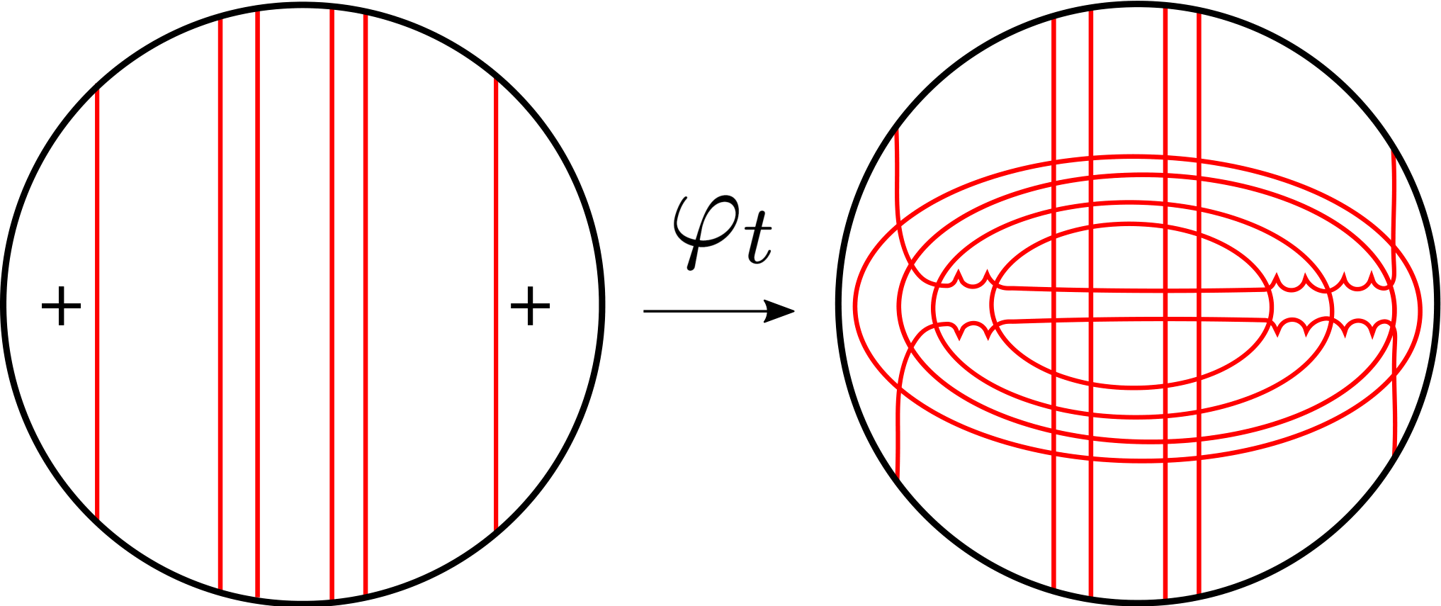
Refer to caption
Figure 38. Description of the homotopy φt\varphi_{t}. Observe that the cusp points appear in pairs, therefore no zeroes of the area function appear.
Proof.

Denote the two curves of strict Legendrian immersions in 𝔻G=πG∘φ⁡(𝔻){\mathbb{D}}_{G}=\pi_{G}\circ\varphi({\mathbb{D}}) by C0C_{0} and C1C_{1}. Let i∈{0,1}i\in\{0,1\} and fix γi∈Ci\gamma^{i}\in C_{i}. Choose a path γs\gamma^{s}, s∈[−1,2]s\in[-1,2], transversal to the strict immersions curves at CiC_{i} such that Ci∩{γs:s∈[−1,2]}={γi}C_{i}\cap\{\gamma^{s}:s\in[-1,2]\}=\{\gamma^{i}\}. A neighborhood K={γrs:s∈[−1,2],r∈[−1,1]}⊆𝔻K=\{\gamma^{s}_{r}:s\in[-1,2],r\in[-1,1]\}\subseteq{\mathbb{D}} of the path γs\gamma^{s} may be assumed to satisfy γrs≡γs\gamma^{s}_{r}\equiv\gamma^{s} for s∈[−1,2]s\in[-1,2].

Apply Proposition 8.1.15 to find a disk E={γs,u:s,u∈[0,1]}E=\{\gamma^{s,u}:s,u\in[0,1]\} such that

  • •

    γs,0=γs\gamma^{s,0}=\gamma^{s}, s∈[0,1]s\in[0,1].

  • •

    C={γs,u∈𝔏​𝔢​𝔤​ℑ​𝔪​𝔪strict​(ℝ3):(s,u)∈{0,1}×[0,1]∪[0,1]×{1}}C=\{\gamma^{s,u}\in{\mathfrak{LegImm}^{\textbf{strict}}}({\mathbb{R}}^{3}):(s,u)\in\{0,1\}\times[0,1]\cup[0,1]\times\{1\}\} is a continuous curve of strict Legendrian immersions, with self-intersection times t0s,u,t1s,u∈𝕊1t_{0}^{s,u},t_{1}^{s,u}\in{\mathbb{S}}^{1}, t0s,u≠t1s,ut_{0}^{s,u}\neq t_{1}^{s,u}.

  • •

    𝒮j={γsj,u:u∈[0,1]\mathcal{S}_{j}=\{\gamma^{s_{j},u}:u\in[0,1], j∈{1,…,ν}j\in\{1,\ldots,\nu\}, is a curve of strict Legendrian immersions,

  • •

    There is a finite number of curves 𝒞n\mathcal{C}_{n} of strict Legendrian immersions defined by

    𝒞n={γs,u:(s,u)∈[0,1]×{un}},\mathcal{C}_{n}=\{\gamma^{s,u}:(s,u)\in[0,1]\times\{u_{n}\}\},

    where 0<u1<⋯<un<10<u_{1}<\cdots<u_{n}<1. The self-intersection times of γs,un\gamma^{s,u_{n}} are τ0s,un,τ1s,un∈𝕊1\tau_{0}^{s,u_{n}},\tau_{1}^{s,u_{n}}\in{\mathbb{S}}^{1}, with τ0s,un≠τ1s,un\tau_{0}^{s,u_{n}}\neq\tau_{1}^{s,u_{n}}. These curves do not have cusp points.

  • •

    τis,un≠tjs,un\tau_{i}^{s,u_{n}}\neq t_{j}^{s,u_{n}}, for each i,j∈{0,1}i,j\in\{0,1\} and (s,un)∈C∩𝒞n(s,u_{n})\in C\cap\mathcal{C}_{n}.

Apply Lemma 7.2.1 to lift EE into a disk of horizontal immersions. Now, apply again Lemma 7.2.1 over CC in t0s,u−εt_{0}^{s,u}-\varepsilon and t0s,u+εt_{0}^{s,u}+\varepsilon, for ε>0\varepsilon>0 small enough in order to increase the area function at will. Do likewise over the self–intersection points in 𝒞n\mathcal{C}_{n}. Note that there is no interaction between the two deformations because the self–intersection times are different.

By construction the outward normal vector field XX to C=∂EC=\partial E coincides with the standard orientation. Push CC in the direction of XX to obtain an extended disk E~={γs,u:s∈[−1,2],u∈[0,2]}⊇E\tilde{E}=\{\gamma^{s,u}:s\in[-1,2],u\in[0,2]\}\supseteq E in 𝔏​𝔢​𝔤​ℑ​𝔪​𝔪​(ℝ3){\mathfrak{LegImm}}({\mathbb{R}}^{3}), which lifts to ℌ​𝔬​𝔯​(ℝ4){\mathfrak{Hor}}({\mathbb{R}}^{4}), such that γs,0=γs\gamma^{s,0}=\gamma^{s} for each s∈[−1,2]s\in[-1,2]. We define the map

ψ:[−1,2]×[0,2]×[−1,1]→ℌ​𝔬​𝔯​(ℝ4):(s,u,r)↦γrs,u=γs,u.\psi:[-1,2]\times[0,2]\times[-1,1]\to{\mathfrak{Hor}}({\mathbb{R}}^{4}):(s,u,r)\mapsto\gamma^{s,u}_{r}=\gamma^{s,u}.

See Figure 39, to visualize the piecewise linear disk that we are about to define in [−1,2]×[0,2]×[−1,1]⊆ℝ3[-1,2]\times[0,2]\times[-1,1]\subseteq{\mathbb{R}}^{3}. First, we define the base (a closed piecewise linear curve in ℝ2{\mathbb{R}}^{2}):

ΔB={(s,r)∈[−1,2]×[−1,1]:|r|≤g⁡(s)},\Delta_{B}=\{(s,r)\in[-1,2]\times[-1,1]:|r|\leq g(s)\},

for

g⁡(s)={1+s,if ​s∈[−1,0],1,if ​s∈[0,1],2−s,if ​s∈[1,2].g(s)=\left\{\begin{array}[]{cc}1+s,&\text{if }s\in[-1,0],\\ 1,&\text{if }s\in[0,1],\\ 2-s,&\text{if }s\in[1,2].\end{array}\right.

And now the piecewise linear graph in ℝ3{\mathbb{R}}^{3} as

Δ={(s,u,r)∈[−1,2]×[1,2]×[−1,1]:(s,r)∈ΔB,u={2+s−|r|,if ​s∈[−1,0],2−|r|,if ​s∈[0,1],3−s−|r|,if ​s∈[1,2].}.\Delta=\left\{(s,u,r)\in[-1,2]\times[1,2]\times[-1,1]:(s,r)\in\Delta_{B},u=\left\{\begin{array}[]{cc}2+s-|r|,&\text{if }s\in[-1,0],\\ 2-|r|,&\text{if }s\in[0,1],\\ 3-s-|r|,&\text{if }s\in[1,2].\end{array}\right.\right\}.
Refer to caption
Figure 39. Construction of 𝔻~\tilde{{\mathbb{D}}}.

We define a new (piecewise linear) disk Δ^=(∂(ΔB)×[0,1])∪Δ⊆[−1,2]×[0,2]×[−1,1]\hat{\Delta}=(\partial(\Delta_{B})\times[0,1])\cup\Delta\subseteq[-1,2]\times[0,2]\times[-1,1]. Observe that the boundary of Δ^\hat{\Delta} coincides with ∂ΔB\partial\Delta_{B}, therefore we can define a new disk 𝔻~=(𝔻∖ΔB)∪Δ^\tilde{{\mathbb{D}}}=({\mathbb{D}}\setminus\Delta_{B})\cup\hat{\Delta} gluing along the boundaries. We can define a new morphism

φ1:𝔻~\displaystyle\varphi_{1}:\tilde{{\mathbb{D}}} →\displaystyle\to ℌ​𝔬​𝔯​(ℝ4)\displaystyle{\mathfrak{Hor}}({\mathbb{R}}^{4})
p\displaystyle p ↦\displaystyle\mapsto {φ0​(p),p∈(𝔻∖ΔB),ψ⁡(p),p∈Δ^.\displaystyle\left\{\begin{array}[]{cc}\varphi_{0}(p),&p\in({\mathbb{D}}\setminus\Delta_{B}),\\ \psi(p),&p\in\hat{\Delta}.\end{array}\right.

It is left to check that φ0\varphi_{0} and φ1\varphi_{1} are homotopic. This is performed by building any homotopy between the two disks ΔB\Delta_{B} and Δ^\hat{\Delta} relative to the boundary ∂ΔB\partial\Delta_{B} inside [−1,2]×[0,2]×[−1,1][-1,2]\times[0,2]\times[-1,1]. ∎

8.2. Globalization.

We use the theory developed in the last two Subsections to prove the main theorem of Section 7. We first adapt a previous construction.

Lemma 8.2.1.

[Corollary of Lemma 8.1.19]

Let φ:𝔻⁡(x,y)→ℌ​𝔬​𝔯​ℑ​𝔪​𝔪​(ℝ4)\varphi:{\mathbb{D}}(x,y)\rightarrow{\mathfrak{HorImm}}({\mathbb{R}}^{4}) be a disk of horizontal immersions such that:

  • (i)

    φ⁡(∂𝔻)⊆ℌ​𝔬​𝔯​(ℝ4)\varphi(\partial{\mathbb{D}})\subseteq{\mathfrak{Hor}}({\mathbb{R}}^{4}),

  • (ii)

    (πG∘φ)−1​(𝔏​𝔢​𝔤​ℑ​𝔪​𝔪strict​(ℝ3))=C(\pi_{G}\circ\varphi)^{-1}({\mathfrak{LegImm}^{\textbf{strict}}}({\mathbb{R}}^{3}))=C is a connected curve with a unique zero of the area function β∈C\beta\in C.

Then, there exists a 11–parametric family of disks φt:𝔻→ℌ​𝔬​𝔯​ℑ​𝔪​𝔪​(ℝ4)\varphi^{t}:{\mathbb{D}}\rightarrow{\mathfrak{HorImm}}({\mathbb{R}}^{4}), t∈[0,1]t\in[0,1], satisfying

  • (i)

    φ0=φ\varphi^{0}=\varphi,

  • (ii)

    φt|∂𝔻=φ0|∂𝔻\varphi^{t}_{|\partial{\mathbb{D}}}=\varphi^{0}_{|\partial{\mathbb{D}}},

  • (iii)

    there is a C0C^{0} deformation CtC_{t}, t∈[0,1]t\in[0,1], of C=C0C=C_{0} and a family of connected curves StS_{t} such that

    • –

      (πG∘φt)−1​(𝔏​𝔢​𝔤​ℑ​𝔪​𝔪strict​(ℝ3))=Ct∪St(\pi_{G}\circ\varphi^{t})^{-1}({\mathfrak{LegImm}^{\textbf{strict}}}({\mathbb{R}}^{3}))=C_{t}\cup S_{t},

    • –

      β∈Ct\beta\in C_{t} is the unique zero of the area function in φt\varphi^{t} and the curves StS_{t} encircle β\beta,

    • –

      Ct=C0C_{t}=C_{0} for t∈[0,1/2)t\in[0,1/2),

    • –

      C1C_{1} is a DS of C1/2C_{1/2} in the moduli (see Lemma 8.1.19) and β\beta lies between the first and the second cusp.

    • –

      St=∅S_{t}=\emptyset for t∈[0,1/2)t\in[0,1/2),

    • –

      St={x2+y2=(12−t)2}S_{t}=\{x^{2}+y^{2}=(\frac{1}{2}-t)^{2}\} for t∈[1/2,3/4]t\in[1/2,3/4] and

    • –

      St=S3/4S_{t}=S_{3/4} for t∈[3/4,1]t\in[3/4,1].

See Figure 40.

Proof.
Figure 40. Schematic description of Lemma 8.2.1. The blue point in the middle of the circle represents β\beta and the red middle circle in the cylinder the self–intersection (with non zero area) created in the DS.

Since the problem is local we may assume that the disk is small and the self–intersection times for the Legendrian projections in the curve CC are constant and equal to t0t_{0} and t1t_{1}. Choose t2∈𝕊1t_{2}\in{\mathbb{S}}^{1} a time value different from t0t_{0} and t1t_{1}. Use polar coordinates 𝔻=𝔻⁡(r,θ){\mathbb{D}}={\mathbb{D}}(r,\theta) and define parametrically for each horizontal immersion φ⁡(r,θ)\varphi(r,\theta) a DS that is denoted B=𝔻×[0,1/2]→ℌ​𝔬​𝔯​ℑ​𝔪​𝔪​(ℝ4)B={\mathbb{D}}\times[0,1/2]\to{\mathfrak{HorImm}}({\mathbb{R}}^{4}), where B⁡(r,θ,h)B(r,\theta,h), h∈[0,1/2]h\in[0,1/2], is the DS of φ⁡(r,θ)\varphi(r,\theta).

Now we apply Lemma 8.1.19 in order to further deform and create 44 cusp points in the moduli: just sliding one branch (t0t_{0}) over the other (t1t_{1}). Apply Lemma 7.2.1 to place the zero in the required position. This second deformation produces a family of disks B⁡(r,θ,h)B(r,\theta,h) with h∈[1/2,1]h\in[1/2,1].

Define

L={B(r,θ,h):r=12,h∈[0,1]}⊆Image(B),L=\{B(r,\theta,h):\,r=\frac{1}{2},h\in[0,1]\}\subseteq{\operatorname{Image}}(B),
T=𝔻(r≤12)×{h=1}⊆Image(B),T={\mathbb{D}}\left(r\leq\frac{1}{2}\right)\times\{h=1\}\subseteq{\operatorname{Image}}(B),

that builds a piecewise linear disk 𝔻′=L∪T{\mathbb{D}}^{\prime}=L\cup T whose boundary coincides with the boundary of 𝔻⁡(r≤12)⊆𝔻{\mathbb{D}}(r\leq\frac{1}{2})\subseteq{\mathbb{D}}. Replace 𝔻⁡(r≤12){\mathbb{D}}(r\leq\frac{1}{2}) by 𝔻′{\mathbb{D}}^{\prime}, ie define 𝔻~=(𝔻∖𝔻⁡(r≤12))∪𝔻′\tilde{\mathbb{D}}=({\mathbb{D}}\setminus{\mathbb{D}}(r\leq\frac{1}{2}))\cup{\mathbb{D}}^{\prime}. The associated diagram of strict immersions conforms the statement of the Lemma. See Figure 40. ∎

Proof of Theorem 7.1.2.

Let γθ\gamma^{\theta} be a loop of horizontal embeddings which lies in π1​(ℌ​𝔬​𝔯​(ℝ4))0\pi_{1}({\mathfrak{Hor}}({\mathbb{R}}^{4}))_{0}, ie RotL⁡(γθ)=0\operatorname{Rot}_{L}(\gamma^{\theta})=0. Assume that Area⁡(γθ)=0\operatorname{Area}(\gamma^{\theta})=0, we must check that γθ\gamma^{\theta} is trivial.

Let 𝔻{\mathbb{D}} be a disk in ℌ​𝔬​𝔯​ℑ​𝔪​𝔪​(ℝ4){\mathfrak{HorImm}}({\mathbb{R}}^{4}) whose boundary is given by {γθ}\{\gamma^{\theta}\}. Apply successively Proposition 7.3.1 to assume that each curve of strict Legendrian immersions in 𝔻G{\mathbb{D}}_{G} has at most one zero of the area function. Since Area⁡(γθ)=0\operatorname{Area}(\gamma^{\theta})=0 the number of zeroes is even. If 𝔻G{\mathbb{D}}_{G} has not zeroes then we are done. Hence, assume that 𝔻G{\mathbb{D}}_{G} has a positive number of zeroes and denote them β0,…,β2​n−1\beta_{0},\ldots,\beta_{2n-1}.

Let Ck⊆𝔻GC_{k}\subseteq{\mathbb{D}}_{G} be the curve of strict Legendrian immersions that contains βk\beta_{k}, k∈{0,…,2​n−1}k\in\{0,\ldots,2n-1\}. It is sufficient to show that we can do a surgery along any two curves C0C_{0} and C1C_{1} to produce a new curve of strict Legendrian immersions that contains the zeroes β0\beta_{0} and β1\beta_{1} without creating any new zero. Application of Proposition 7.3.1 will provide the required result.

To formalize the previous discussion, note that CiC_{i} is naturally oriented by the gradient vector gig_{i} of the Area function at βi\beta_{i}. Together with the standard co-orientation of Σ1,0\Sigma^{1,0} at βi\beta_{i}, denoted by wiw_{i}, it provides an oriented basis at Tβi​𝔻T_{\beta_{i}}{\mathbb{D}} namely {gi,wi}\{g_{i},w_{i}\}. We can assume that the orientations induced at the two points β0\beta_{0} and β1\beta_{1} are the same. If it is not the case, apply Lemma 8.2.1 in order to change the orientation of the curve C0C_{0}. This works because the Area function changes signs when crossing a cusp in the curve C0C_{0} and thus the gradient of the area function over the zero gets multiplied by −1-1.

Select a pair of points αi\alpha_{i} arbitrarily close to βi\beta_{i}, whose area function is positive. Fix an embedded curve α:[0,1]→𝔻\alpha:[0,1]\to{\mathbb{D}} such that α⁡(i)=αi\alpha(i)=\alpha_{i} and it is transverse to CiC_{i}. Moreover, we assume that d​αtd​t|t=0\frac{d\alpha_{t}}{dt}_{|t=0} defines the standard coorientation at α0∈Σ1,0\alpha_{0}\in\Sigma^{1,0}. Respectively d​αtd​t|t=1\frac{d\alpha_{t}}{dt}_{|t=1} defines the opposite orientation to the standard one (see Figure 41 to learn how to deal with the wrong coorientation case).

Figure 41. Embedded path connecting α0\alpha_{0} and α1\alpha_{1} conforming to the coorientations rule.

A small tubular neighborhood 𝔻α{\mathbb{D}}_{\alpha} of the path satisfies the hypothesis of Proposition 8.1.22. This implies that we can get a deformed disk with the same number of zeroes such that the deformation is performed compactly supported on the disk 𝔻α{\mathbb{D}}_{\alpha} following the Diagram explained in Figure 38. This new diagram makes the two zeroes βi\beta_{i} be part of the same connected component of curves of strict immersions, see Figure 42. This is ensured by the compatibility of the orientations that we have enforced in the basis {gi,wi}\{g_{i},w_{i}\} of Tβi​𝔻T_{\beta_{i}}{\mathbb{D}}. Apply Proposition 7.3.1 to cancel the two zeroes.

Refer to caption
Figure 42. Schematic description of the neighborhood of α⁡(t)\alpha(t). The cusps between the concentric circles are not drawn to make the picture easier to understand.

∎

References

  • [1] J. Adachi. Classification of horizontal loops in standard Engel space. Int. Math. Res. Not. 2007; Vol. 2007: article ID rnm008, 29 pages, doi:10.1093/imrn/rnm008.
  • [2] C. C. Adams. The knot book. An elementary introduction to the mathematical theory of knots. American Mathematical Society, Providence, RI, 2004. xiv+307 pp.
  • [3] V. I. Arnold, S. M. Gusein-Zade, A. N. Varchenko. Singularities of Differentiable Maps. Volume I. Birkhäuser, Boston, Basel, Sttutgart. 1985.
  • [4] D. Bennequin. Entrelacements et équations de Pfaff. Third Schnepfenried geometry conference, Vol. 1 (Schnepfenried, 1982), 87–161, Astérisque, 107-108, Soc. Math. France, Paris, 1983.
  • [5] R. Budney. A family of embedding spaces. Geometry & Topology 13 (2008): 41–83.
  • [6] R. Casals, A. del Pino. Classification of Engel knots. arXiv:1710.11034.
  • [7] Y. Chekanov. Differential algebra of Legendrian links. Invent. Math. 150 (2002), no. 3, 441–483.
  • [8] F. Ding, H. Geiges. The diffeotopy group of 𝕊1×𝕊2{\mathbb{S}}^{1}\times{\mathbb{S}}^{2} via contact topology. Compos. Math. 146 (2010), no. 4, 1096?1112.
  • [9] Y. Eliashberg. Classification of contact structures on ℝ3{\mathbb{R}}^{3}. Internat. Math. Res. Notices 1993, no. 3, 87–91.
  • [10] Y. Eliashberg, M. Fraser. Topologically trivial Legendrian knots. J. Symplectic Geom. 7 (2009), no. 2, 77–127.
  • [11] Y. Eliashberg, N. Mishachev, Introduction to the hh–Principle. Graduated Studies in Mathematics, 48. AMS, Providence, RI, 2002.
  • [12] J. Etnyre. Legendrian and transversal knots. Handbook of knot theory, 105–185, Elsevier B. V., Amsterdam, 2005.
  • [13] J. Etnyre and K. Honda. Knots and contact geometry I: Torus knots and the figure eight knot. J. Symplectic Geom. 1 (2001), 63-120.
  • [14] D. Fuchs, S. Tabachnikov. Invariants of Legendrian and transverse knots in the standard contact space. Topology 36 (1997), no. 5, 1025–1053.
  • [15] H. Geiges. An Introduction to Contact Topology. Cambr. Studies in Adv. Math. 109. Cambr. Univ. Press 2008.
  • [16] H. Geiges. Horizontal loops in Engel space. Math. Ann. Oct 2008, Vol. 342, no. 2, 291–296.
  • [17] R. S. Hamilton. The inverse function theorem of Nash and Moser. Bull. Amer. Math. Soc. (N.S.) 7 (1982), no. 1, 65–222.
  • [18] A. Hatcher. A proof of the Smale conjecture, Diff⁡(𝕊3)≃O⁡(4){\rm Diff({\mathbb{S}}^{3})}\simeq O(4). Ann. of Math. (2) 117 (1983), no. 3, 553–607.
  • [19] A. Hatcher, Algebraic topology. Cambridge University Press, Cambridge, 2002. xii+544 pp. ISBN: 0-521-79160-X; 0-521-79540-0
  • [20] A. Hatcher. Spaces of knots. arXiv:math/9909095.
  • [21] M.W. Hirsch. Immersions of manifolds. Trans. Amer. Math. Soc. 93 1959 242–276.
  • [22] K. Igusa. Higher singularities of smooth functions are unnecessary. Ann. of Math. (2) 119 (1984), no. 1, 1?58.
  • [23] T. Kálmán. Contact homology and one parameter families of Legendrian knots. Geometry & Topology 9 (2005): 2013–2078.
  • [24] S. Lang, Fundamentals of differential geometry. Graduate Texts in Mathematics, 191. Springer-Verlag, New York, 1999. xviii+535 pp. ISBN: 0-387-98593-X 53-01 (58-01)
  • [25] L. Ng. Computable Legendrian invariants. Topology 42 (2003), no. 1, 55–82.
  • [26] J. Milnor. Morse theory. Based on lecture notes by M. Spivak and R. Wells. Annals of Mathematics Studies, No. 51 Princeton University Press, Princeton, N.J. 1963 vi+153 pp. 57.50 (53.72)
  • [27] A. del Pino, F. Presas. Flexibility for tangent and transverse immersions in Engel manifolds. arXiv:1609.09306.
  • [28] J. M. Sabloff, M. G. Sullivan. Families of Legendrian submanifolds via generating families. Quantum Topol. 7 (2016), no. 4, 639–668.
  • [29] P. Ozsváth, Z. Szabó, D. Thurston. Legendrian knots, transverse knots and combinatorial Floer homology. Geometry & Topology 12 (2008), no. 2, 941–980.