Analysis and Synthesis of MIMO Multi-Agent Systems Using Network Optimization
Abstract
This work studies analysis and synthesis problems for diffusively coupled multi-agent systems. We focus on networks comprised of multi-input multi-output nonlinear systems that posses a property we term maximal equilibrium-independent cyclically monotone passivity (MEICMP), which is an extension of recent passivity results. We demonstrate that networks comprised of MEICMP systems are related to a pair of dual network optimization problems. In particular, we show that the steady-state behavior of the multi-agent system correspond to the minimizers of appropriately defined network optimization problems. This optimization perspective leads to a synthesis procedure for designing the network controllers to achieve a desired output. We provide detailed examples of networked systems satisfying these properties and demonstrate the results for a network of damped planar oscillators.
I Introduction and Motivation
Multi-agent systems have been extensively studied in recent years, mainly due to their applications in various fields in the sciences and engineering, e.g. robotics, neural networks, and power grids [1, 2, 3]. The study of graphs and their algebraic representations have emerged as an important tool in the modeling and analysis of these systems [4]. When the agents are considered as dynamical systems, then the notion of passivity theory brings a powerful framework to analyze the dynamic behavior of these interconnected systems. Passivity theory enables an analysis of the networked system that decouples the dynamics of the agents in the ensemble, the structure of the information exchange network, and the protocols used to couple interacting agents [5]. Passivity for multi-agent systems was first pursued in [6], where it was used to study group coordination problems. Several variants of passivity theory were used in various contexts like coordinated control of robotic systems [7], synchronization problems [8, 9], port-Hamiltonian systems on graphs [10], and distributed optimization [11].
One important variant of passivity particularly useful for the analysis of multi-agent systems is equilibrium-independent passivity (EIP), introduced in [12]. For EIP systems, passivity is verified with respect to any steady-state input-output pair, allowing one to show convergence results without specifying the limit beforehand [13]. A generalization of this result known as maximal monotone equilibrium-independent passivity (MEIP) was introduced in [14] for SISO systems, allowing to prove convergence using energy methods for a much wider class of systems, including, for example, integrators, that are not EIP.
These passivity extensions have proved very powerful in the analysis of networked systems. Of interest to this work, [14] used the MEIP notion to establish an equivalence between the steady-state behavior of networked systems and the solution of a pair of dual network optimization problems. Thus, the analysis of networks comprised of MEIP passive agents and controllers could be accomplished by studying an associated static optimization problem. These results were recently extended in [15] to provide a synthesis procedure for the interaction protocols between agents to enforce a desired relative state configuration between the agents. In [16], an equivalence between feedback passivation of passivity short systems was made with a regularization of the corresponding network optimization problems.
The main shortcoming of these works building upon MEIP systems is that they are only applicable to single-input single-output (SISO) agents; this is a consequence of the monotonicity requirement of the steady-state input-output relations that cannot be easily generalized to systems with more than one input or output. This shortcoming motivates the current work, where we aim to extend the notion of MEIP passivity for both the analysis and synthesis of networked systems comprised of multi-input multi-output (MIMO) systems.
The main analytic tool required to study MIMO systems in this context is the notion of cyclically monotone (CM) relations, originally introduced in [17]. Cyclically monotone relations provide the correct generalization of monotonicity of scalar functions to vector functions. The key result due to [17] shows that CM relations are contained in the sub-gradient of a convex function. With this tool in hand, we are able to extend the SISO results from [14] to square MIMO systems. The main contributions of this work can now be stated as follows:
- •
We develop a MIMO counterpart of monotone equilibrium independent passivity using the notion of cyclically monotone relations, which we term maximal equilibrium-independent cyclically monotone passivity (MEICMP).
- •
We show that a diffusively coupled network comprised of MIMO systems that are (output-strictly) MEICMP with controllers that are also MEICMP converge to an output agreement steady-state. Moreover, we show that the steady-states of the system are the optimal solutions of a dual pair of network optimization problems.
- •
We propose a synthesis procedure for designing network controllers assuring global asymptotic convergence to a desired output. We present conditions for when such a synthesis is feasible. If a synthesis is not feasible, we present a practically-justifiable method for plant augmentation assuring the synthesis problem can be solved for any desired steady-state output.
We also provide numerous examples of systems that can be classified as MEICMP including convex-gradient dynamical systems with oscillatory terms and damped oscillators.
The remainder of the paper is organized as follows. Section II reviews the network model and results on passivity in multi-agent coordination. In Section III, we present the main results in three subsections. The first studies steady-states of the closed loop system. The second introduces the notion of cyclically monotone relations and shows how they can be understood via network optimization problems. The third shows that if the agents and the controllers are all assumed to be MEICMP, then the closed-loop system converges to the steady-states. The remaining subsections provide analysis results for networks comprised of MEICMP systems and their relation to a class of dual network optimization problems. Section IV deals with the synthesis problem, providing a characterization for solvable cases and a corresponding synthesis procedure. Section V presents examples of systems with cyclically monotone input-output relations.
Preliminaries
A graph consists of a node set and edge set . Each edge consists of two vertices , and we orient it arbitrarily, say from to ; we write in this case. We define the incidence matrix of as a matrix such that for any edge , and all other entries in ’s column are zero. Given some integer , thought of as the input- and output- dimensions of the dynamical system of each of the agents, we define the incidence operator as , where is the identity operator and is the Kronecker product. It is important to note that the null-space of consists of all vectors of the form . Also, if is a convex function, its Legendre transform is defined as by [18]. Furthermore, consider the indicator function for the set , denoted , defined by whenever , and otherwise. Of particular interest is when the set , and we denote the indicator function in that case as . For a map , we denote its image by . If is a linear map, the kernel of is denoted by . From now on, we will use italicized letters (e.g., or ) to denote time-dependent signals, and normal font letters (e.g. ) to denote constant vectors. Finally, for sets , we define .
II Diffusively Coupled Networks and the
Role of Passivity in Cooperative Control
In this section, we introduce the network dynamic model used in this work and present an overview of the role of passivity in cooperative control.
II-A The Diffusively Coupled Network Model
We consider a population of agents that interact over a network, described by the graph . The agents are represented by the vertices , and pairs of interacting agents are represented by edges . Each specific edge contains information about the coupling (i.e., the controllers), which are allowed to be dynamic. We assume a diffusive coupling structure, where the input to the edge controllers are the difference between the output of the adjacent agents, and the control input of each agent is the (directed) sum of the edge controller outputs.
Each agent in the network is modeled as a square multiple-input multiple-output dynamic system of the form
| (1) |
where is the state, the input, the output, and a constant exogenous input. Note that each agent need not have the same state dimension, but we require all agents have the same number of inputs and outputs (). Let and be the concatenation of the input and output vectors. Similarly, is the stacked state vector, and the stacked exogenous input.
The agents are diffusively coupled over the network also by a dynamic system that we consider as the network controllers. For the edge , we denote the difference between the output of the adjacent nodes as . The stacked vector can be compactly expressed using the incidence operator of the graph as . These, in turn, drive the edge controllers described by the dynamics
| (2) |
The output of these controllers will yield an input to the node dynamical systems as , with the stacked vector of controller outputs. We denote the complete network system by the triple , where and are the parallel interconnection of the agent and controller systems, and the underlying network; see Figure 1.
II-B The Role of Passivity in Cooperative Control
Passivity theory has taken an outstanding role in the analysis of cooperative control systems, and in particular those with the diffusive coupling structure of Figure 1. We dedicate this section to consider a few variants of passivity used to prove various analysis results for multi-agent systems. The main advantage of using passivity theory is that it allows to decouple the system into three different layers - namely the agent dynamics, the coupling dynamics, and the network connecting the two. This concept is clearly seen in the following theorem:
Theorem 1 ([14]).
Consider the network system comprised of agents and controllers. Suppose that there are constant vectors and such that
- i)
the systems are output strictly-passive with respect to and ;
- ii)
the systems are passive with respect to and ;
- iii)
the stacked vectors and satisfy and .
Then the output vector converges to as .
Indeed, the first condition involves the agent dynanics, the second the controllers, and the third the underlying network.
The first paper to fully embrace passivity theory to analyse cooperative control problems was [6]. This led to many variants of passivity in the literature proven to be useful for the analysis of cooperative control problems. Incremental passivity (IP), introduced in [19], allows one to consider the passivity property with respect to certain trajectories, rather than fixed equilibria. Indeed, incremental passivity was used in [8, 9] to prove various synchronization and analysis results in multi-agent system. However, IP is restrictive, as it demands the passivation inequality to hold for any two trajectories.
Other variants of passivity focus on the collection of all equilibria of a system. In this direction, the notion of steady-state input-output maps is useful. In the following, we focus on dynamical systems of the form
| (3) |
Definition 1.
With this definition, we now introduce the next variant of passivity termed equilibrium-independent passivity (EIP) [12]. A key feature of EIP is the assumption that for any steady-state input there is exactly one steady-state output . This implies that the steady-state output can be expressed as a continuous function of the steady-state input . Thus, with a slight abuse of notation we can consider the the set as a function , i.e. . In general, this is less restrictive than IP, and allows to prove analysis results for MIMO systems. However, there are IP systems which are not EIP. The epitome of these kind of systems is the simple integrator, which can be verified to be IP, but not EIP. The steady-state input has multiple different steady-state outputs (depending on the initial condition of the system), and thus the input-output map is no longer a function.
The last variant of passivity we review is maximal equilibrium-independent passivity (MEIP) [14]. It is a variant of EIP that attempts to remedy the exclusiveness of the simple integrator and similar systems. However, it is only defined in the case of SISO systems, as it relies on the notion of monotone relations:
Definition 2 ([14]).
Consider a relation . We say that is a monotone relation if for every two elements and , we have that . We say that is maximally monotone if it is monotone and is not contained in a larger monotone relation.
In other words, increasing the first element implies that the second element cannot decrease. We now present the definition of MEIP.
Definition 3 ([14]).
The SISO system (3) is said to be maximal equilibrium-independent passive (MEIP) if:
- i)
The system is passive with respect to any steady-state pair it has.
- ii)
The collection of all steady-state input-output pairs is maximally monotone.
This is indeed a generalization of EIP, as the function of an EIP system is monotone ascending [12]. It can also be shown that the simple SISO integrator is MEIP. However, the problem of finding a MIMO analogue of MEIP, or a variant of EIP that will include marginally-stable systems like the simple integrator, has not been addressed in the literature.
In the following section, we present a generalization of MEIP and of EIP to MIMO systems which include integrators and other marginally-stable systems. The key notion that we’ll use is one possible generalization of monotonic relations from subsets of to subsets of . This generalization is called cyclic monotonicity, and was first considered in [17].
III Cyclically Monotone Relations
and Cooperative Control
In [14], the concept of monotone relations is used to provide convergence results for a network system comprised of SISO agents. However, many applications deal with MIMO systems, necessitating a need to extend this work for network systems consisting of MIMO agents. We begin by considering the steady-states of the system.
III-A Steady-States and Network Consistency
Consider a steady-state of the closed loop system in Fig. 1. We know that for every , is a steady-state input-output pair of the -th agent . Similarly, for every , is a steady-state input-output pair of the -th controller . The network interconnection between the systems and imposes an additional consistency constraint between these steady-state values. This motivates us to consider the steady-state input-output relations for each of the agents and the controllers.
In this direction, we denote the steady-state input-output relation of the -th agent by , and the relation for the -th controller by . That is, and . We denote the stacked relation for the agents and controllers as and , respectively.
Remark 1.
Suppose that is a steady-state input-output relation. We can consider a set-valued map, also denoted by , taking a steady-state input to the set . Similarly, one can consider the inverse set-valued map taking a steady-state output to the set . Thus, with a slight abuse of notation we refer to () as both a relation and a set-valued map.
Proposition 1.
Let be any four constant vectors. Then is a steady-state of the closed-loop system if and only if
| (4) |
Proof.
Follows directly from the interconnection of the network, and from the definitions of and . ∎
We wish to manipulate the conditions in (4) to reduce the steady-state characterization from a system with four constraints to one.
Proposition 2.
Let be any vector. Then the following conditions are equivalent:
- i)
The zero vector belongs to the set .
- i)
There exists vectors such that is a steady-state of the closed-loop network .
Proof.
By the same methods, we can also reduce the conditions (4) to an inclusion in the edge-variables .
Proposition 3.
Let be any vector. Then the following conditions are equivalent:
- i)
The zero vector belongs to the set .
- ii)
There exists vectors such that is a steady-state of the closed-loop network .
Proof.
Same as the proof of Proposition 2. ∎
III-B Connecting Steady-States to Network Optimization
So far, we showed that the steady-states of the closed-loop system can be understood using the following two conditions:
| (5) |
However, these conditions are highly nonlinear, and would be difficult to solve even if they were equations instead of inclusions. One method of dealing with nonlinear equations of the form for some function , is to consider its integral function instead. Suppose there is a function such that . In that case, we can find a solution to by solving the unconstrained minimization problem . If, in addition, the function is convex, the solution to the minimization problem can often be computed efficiently (i.e. in polynomial time).
In general, convex functions need not be smooth, or even differentiable. In this case, the notion of the subdifferential of a convex function can be employed. The subdifferential of the convex function at the point is denoted , and consists of all vectors such that
See [20] for more on subdifferentials. Note that the subdifferential is a set-valued map. Also, analogously to the differentiable case, is a minimum point of if and only if . Thus, if we are able to require that and are gradients of convex functions (i.e., their integral functions are convex), then the nonlinear inclusions in (5) may be solved using convex optimization. In fact, these functions have been characterized due to Rockafellar [17]:
Definition 4 (Cyclic Monotonicity).
Let be an integer, and consider a subset of . We say that is a cyclically monotonic (CM) relation if for any and any pairs of -vectors, the following inequality holds,
| (6) |
Here, we use the convention that . We say that is strictly cyclically monotonic (SCM) if the inequality (6) is sharp whenever at least two ’s are distinct. We term the relation as maximal CM (or maximal SCM) if it is not strictly contained in a larger CM (SCM) relation.
This is a generalization of the concept of monotone relations for SISO system, which we elaborate upon later.
Theorem 2 ([17]).
A relation is the subgradient of a convex function if and only if it is maximal CM. Moreover, it is the sub-gradient of a strictly convex function if and only if it is maximal SCM. The convex function is unique up to an additive scalar.
Remark 2.
If is maximally CM, and is a convex function such that , then is the integral function of .
Rockafellar’s Theorem gives us a way to check that a relation is the subdifferential of a convex function. If we want to state the conditions in (5) as the solutions of convex minimization problems, we need to assume that the input-output relations appearing are CM. This, together with (1), motivates the following system-theoretic definition:
Definition 5.
A system is maximal equilibrium-independent cyclically monotone (output strictly) passive (MEICMP) if
- i)
for every steady-state input-output pair , the system is (output strictly) passive with respect to and ;
- ii)
the set of all steady-state input-output pairs, , is maximally (strictly) cyclically monotonic.
If is strictly cyclically monotone, we say that is maximal equilibrium-independent strictly cyclically monotone (output strictly) passive (MEISCMP).
Remark 3.
It can be shown that when , a relation is cyclically monotone if and only if it is monotone. Thus, a SISO system is MEIP if and only if it is MEICMP [20].
Now, suppose that the agents and the controllers are all MEICMP with steady-state input maps and . We let and be the associated integral functions, which as a result of Theorem 2, are convex functions. We let and be their sum, so that and . As these are convex functions, we can look at the dual convex functions and , namely
and similarly for [20]. These are convex functions that satisfy and [20]. The functions allows us to convert the conditions (5) to the unconstrained minimization problems of and . Recalling that and that , we can state the minimization problems in the following form:
| Optimal Potential Problem | Optimal Flow Problem |
|---|---|
| (OPP) | (OFP) |
These static optimization problems, known as the Optimal Potential Problem and Optimal Flow Problem, are two fundamental problems in the field of network optimization, which has been widely studied in computer science, mathematics, and operations research for many years [20]. A well-known instance of these problems is the maximum-flow/minimum-cut problems, which are widely used by algorithmists and by supply chain designers [21].
We conclude this section by stating the connection between the steady-states of the closed-loop network and the network optimization problems.
Theorem 3.
Consider a network system and suppose that both the agents and controllers are maximally equilibrium-independent cyclically-monotone passive. Let and be the sum of the integral functions for the agents and for the controllers, respectively. For any 4-tuple of vectors , the following conditions are equivalent:
- i)
is a steady-state of the closed-loop;
- ii)
and are dual optimal solutions of (OFP) and (OPP) respectively.
Proof.
We know that a convex function is minimized at a point if and only if . Applying this to the objective functions of (OPP) and (OFP) implies that they are minimized exactly when the following inclusions hold,
| (7) |
Thus, Propositions 2 and 3 imply that if is a steady-state of the closed-loop, then and are optimal solutions of (OPP) and (OFP). The duality between them follows from , . Conversely, if and are dual optimal solutions, then minimizes and minimizes . Again, a convex function is minimized only where is in its subdifferential, so we get the same inclusions (7). By Propositions 2 and 3 we get that must be a steady-state of the closed-loop. ∎
Remark 4.
The problems (OPP) and (OFP) are special as they are convex duals of each other; the cost functions and are dual [20]. Consequently, if is an optimal solution of (OPP), then is an optimal solution of (OFP) if and only if and . Thus, solving (OPP) and (OFP) on their own gives a viable method to understand the steady-states .
III-C Convergence to the Steady-State
Up to now, we dealt with the steady-states of the closed-loop system, but we did not prove that the system converges to the steady-state. We now address this point.
Theorem 4.
Consider the network system , and suppose all node dynamics are maximally equilibrium-independent cyclically monotone output-strictly passive and that the controller dynamics are maximally equilibrium-independent cyclically monotone passive. Then there exists constant vectors such that , , , and . Moreover, and form optimal dual solutions to (OPP) and (OFP).
We will give a proof of Theorem 4 for the case in which the controllers are given by the following form:
| (8) |
The proof for the general case is analogous but more involved and is therefore not considered here.
Proof.
Our assumption implies that the optimization problems (OPP) and (OFP) have dual optimal solutions solutions, meaning that a steady-state solution exists. The equilibrium-independent passivity assumption implies that there are storage functions (for ) and (for ), such that
| (9) |
Theorem 1 implies that converges to , implying that converges to . Integrating implies that converges to some , as . In turn, this implies that converges to and that converges to . It is clear that is a steady-state pair, and furthermore that satisfy the conditions in Proposition 1, meaning that it is also a steady-state of the closed-loop and thus it gives rise to an optimal solution of (OPP) and (OFP). This concludes the proof of the theorem. ∎
Remark 5.
As a consequence of Remark 3, Theorem 4 also holds for output-strictly MEIP SISO agents and MEIP SISO controllers. This is the analysis result that was achieved in [14]. The result presented here is therefore more general, and the proof derivation, relying on integrating steady-state equations (or inclusions), provides a different approach than what was presented in [14].
IV Synthesis of Multi-Agent Systems Using Network Optimization Theory
Up to now, the established connection between network optimization and passivity-based cooperative control only gave us analysis results, and did not help us derive a synthesis procedure. We now deal with the problem of forcing a certain steady-state on the closed-loop system. This is done by an appropriate design of the edge controllers .
We assume the agent dynamics are given and are MEICMP. The synthesis problem can now be formulated.
Problem 1.
Let be some vector.
- 1.
Find a computationally feasible criterion assuring the existence of controllers , such that the output of the system has as a steady-state.
- 2.
In case satisfies the criterion, find a construction for , that makes the system converge to .
This section has four parts. Subsection IV-A deals with solving part 1 of the Problem 1. Subsection IV-B deals with solving the second part of the same problem. Subsection IV-C deals with different control objectives , namely by prescribing a procedure which uses a solution for some to find a solution for by augmenting the controller. Finally, subsection IV-D addresses outputs that do not satisfy the desired synthesis criteria.
As before, we denote the input-output steady-state relations of the nodes by , and their integral functions by . We choose the controllers to be output-strictly MEICMP, so we can discuss their input-output steady-state relations and their integral functions by .
IV-A Characterizing Forcible Steady-States
The result of Theorem 4 helps us predict the steady-state outputs of the closed loop by solving the optimal potential problem (OPP). The outline to the solution of Problem 1 is given by studying the minimizers of the optimization problem (OPP). We first prove the following proposition.
Proposition 4.
Let and let . The pair is a minimizer of (OPP) if and only if
| (10) |
Note that we demand inclusion instead of equality because the subdifferential set might include more than one element.
Proof.
The network optimization problem (OPP) can be written as an unconstrained optimization problem in terms of the variable alone; we ask to minimize . This is a convex function of , so it is minimized only where the zero vector lies in its subdifferential [17]. Thus, by subdifferential calculus (see [17]) we obtain that is equivalent to being a minimum. Plugging in gives the desired criterion. ∎
Corollary 1.
Let . Then one can choose output-strictly MEICMP controllers so that is a steady state of the closed-loop system if and only if .
Proof.
If is a steady state (for some choice of controllers), then (10) proves that . Conversely, if , then we can take some vector such that . If MEICMP controllers are chosen so that , then Proposition 4 implies that is a steady state of the closed-loop system. There are many ways to choose these controllers, one of them being
| (11) |
∎
Remark 6.
The chosen controllers have a special structure - these are linear controllers with constant exogenous inputs that make the system converge to , but their dependence on is only through the constant . This small change in the controller will make the entire system converge to a different point. We’ll emphasize this point in subsection IV-C.
It is well-known that the set , called the cut-space of the graph , consists of all vectors such that [22]. Thus, the first part of Problem 1 is solved by the following result.
Corollary 2.
The vector is forcible as a steady-state if and only if .
IV-B Forcing Global Asymptotic Convergence
We now solve part 2 of Problem 1, giving criteria for controllers to provide global asymptotic convergence and constructing controllers that satisfy these criteria. By Theorem 4, if we take output-strictly MEICMP controllers, then the closed-loop system converges to some , so that are a solution of (OPP).
Corollary 3.
If the chosen controllers are output-strictly MEICMP, and (OPP) has only one solution , then the closed-loop system globally asymptotically converges to .
The minimization of the function appearing in (OPP) can be divided into two parts:
| (12) |
Our goal is to have as the sole minimizer of this problem. Thus we have two goals - the outer minimization problem needs to have as a sole minimizer, and the inner minimization problem needs to have as a sole minimizer. The main tool we employ is the one of strict convexity. We note that if the systems are output-strictly MEISCMP, then the input-output relation is strictly cyclically monotone, and therefore is strictly convex. Let us first deal with the outer minimization problem in (12).
Definition 6.
The minimal potential function is a function , depending on the graph and the integral functions of the agents’ steady-state input-output maps, , defined by
Proposition 5.
Proof.
Because the function is convex, the function is also convex (see [23]). Thus is convex as a sum of convex functions, and it is strictly convex near . Let be the collection of ’s minima. It follows from Proposition 4 that . Furthermore, the set is convex, since is a convex function. Finally, there is some small neighborhood of such that contains no more than one point, as is strictly convex in a neighborhood of . We claim that these facts imply that contains the single point , concluding the proof. Indeed, suppose that there’s some other . By convexity, we have for all , and in particular, for small . If is small enough then , as is open, meaning that for small. But this is impossible as cannot contain more than one point. Thus is the unique minimizer of . ∎
Now for the inner minimization problem of (12). We wish that would be the unique minimizer of on the set . We consider defined by , and we wish that will be the unique minimizer of .
Minimizing is the same as finding such that . By subdifferential calculus [17, 23], we have , where we use . We already saw that , so we conclude that is equivalent to . Note that plugging gives the exact same condition appearing in Corollary 2, thus if satisfies the condition in Corollary 2, then it is a solution to the inner minimization problem of (12). We want to make sure that it is the only minimizer. By similar methods, we can prove the following result.
Proposition 6.
Consider the function . If satisfies the condition in Corollary (2) and is strictly convex near , then is the unique minimizer of on the set .
The proof is exactly the same as the proof of Proposition (5). We conclude with the main synthesis result.
Theorem 5 (Synthesis Criterion of MEICMP systems).
Consider a networked system ,, and let be the desired steady-state output. Suppose that are output-strictly MEICMP controllers, and denote their input-output relations by , and the corresponding integral functions by . Assume that the following conditions hold:
- i)
the equation (10) is satisfied by the pair ;
- ii)
for any , the function is strictly convex in a neighborhood of ;
- iii)
the function , defined by , is strictly convex near ;
- iv)
the vector is in the subdifferential set .
Then the output of the closed-loop system globally asymptotically converges to . Furthermore, if the agents are output-strictly MEICMP, we can relax our demand and require the controllers to only be MEICMP.
Proof.
The MEICMP assumptions imply that the closed-loop system always converges to some solution of (OPP). The equation (12), together with conditions i)-iv) show that are the unique minimizers of (OPP), implying that the system always converges to . This completes the proof. ∎
Remark 7.
If we only assume condition i) and ii), we get that the system converges to some which satisfies . This can be important in problems in which is less important than , e.g. when we care about relative outputs (like in formation control) [15].
Example 1.
Consider the controllers constructed in (11):
for some which are a function of , and chosen so that condition (1) of Theorem 5 is satisfied. In that case, we can compute and see that , so that is a strictly convex function, yielding that condition (2) is satisfied. Thus these controllers always yield the correct relative output .
Remark 8.
Note that the conditions iii) and iv) in Theorem 5 are controller independent, meaning that we can always find the correct relative output, but not always converge to . This is the same phenomenon appearing in consensus protocols, in which agreement is achieved, but its convergence point is completely determined by the initial conditions of the agents and cannot be controlled. In other words, we can always synthesize for the relative outputs vector , and if is achievable using synthesis, the system will converge to it.
IV-C Changing the Objective and “Formation Reconfiguration”
In practical applications, we may want to change the desired output after some time. However, we wish to avoid a change in the controller design scheme. Note that in Example 1, we used the desired output to define the vector . Other than that vector, the controller is independent of . In [15], a partial solution to this problem, named “Formation Reconfiguration”, was introduced for SISO agents and controllers, allowing to solve the synthesis problem for arbitrary desired relative output vector using controller augmentation. In this section, we expand this solution in two manners - we exhibit it for MIMO systems, as well as focus on the synthesis problem for an arbitrary desired output vector .
We wish to implement a similar mechanism for general controllers. We take a stacked controller of the form (2), and add a constant exogenous input ,
This design allows us to alter the design of the system by changing , yielding different steady-state outputs. We denote the steady-state output of the closed-loop system with the controller as , i.e., solves the synthesis problem for .
The following result implies that it is enough to solve the synthesis problem for a single output or relative output (e.g., consensus), applying the “formation reconfiguration” procedure to force any other desired formation.
Theorem 6 (Formation Reconfiguration).
Consider a networked system , and suppose that its output converges to . Then there is a function such that for any desired achievable output , satisfying conditions iii) and iv) of Theorem 5, if one defines and , then the output of the networked system converges to .
The controllers produced by the formation reconfiguration scheme are illustrated in Figure 2.
Proof.
The steady-state input-output relation of can be computed from using the equation
Given any achievable , we know from condition (4) of Theorem 5 that , so we take some such that ; we define .
Now, take some achievable . We denote , and , so that , and . Then,
which proves our claim. ∎

IV-D Plant Augmentation and Leading Agents for Non-achievable Steady States
We saw in Section IV-A that can be forced as a steady-state of the system if and only if . This can be troublesome in applications, in which a certain steady-state can be desired for various reasons.
One method of coping with this problem is slightly augmenting the plant. This is done by introducing a constant external reference signal to some of the nodes. In this direction, we consider a generalized notion of the nodal dynamical systems,
| (13) |
Note that if a node is forced to have , it is of the unaugmented form we studied earlier. We say that a node is a follower if we force it to have , and we call it a leader otherwise. We focus on the case in which there is only one leading node, . Our interest in leading nodes can be summarized by the following definition.
Definition 7.
Let . We say that the leading node can force if there is some constant vector , such that the closed-loop system, with exogenous input to the node and zero exogenous output for all nodes , has as a steady-state. We say that the leading node is omnipotent if it can force any vector .
Theorem 7.
Consider the network system and suppose all agents are MEICMP. Furthermore let be the only leading node (i.e., for all ). Then is omnipotent.
Proof.
Recall that the steady-state input-output relations for the -th node with zero exogenous input were denoted by , and denote the steady-state input-output relation for the constant exogenous input by . Then
Thus, we obtain that can force if there is some such that
Hence, if we pick to be some vector in , then we get that indeed , allowing to force as a steady-state. Thus is omnipotent. ∎
V Examples of MEICMP Systems
In this section, we focus on giving examples for MEICMP systems, showing that this property holds for many systems found in literature. We focus on two classes of examples, the first being convex-gradient systems with oscillatory terms, generalizing reaction-diffusion systems, gradient descent algorithms and more, and the second being oscillatory systems with damping, which are a natural extension of oscillators like springs and pendulums. We conclude the section with a simulation of a network of oscillatory systems with damping, exemplifying the results of sections III and IV.
V-A Convex-Gradient Systems with Oscillatory Terms
Many systems can be divided into two parts - an oscillatory term and a damping term. These include physical systems such as reaction-diffusion systems, Euler-Lagrange systems and port-Hamiltonian systems, as well as examples coming from optimization theory, in which gradient descent algorithms play a vital role [24, 25, 18, 26]. Incremental passivity of these system has been studied in [27]. Mathematically, these systems can be represented as
| (14) |
where is a function representing the gradient part (and the sign is chosen to give a potential-energy interpretation), is a skew-symmetric matrix representing the oscillatory part, and is the control input to the system, representing various forces (both control and exogenous ones) acting on the system. Our goal is to show that for a wide class of measurements , this system is MEICMP. We first focus on stability of this system.
On many occasions, the function is convex, and even strictly convex. For example, gives a linear damping term.
Theorem 8.
Assume that the system (14) is given, and that is a strictly convex function such that for . Suppose furthermore that is constant. Then there exists some unique , which depends on , such that all solutions converge to as .
The proof of the theorem is available in the appendix. We now deal with the question of cyclic monotonicity. Consider the system
| (15) |
where is a strictly convex function such that and is a skew-symmetric matrix. By Theorem 8, the state of the system converges as whenever is constant, so the steady-state input-output relation can be defined.
Theorem 9.
Consider a system of the form (15). Suppose that and are invertible. Then the input-output relation is CM if the function is the gradient of a convex function. Furthermore, if this map is the gradient of a strictly convex function, then the input-output relation is SCM.
Proof.
In steady state, we have . Thus, if the steady-state input is and the state is , then they relate by . As is invertible, we have
However, if we have , so we have the relation
Thus,
In the case of general , we have the input/output relation
| (16) |
∎
Corollary 4.
Consider a system of the form (15). If and satisfies for some convex function , then the steady-state input-output relation is CM.
Proof.
This follows directly from (16) and . ∎
Corollary 5.
Consider a system of the form (15). If and is the gradient of a convex function, then the steady-state input-output relation is CM.
Proof.
The only thing that needs to be shown is that is the gradient of a convex function. Note that this is enough, as the inverse of the gradient function of a convex function is itself the gradient of a convex function (due to duality of convex functions). To do this, we define . Then is convex as is, and the gradient of is given by the chain rule. The -th entry of it is given by
meaning that , proving the last part. ∎
Remark 9.
Theorem 9, can be stated more easily for linear systems. Suppose that and are as above. Suppose further that has the form where , and suppose we only seek for linear maps of the form for some matrix . The dynamical system now has the form,
| (17) |
We now require to satisfy
for some convex function . If we again seek linear , then the left-hand side of the equation is a linear map, so must also be a linear map. Due to convexity of , this is only possible if for some . We end up with following equation, After some algebraic manipulation, we obtain
| (18) |
Thus we conclude that a linear system
| (19) |
where is Hurwitz, is MEICMP if and only if is a positive-definite symmetric matrix.
V-B Oscillatory Systems with Damping
We consider a damped oscillator with a linear forcing term of the form where is a constant matrix, is the input vector, is the damping factor. This system can also be represented via the first order ODE:
| (20) |
One can easily generalize this formulation to more complex methods of damping:
| (21) |
We are usually interested in the position as the output, i.e., for this system. We wish to find a condition that will assure this system is stable and MEICMP. We first prove the following result.
Theorem 10.
Consider a system of the form (21), and suppose that is invertible. Suppose furthermore that is a strictly convex function such that . Then the system is stable for constant inputs. Furthermore, if the system is injected with the constant input signal , then there is some such that all trajectories of the system satisfy as . Even further,
Proof.
As above, the assumption on allows us to absorb the linear term inside , so we can assume . Now, we take and . We note that the following relations hold:
| (22) |
Now, consider the following Lyapunov function candidate,
| (23) |
It’s clear that and that if and only if and . Furthermore, the derivative of along the trajectories is given by:
The last expression is non-positive, and furthermore is strictly negative if (as is strictly convex). Thus, it’s clear that as . Now, the equation driving is , Which can be rewritten as
| (24) |
When the time grows infinite, the right hand side tends to , concluding the proof of the claim. ∎
Not only have we proved that the system is stable, we also found the input-output steady-state relation, which turns out to be linear. Thus, we can apply Remark 9 to conclude the following corollary.
Corollary 6.
The system (21) is MEICMP if and only if the matrix is positive semi-definite. Furthermore, it is MEISCMP if and only if this matrix is positive definite.
We now demonstrate these results for oscillatory systems with damping by a simulation.
Example 2.
We consider a network of four damped MIMO oscillators,
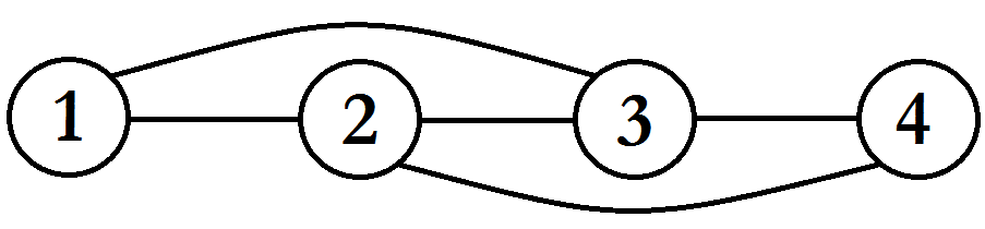
where is the equilibrium point of the oscillator, is a matrix consisting of the self frequencies, and is a damping matrix, which is positive-definite. The exact values of the matrices and -s were randomly chosen. The underlying graph is given in Figure 3.
The steady-state input-output relation if can be computed to be , whose inverse is . This gives us the convex function , which is strictly convex.
We wish to solve the synthesis problem for , where the controllers are taken to be identical and equal to
The function is given as
where is the sign function. One can verify that and that is a monotone ascending function. The associated integral function is given by:
We then use the formation reconfiguration scheme to create an augmented controller, where we use the first node as a leading node. The control objective was changed every 30 seconds according to the following desired steady-states,
where the first two entries refer to the first agent, the next two refer to the second agent, and so on. The output of the system can be seen in Figure 4, exhibiting the positions of the agents . The blue line represents first coordinate, and the red one represents the second coordinate. We can see that the agents act as expected, converging to the desired formations.
VI Conclusion
We have found a profound connection between passivity-based cooperative control and network optimization theory in the spirit of Rockafellar [17]. This was done by introducing the notion of maximal equilibrium-independent cyclically monotone passive systems, and showing that such systems converge to a solution of a collection of network optimization problems, bonded by duality. Furthermore, we have shown that in the case of output-agreement problems, the output agreement steady-state is optimal with respect to the optimal flow and optimal potential problems. This connection creates a dictionary between system signals (like outputs and inputs) and network optimization variables (potentials and node divergences, respectively). We have established analogous inverse optimality and duality results for general networks of maximal equilibrium-independent cyclically monotone passive systems. Using methods from subgradient theory and convex optimization, we have established clear criteria for solvability of the synthesis problem for a diffusive coupling of maximal equilibrium-independent cyclically monotone passive systems, and a practically-justifiable plant augmentation procedure to solve the synthesis problem if it is not feasible for the desired output. We have shown a synthesis for the controllers, and exhibited a controller augmentation procedure that allows any set of maximally equilibrium-independent cyclically monotone passive controllers to be used. This theory was exemplified by simulating a system of damped planar oscillators and correctly predicted the asymptotic state of the system, using both the minor controller and plant augmentation procedures. We believe that this strong connection between passivity-based cooperative control and network optimization theory can lead to new analysis methods for cooperative control problems, through the means of network optimization problems.
This is a significant extension of the framework connecting multi-agent systems and cooperative control to network optimization, first presented in [14] and later developed in [15]. Possible further research directions can include extensions of the framework (e.g., to directed graphs, passivity-short systems, and systems with different input and output dimension), or applications of the framework to yield various results in multi-agent systems (e.g. fault detection and isolation, network identification, robustness, etc.).
References
- [1] P. Iñigo-Blasco, F. D. del Rio, M. C. Romero-Ternero, D. Cagigas-Muñiz, and S. Vicente-Diaz, “Robotics software frameworks for multi-agent robotic systems development,” Robotics and Autonomous Systems, vol. 60, no. 6, pp. 803 – 821, 2012.
- [2] A. Quteishat, C. P. Lim, J. Tweedale, and L. C. Jain, “A neural network-based multi-agent classifier system,” Neurocomputing, vol. 72, no. 7, pp. 1639 – 1647, 2009. Advances in Machine Learning and Computational Intelligence.
- [3] S. Trip, M. Bürger, and C. D. Persis, “An internal model approach to (optimal) frequency regulation in power grids with time-varying voltages,” Automatica, vol. 64, pp. 240 – 253, 2016.
- [4] M. Mesbahi and M. Egerstedt, Graph Theoretic Methods in Multiagent Networks. Princeton Series in Applied Mathematics, Princeton University Press, 2010.
- [5] M. Arcak, C. Meissen, and A. Packard, Networks of Dissipative Systems. Springer International Publishing, 2016.
- [6] M. Arcak, “Passivity as a design tool for group coordination,” IEEE Transactions on Automatic Control, vol. 52, pp. 1380–1390, Aug. 2007.
- [7] N. Chopra and M. W. Spong, Advances in Robot Control: From Everyday Physics to Human-Like Movements, ch. Passivity-Based Control of Multi-Agent Systems, pp. 107–134. Springer, 2006.
- [8] L. Scardovi, M. Arcak, and E. Sontag, “Synchronization of interconnected systems with applications to biochemical networks: An input-output approach,” IEEE Transactions on Automatic Control, vol. 55, pp. 1367–1379, June 2010.
- [9] G.-B. Stan and R. Sepulchre, “Analysis of interconnected oscillators by dissipativity theory,” IEEE Transactions on Automatic Control, vol. 52, pp. 256–270, Feb. 2007.
- [10] A. J. van der Schaft and B. M. Maschke, “Port-hamiltonian systems on graphs,” SIAM Journal on Control and Optimization, vol. 51, no. 2, pp. 906–937, 2013.
- [11] Y. Tang, Y. Hong, and P. Yi, “Distributed optimization design based on passivity technique,” in 2016 12th IEEE International Conference on Control and Automation (ICCA), pp. 732–737, June 2016.
- [12] G. H. Hines, M. Arcak, and A. K. Packarda, “Equilibrium-independent passivity: A new definition and numerical certification,” Automatica, vol. 47, no. 9, pp. 1949––1956, 2011.
- [13] J. W. Simpson-Porco, “Equilibrium-Independent Dissipativity with Quadratic Supply Rates,” ArXiv e-prints, Sept. 2017.
- [14] M. Bürger, D. Zelazo, and F. Allgöwer, “Duality and network theory in passivity-based cooperative control,” Automatic, vol. 50, no. 8, pp. 2051––2061, 2014.
- [15] M. Sharf and D. Zelazo, “A network optimization approach to cooperative control synthesis,” IEEE Control Systems Letters, vol. 1, pp. 86–91, July 2017.
- [16] A. Jain, M. Sharf, and D. Zelazo, “Regularization and feedback passivation in cooperative control of passivity-short systems : A network optimization perspective,” IEEE Control Systems Letters, vol. 2, pp. 731–736, July 2018.
- [17] R. T. Rockafellar, “Characterization of the subdifferentials of convex functions,” Pacific Journal of Mathematics, vol. 17, no. 3, pp. 497––510, 1966.
- [18] S. Boyd and L. Vandenberghe, Convex Optimization. Cambridge University Press, 2004.
- [19] A. Pavlov and L. Marconi, “Incremental passivity and output regulation,” in Proceedings of the 45th IEEE Conference on Decision and Control, pp. 5263–5268, Dec 2006.
- [20] R. T. Rockafellar, Convex Analysis. Princeton Landmarks in Mathematics and Physics, Princeton University Press, 1997.
- [21] T. H. Cormen, C. E. Leiserson, R. L. Rivest, and C. Stein, Introduction to Algorithms, Third Edition. The MIT Press, 3rd ed., 2009.
- [22] C. Godsil and G. Royle, Algebraic Graph Theory. Graduate Texts in Mathematics, Springer New York, 2001.
- [23] M. Sharf and D. Zelazo, “On certain properties of convex funcions.” Available on arXiv:1703.00867 [math.OC].
- [24] A. J. van der Schaft and D. Jeltsema, Port-Hamiltonian Systems Theory: An Introductory Overview. Now Publishers Inc, 2014.
- [25] M. K. Camlibel and A. J. van der Schaft, “Incrementally port-hamiltonian systems,” in 52nd IEEE Conference on Decision and Control, pp. 2538––2543, 2013.
- [26] C. Zhao, U. Topcu, N. Li, and S. Low, “Design and stability of load-side primary frequency control in power systems,” IEEE Transactions on Automatic Control, vol. 59, no. 5, pp. 1177–1189, 2014.
- [27] T. Ishizaki, A. Ueda, and J. i. Imura, “Convex gradient controller design for incrementally passive systems with quadratic storage functions,” in 2016 IEEE 55th Conference on Decision and Control (CDC), pp. 1721–1726, Dec 2016.
- [28] A. Hatcher, Algebraic Topology. Cambridge University Press, 1st ed., 2001. p. 114–115.
This appendix deals with the proof of Theorem 8. The proof is rather lengthy, and requires two lemmas The idea is to try and construct a quadratic Lyapunov function of the form , where the point is a fixed point of the flow. Thus, we need to find a point which satisfies . The following two lemmas will assure that such a point exists.
Lemma 1.
Let be a strictly convex function, and suppose that as . Then there exists some , such that for every point satisfying , the inequality holds.
Proof.
Fix some arbitrary unit vector , and consider the convex function and its derivative . Note that because grows faster than any linear function, the same can be said about , and in particular, it’s derivative tends to infinity. Furthermore, the function is strictly convex, so is strictly ascending, Thus there is some such that if and if .
Our task now is to show that is a bounded function of . Suppose not, and let be a sequence of unit vectors such that . Passing to a subsequence, we may assume without loss of generality that for some unit vector . There is some such that if then . In particular, for but . This is impossible, as the first expression is equal to , which converges to the second expression, which is . Thus, there is some such that for all unit vectors , meaning that if is a vector of norm , then for :
| (25) |
∎
Lemma 2.
Let be a continuous vector field, and let . Suppose that for any vector satisfying , the inequality holds. Then there exists some point satisfying such that .
In order to prove the lemma, we use a theorem from algebraic topology.
Theorem 11 (Brouwer’s Fixed Point Theorem [28]).
Let be a closed ball inside , and let be a continuous map. Then has a fixed point.
Now, we prove the lemma.
Proof.
Suppose, heading toward contradiction, that does not vanish at any point in the ball . We define a map by
| (26) |
This is a continuous map (as never vanishes), and the norm of is always equal to , so is indeed in . Thus, we can apply Brouwer’s fixed point theorem to and get a fixed point, called .
We know that satisfies , i.e., . On one hand, taking the norm of the last equation implies that . On the other hand, rearranging it implies that where is some negative scalar (as ). Thus, we found a point of norm such that for some , which contradicts our assumption. Thus has a zero inside the ball . ∎
We are now ready to prove Theorem 8.
Proof.
First, because is constant, we can absorb the constant term inside the gradient by adding the linear term to . This does not change the fact that is strictly convex, nor the fact that it ascends faster than any linear function. Thus we may assume that for the remainder of the proof.
Now, we define the vector field . Note that because is skew-symmetric, for all ,
| (27) |
Thus, by the Lemma 1, there’s some such that for any vector satisfying , and by Lemma 2 we can find some point such that , or equivalently, . We claim that any solution to the ODE converges to .
Indeed, define . Then is non-negative, and vanishes only at , and furthermore,
| (28) |
where the last inequality is true because is convex and Theorem 2. Furthermore, is negative if because is strictly convex and Theorem 2. The uniqueness of follows from the fact that the flow globally asymptotically converges to . This completes the proof. ∎