Harmonic density interpolation methods for high-order evaluation of
Laplace layer potentials in 2D and 3D
Abstract
We present an effective harmonic density interpolation method for the numerical evaluation of singular and nearly singular Laplace boundary integral operators and layer potentials in two and three spatial dimensions. The method relies on the use of Green’s third identity and local Taylor-like interpolations of density functions in terms of harmonic polynomials. The proposed technique effectively regularizes the singularities present in boundary integral operators and layer potentials, and recasts the latter in terms of integrands that are bounded or even more regular, depending on the order of the density interpolation. The resulting boundary integrals can then be easily, accurately, and inexpensively evaluated by means of standard quadrature rules. A variety of numerical examples demonstrate the effectiveness of the technique when used in conjunction with the classical trapezoidal rule (to integrate over smooth curves) in two-dimensions, and with a Chebyshev-type quadrature rule (to integrate over surfaces given as unions of non-overlapping quadrilateral patches) in three-dimensions.
Keywords: Laplace equation, layer potentials, boundary integral operators, Taylor interpolation, harmonic polynomials, Nyström method
AMS subject classifications: 65N38, 35J05, 65T40, 65F08.
1 Introduction
The numerical solution of linear constant coefficient partial differential equations (PDEs) by boundary integral equation (BIE) methods provide several advantages over methods based on volumetric discretizations such as finite difference and finite element methods. Indeed, BIE methods can easily handle unbounded domains as they are based on the discretization of the relevant physical boundaries, giving rise to well-conditioned linear systems of reduced dimensionality. Although dense, these linear systems can be efficiently solved by means of iterative solvers in conjunction with fast methods such as the Fast Multipole Method [22], -matrix compression [23], or FFTs based on equivalent-sources methods [15, 43].
One of the main attractive features of BIE discretizations is their ability to deliver high-order convergence. The latter is typically achieved by specialized quadratures carefully designed for the resolution of the singular behavior of the kernels of the operators that enter the BIE. As is known BIE rely on layer potentials defined in terms of the Green function of the underlying PDE and its derivatives. The boundary values of these layer potentials, in turn, give rise to certain boundary integral operators (BIOs) which enter the BIE. For instance, in the case of the Laplace equation under consideration, the boundary values of the single- and double-layer potentials and their normal derivatives give rise to four BIOs; single-layer, double-layer, adjoint double-layer, and hyper-singular operators. These four BIOs constitute the building blocks of all possible BIE formulations of Laplace equation. The kernels of the four Laplace BIOs feature the Green function of the Laplace equation and its various normal derivatives, and thus they exhibit different singular behaviors. Indeed, in the case of regular boundaries, (1) the single-layer operators feature weakly singular (integrable) kernels in both two and three dimensions, (2) the double-layer operators feature regular kernels in two dimensions, and weakly singular kernels in three dimensions, and (3) the hyper-singular operators in both two and three dimensions feature boundary integrals that have to be understood in the sense of Hadamard finite-parts integrals. In addition, the evaluation of layer potentials near (but not on) boundaries is faced with the significant challenge of resolving nearly singular kernels.
1.1 Previous work
Significant efforts have been directed toward the development of high-order quadrature rules for the numerical evaluation of singular and nearly singular boundary integral operators over the last decades. Most of these quadratures are geared toward two dimensional applications and rely on analytical resolution of singularities. As such, the quadratures become more involved as the kernels become more singular. A comprehensive methodology for high-order evaluations of BIOs on smooth (two-dimensional) curves, which relies on global trigonometric interpolation, logarithmic kernel singularity splitting and resolution of logarithmic singularities, was put forth by Martensen [39] and Kussmaul [36]11 1 A concise presentation of the Martensen-Kussmaul quadrature rule can be found in [19, Chapter 2]. This method was subsequently extended by Kress to deliver high-order Nyström discretizations of boundary integral equations posed on curves with corners [33] and to boundary integral equations involving singular kernels that arise from a regularization of the hypersingular operator [34]. Other high-order, yet not spectrally accurate, methods—some of which are applicable to a more general class curves in the plane—have been presented in numerous contributions [3, 28, 25, 32, 41]. However, the treatment of nearly singular operators in the context of the methods mentioned above requires post-processing steps such as oversampling of densities and interpolation/extrapolation procedures.
Motivated in part by fluids applications involving simulation of Stokes flow in multiply connected domains, recent efforts targeted the development of high-order quadratures that can evaluate seamlessly both singular and nearly singular Laplace kernel interactions. Notably, Quadrature by Expansion (QBX) methods have successfully bypassed the need to directly deal with singular integrands [31] by relying on kernel-specific expansions (based on addition theorems for Green’s functions) of the layer potentials around points (centers) near the boundary. It is also worth mentioning the second-order accurate scheme of Beale et al. [8] for evaluation of nearly singular integrals in 2D, which is based on a certain mollification and asymptotic correction of the integral kernel. Substantially more accurate and sophisticated numerical procedures to deal with nearly singular integrals were developed by Helsing et al. [26] (which was later improved in [5]) and by Barnett [6], the latter of which provided the basis for QBX methods [31]. However, besides the fact that some of the more recent proposed approaches for singular and nearly singular integrals do not easily generalize to three-dimensions (3D), we believe it is fair to claim that, given their level of sophistication, these methods are arguably difficult to implement. Indeed, the high accuracy achieved by these methods is a result of a judicious combination of involved techniques encompassing grid oversampling of the density, kernel approximations and/or expansions, and high-order polynomial interpolation. In addition, and perhaps more importantly, all the aforementioned methods require a careful selection of several parameters in order to garner their optimal performance. The selection of the parameters needed in 2D QBX (e.g. location of off-surface centers, order of expansions in the kernel representation, oversampling factors), for instance, can be streamlined by resorting to local kernel expansions in a version of QBX referred to Adaptive Quadrature by Expansion (AQBX) [30].
There are significantly fewer high-order methods for the discretization 3D Laplace BIEs with respect to their 2D counterparts. This fact can be explained by the additional challenges that pertain to 3D, amongst which we mention (a) the more severe nature of the singularities of the Green functions and their derivatives, (b) the technical difficulties associated with the reliable generation of high-order surface representations, and (c) the need to employ patches in order to describe surfaces as well as local approximations of densities. First, we remark that the singularities of BIOs—in particular that of the hyper-singular one—are more challenging for Nyström discretizations than for Galerkin (BEM) discretizations, as weak formulations of Laplace BIEs require (double) integration of weak singularities only. We also note that with regards to the latter aspect (c), the use of non-overlapping patches (which is the most natural in our opinion) inherently gives rise to nearly singular integrands corresponding to the scenario when the target and integration points are nearby yet they belong to adjacent but different patches. The resolution of near singularities, encountered mostly in Galerkin discretizations, can be effected by double exponential (e.g., , ) changes of variables [51] or using the singular quadratures of Sauter and Schwab [45]. Singularity subtraction techniques are certainly the most common approach for evaluating singular integrals arising from BIEs and, therefore, numerous low-order variants of these techniques are available in the literature not only for the Laplace equation but also for the Helmholtz, Stokes flow and elastostatic equations. A notable exception is the high-order version of the singularity subtraction approach proposed in [24] for Nyström discretizations of BIOs on tori. Regardless of discretization type, most 3D high-order quadratures of BIOs are case specific, that is, they are designed to specifically treat a certain type of kernel singularity or near-singularity, and become increasingly involved as the kernel singularity becomes more severe. Owing to these difficulties, the implementation of high-order numerical methods for evaluation 3D Laplace BIEs is complex, arguably leading to a dearth of available open-source software (BEMpp [48], https://bempp.com, being a notable exception) and ultimately limiting wider use in the engineering community. Without being exhaustive, in what follows we review several high-order Nyström numerical schemes for solution of 3D Laplace BIEs.
A spectrally accurate Nyström method for 3D BIEs in the spirit of Martensen and Kussmaul was developed by Ganesh et al. [21] for surfaces diffeomorphic with spheres. This approach makes use of the diffeomorphism between the surface of integration and the unit sphere, global interpolation of densities in terms of spherical harmonics, as well as addition theorems that lead to analytic resolution of weak kernel singularities. Stronger kernel singularities can be handled via integration by parts techniques. We mention that variants of this approach have been used in Stokes flow simulations [55]. A more general high-order Nyström method for the solution of BIEs on smooth surfaces is the (provably convergent) method of Bruno at al. [11, 15, 16]. The essential ingredients of this method consist of (1) use of an explicit atlas of overlapping patches and associated partition of unity functions and (2) use of polar change of variables to analytically resolve weak kernel singularities. The method is quite general, as it was demonstrated in [14, 58] that surfaces of engineering relevance can be accurately approximated by means of smooth overlapping-patch manifold representations. The change to polar coordinates approach was extended and refined in [10] via additional affine mappings and precomputed quadrature tables, to treat cases when the surface parametrizations are highly non-conformal. This approach was extended to deal with singular integral operators in subsequent contributions [12, 17, 57]. In turn, several post processing techniques have been proposed in the literature to deal with nearly singular-integrals in 3D. We mention first the “extraction” technique of Schwab et al. [46] which, using Taylor expansions along the unit normal to the surface, allows for approximations of layer potentials near and on the surface. The higher-order terms in the Taylor expansions, however, involve high-order normal derivatives which incur the significant overhead of evaluating several strongly singular boundary integral operators. Yet another procedure to deal with nearly singular integrands in 3D was presented in [57]. Unlike [46], this procedure makes used of both on- and off-surface values (at points sufficiently far away from the surface with respect to the mesh size) to interpolate layer potentials near the boundary. A simple method based on a kernel regularization that can achieve high-order evaluations of both singular and nearly singular Laplace boundary integrals was put forth by Beale in [7] and then further developed in [9] and even extended to Stokes flow equations in [52]. This kernel regularization delivers third-order methods for on-surface as well as near-surface evaluations of the single and double-layer Laplace BIOs. One of the main advantages of Beale’s kernel regularization method is that it does not require a surface parametrization nor a surface triangulations. Finally, we mention the very recently introduced extensions of QBX methods to evaluations of 3D boundary integral operators/ layer potentials [1, 47]. Just like the kernel regularization methods [9], QBX methods can seamlessly treat both weakly singular and nearly singular boundary integral operators/layer potentials in 3D; however, evaluations of adjoint double-layer and hyper-singular boundary integral operators or their Stokes counterparts with commensurate orders of singularity are not presented in [1, 47].
1.2 Scope of this contribution
This paper presents a novel harmonic density interpolation method that regularizes the kernel singularities of the four BIOs associated with the Laplace equation in smooth two- and three-dimensional domains. Unlike singularity subtraction techniques, our method achieves regularization of the integral kernels by targeting the densities of the BIOs instead of the kernels themselves. Low-order precursors of regularization techniques that target the integral densities are available in the literature for BIOs associated with various linear constant coefficient PDEs [29, 37, 38, 42, 49]. In certain aspects the proposed method is a generalization of the third-order regularization technique introduced in [42] for the 2D Helmholtz combined field integral operators. The main contribution of this paper consists of developing a high-order local Taylor-like interpolation methodology based on harmonic polynomials that takes full advantage of the boundary regularity of the density functions that enter Laplace BIOs. Our approach is universal, in the sense that is applicable to evaluations of all four Laplace BIOs irrespective of the singularity of their associated kernels. In detail, in order to evaluate the single-layer operator in , ,
for example, where is the free-space Laplace Green function and is a regular density function defined on a closed boundary , we make use of a family of smooth harmonic functions and Green’s third identities to recast in the form
We require then to be such that both expressions and , where denotes the normal derivative with respect to , vanish to prescribed orders as . The key insight of our method is to seek families of functions of the form
where are homogeneous harmonic polynomials of order . Thus, the requirement that the expressions and vanish simultaneously to high-order as is equivalent to solving for each point a local Taylor-like interpolation problem of prescribed order involving the density function and Dirichlet and Neumann boundary values of harmonic polynomials in the above definition of the functions . In 2D, such families of functions can be easily obtained to arbitrarily high-order by means of complex variable techniques. In 3D, in turn, their construction is significantly more involved, yet it is relatively easy to produce third-order interpolating functions . The proposed technique extends naturally to deal with nearly singular integrands, allowing layer potentials and their gradients to be evaluated at target points arbitrarily close to the boundaries without compromising numerical accuracy. The high-order harmonic density interpolation method renders the Laplace BIOs directly amenable to evaluations by standard, readily implementable quadrature rules (e.g. trapezoidal rule in 2D, and Fejér, Clenshaw-Curtis quadrature in 3D) as the BIOs feature only regular (at least continuous for weakly singular BIOs and bounded for the hypersingular BIO in 3D) integrands. The integration of our method within the FMM framework is fairly straightforward and will be presented in a future contribution.
We illustrate the effectiveness and simplicity of the proposed high-order harmonic density interpolation technique through a variety of 2D and 3D numerical results concerning evaluation of singular and nearly singular Laplace BIOs and layer potentials defined on closed, smooth curves and surfaces. We show, in particular, that for sufficiently high interpolation orders (which achieve integrands that vanish as at the kernel singularity ) our technique used in conjunction with the simple trapezoidal quadrature leads to discretization errors in the evaluation of the two-dimensional single-layer BIO of the order for even, and respectively for odd, where denotes the grid spacing. In addition, the same methodology leads to evaluations of the 2D hyper-singular BIO that converge exponentially fast. For 3D problems, in turn, we provide the explicit construction of the harmonic polynomial interpolants amenable to express the single- and double-layer operators in terms of continuous integrands, and the adjoint double-layer and hypersingular operators in terms of bounded integrands. Relying on a non-overlapping quadrilateral patch manifold representation of 3D surfaces, underlying local Chebyshev grids, and a (spectrally accurate) Fejér quadrature rule [13, 54], we demonstrate through numerical examples that the proposed harmonic density interpolation technique yields a third-order accurate Nyström method for BIEs involving the Laplace single- and double-layer operators, and a second-order accurate Nyström method BIEs involving the Laplace adjoint-double layer and hypersingular operators. The levels of accuracy achieved by our method for three dimensional problems (e.g., ) are competitive for engineering applications, especially in the light of the straightforward implementation of the method. A preliminary Matlab implementation of the proposed methodology for 3D problems is available at:
https://github.com/caperezar/HDIMethod.
We also mention that the proposed harmonic density interpolation can easily accommodate evaluations of nearly singular boundary integral operators. Extensions of our method to treatment of singular and nearly singular BIOs arising in acoustics, electromagnetics, and elastodynamics are currently being pursued; for those problems the local Taylor-like interpolation problems will rely on plane-waves rather than harmonic polynomials.
The structure of this paper is as follows. Sections 2, 3 and 4 provide a comprehensive description of the proposed technique for 2D BIEs. The details on the construction of the harmonic expansion functions using complex variable techniques are given in Section 3. Section 4 presents the extension of the technique for the evaluation of layer potentials at target points near the boundary. The proposed technique for corresponding 3D problems is described in Section 5. Section 6, finally, presents a variety of numerical examples in two and three spatial dimensions, including comparisons with Beale et al. [8, 59] and QBX [31] methods in 2D.
2 High-order kernel singularity regularization for 2D problems
The single-layer (), double-layer (), adjoint double-layer () and hypersingular () operators of Calderón calculus associated with the Laplace equation in are given by
| (1a) | ||||
| (1b) | ||||
| (1c) | ||||
| (1d) | ||||
for , where
| (2) |
is the free-space Green function for the Laplace equation in , and f.p. in equation 1d stands for the Hadamard finite-part integral. The curve in 2D is assumed to be a simple closed curve that admits a regular periodic counterclockwise parametrization
| (3) |
In the parameter space the four integral operators defined in equation 1 will be denoted by , , and , where . For presentation simplicity throughout this paper both the density function and the curve parametrization are assumed to be analytic functions of . Note that under the assumptions introduced above, and in the particular case of the Laplace equation in two spatial dimensions, the integral kernels in both double-layer () and adjoint double-layer () operators are smooth functions (see Lemmas 2.1 and 2.2), so their high-order numerical evaluation can be achieved by application of standard quadrature rules (e.g. trapezoidal rule). A more general analysis can be carried out to significantly relax the strong analytic regularity assumptions made on and (see Remark 2.3 below).
2.1 Hypersingular operator
Consider first the hypersingular operator , defined in equation 1d, applied to a smooth density function , and evaluated at a point . The proposed technique relies on introducing a known smooth function , with Dirichlet and Neumann traces denoted by and for , respectively, such that
| (4) |
can be evaluated by integrating regular (non-singular) functions only. Given the strong singularity of the hypersingular operator kernel, it is thus necessary that vanishes to high order as . Additionally, we need to admit a representation in terms of smooth integrands as well. The key idea of our method is to choose to be harmonic in the first variable, so that by Green’s third identity [40] we have
| (5) |
Therefore, we can then express the hypersingular operator as
| (6) |
where the integrals on the right-hand-side involve functions with smoothness that can be controlled by an appropriate choice of , i.e., by requiring to vanish to high enough order as . In detail, for a prescribed density interpolation order , we require to satisfy the following condition
| (7) |
We also require that the constants in the “big-” notation in equation (7) be bounded uniformly in . Relying on the smoothness of both and it easy to show (using Taylor’s theorem) that a sufficient condition for equation 7 to hold is that satisfies
| (8) |
or equivalently, that the -th Taylor expansion coefficient of equals the -th order derivatives of at . Note that on account of the smoothness of the kernel of the operator , we do not impose any vanishing conditions on the expressions as . Remarkably, and as we will explain in the next sections, our construction of the harmonic functions that meet the requirement (8) achieves as a byproduct a vanishing condition of order on .
The following lemma shows that choosing in the conditions equation 8 for , the hypersingular operator can be expressed in terms of integrals of (smooth) -periodic analytic functions.
Lemma 2.1.
Let be a closed simple analytic curve and be a real -periodic analytic function. Suppose there exists , harmonic in for all , such that its Dirichlet trace satisfies equation 8 for . Then, letting denote the Neumann trace of , the hypersingular operator can be expressed as
| (9) |
where
| (10) |
and
| (11) |
are real analytic -periodic functions of for all .
Proof.
The explicit expressions for in equation 10 and in equation 11 when are obtained from identity equation 6. Their values at , in turn, follow from a direct application of L’Hospital rule.
In order to prove the analyticity of and for , we first note that since the curve parametrization is analytic and -periodic, the following expressions hold: , and , where , and are analytic -periodic functions. Furthermore, since the curve parametrization is regular we have . By the interpolation conditions equation 8 and the fact that and are analytic -periodic functions (due to the fact that is the trace on of the harmonic function , which is analytic in all of ), on the other hand, it follows that with being an analytic -periodic function. Therefore, since by hypothesis of the lemma, we conclude that equation 10 and equation 11 are analytic -periodic functions of with a removable singularity at . The proof is now complete. ∎
2.2 Single-layer operator
A calculation similar to the one shown above for the hypersingular operator yields that can be expressed as
| (12) |
for . Hence, in order for the right-hand-side of equation 12 to be given in terms of integrals of smooth functions, we need to find a harmonic function with Neumann trace satisfying
| (13) |
Again, we do not formally impose any vanishing conditions on the expressions as , yet our construction of the harmonic functions will automatically realize such conditions of order . The following lemma shows that the single-layer operator can in fact be expressed in terms of smooth integrands provided the interpolation conditions equation 13 are satisfied.
Lemma 2.2.
Let be a closed simple analytic curve and be a real -periodic analytic function. Suppose there exists , harmonic in for all , such that its Neumann trace satisfies equation 13 for . Then, letting denote the Dirichlet trace of , the single-layer operator can be expressed as
| (14) |
where
| (15) |
is a analytic -periodic function of , and
| (16) |
is a -times continuously differentiable -periodic function of , for all . Furthermore, the -th derivative of is an integrable function for all
Proof.
The explicit expressions for the integrands in equation 15 and equation 16 are obtained directly from identity equation 12. The proof that is an analytic -periodic function, on the other hand, is essentially the same as in the case of in Lemma 2.1, so it is omitted here.
Since both and are analytic -periodic functions we have that can be expressed as with being analytic and -periodic. Therefore, adding and subtracting the function to in equation 16 we obtain with being analytic and -periodic. Therefore, by the product rule we readily obtain that the -th order derivative of is a -periodic function that vanishes as as , so it is indeed continuous at . The -th order derivative of , in turn, features a integrable singularity as . The proof is now complete. ∎
Remark 2.3.
The analytic regularity of both the curve and the density function assumed in this section can be significantly relaxed. Indeed, straightforward modifications of Lemmas 2.1 and 2.2 can be carried out to show that for of class and of class , with and , the proposed density interpolation technique yields -periodic -times continuously differentiable integrands in the cases of the hypersingular, double-layer, and adjoint double-layer operators, and it yields -periodic -times continuously differentiable integrands in the case of the single-layer operator.
It is also worth mentioning that the proposed technique can in principle be extended to piecewise smooth curves in 2D when the (global) parametrization of the curve and the layer potential densities are not differentiable at corners. The lack of smoothness at corners can be circumvented in practice by discretizing the smooth panels using grids that (i) are refined toward corner points and (ii) do not include corner points (e.g. Chebyshev nodes). As demonstrated in the numerical experiments in Section 6.4 below, this approach works well in 3D for low-order interpolations order (see also [42] for a related approach for the 2D Helmholtz equation using graded meshes constructed via sigmoid transforms).
In the next section we provide a procedure to construct harmonic interpolating functions and satisfying the conditions in Lemmas 2.1 and 2.2, respectively, for any given density interpolation order .
3 Harmonic interpolating functions in 2D
In order to construct the desired harmonic functions in Lemmas 2.1 and 2.2, we consider linear combinations of harmonic polynomials of the form
| (17) |
where , with , and , for . Instead of working with the real expression (17) it turns out to be convenient to complexify it and consider instead where
| (18) |
with denoting the curve in the complex plane parametrized by the (analytic) complex valued function , We here recall that the curve is parametrized by , . Clearly, (by the Cauchy-Riemann equations) is harmonic in .
Letting then , , and calling for in (18), we obtain the expressions
| (19a) | ||||
| (19b) | ||||
for the Dirichlet and Neumann traces of (in the parameter space), respectively, where we made use of the identity . Furthermore, it is easy to show that
| (20a) | ||||
| (20b) | ||||
for , where by the Faà di Bruno formula we have
| (21) |
with and , , denoting the so-called partial or incomplete Bell polynomials; cf. [2, Chapter 13].
In what follows of this section we use the identities (20) and (21) to show that given a density interpolation order , there exist harmonic functions and satisfying the interpolating conditions in equation 8 and equation 13, where and are functions of the form equation 18.
3.1 Interpolating function for the hypersingular operator
We start by seeking coefficients in the expansion
| (22) |
so that the interpolation conditions equation 8 are satisfied. In view of equations equation 20, we then note that conditions equation 8 can be enforced on by requiring to satisfy
| (23) |
Clearly, the condition in equation 23 implies that . Taking then in equation 22 we get from equation 21 that the remaining conditions (for ) can be expressed as the linear system
| (24) |
whose unknowns are the coefficients , where the entries of the matrix function are given by
| (25) |
and where the vector on the right-hand-side of equation (24) is given explicitly by . The matrix defined in equation 25 is sometimes referred to as Bell matrix; cf. [2, Chapter 13].
Since is a lower triangular matrix and its diagonal terms are [2, Chapter 13], where for all (i.e., the curve is regular), we readily conclude that the linear system equation 24 is invertible for all . Therefore, having retrieved the coefficients from solving the linear system equation 24, we immediately obtain and .
Given that the matrix is lower triangular, the solution of the linear system equation 24 can be obtained using forward substitution. For the density interpolation order , for example, the matrix is explicitly given by
Matrices corresponding to orders are simply submatrices of the matrix displayed in section 3.1.
Remark 3.1.
It follows from equation 23, and the fact that is real-valued, that
Therefore, , defined as in equation 19b in terms of , satisfies
and, consequently, as . This fact will play an important role in section 4, where an extension of the proposed density interpolation technique is presented for the regularization of nearly singular integrals.
3.2 Interpolating function for the single-layer operator
A procedure similar to the one described above for the construction of allows us to find the coefficients in the expansion
| (31) |
In fact, in view of identities equation 20, conditions equation 13 can be enforced on by requiring to satisfy
| (32) |
Conditions equation 32 do not pose any constrain on , so we may set . Letting then in equation 31 we obtain that conditions equation 32 are fulfilled if and only if satisfies
| (33) |
where is the lower-triangular matrix
| (34) |
is the Bell matrix equation 25, and . Since both and are invertible matrices (none of the diagonal entries of is zero), the coefficients in the expansion equation 31 are uniquely determined by the linear system equation 33. Having found the coefficients , we obtain and .
Remark 3.2.
Note that equation 32, the choice , and the fact that is real-valued, imply that that satisfies
for . Therefore as . This identity, together with Remark 3.1, will be used in section 4 to extend the proposed density interpolation technique to the regularization of nearly singular integrals.
Remark 3.3.
If an arc-length parametrization of the curve is considered, i.e., where is the length of the curve and for all , then the matrix in equation 33 becomes the identity matrix and the linear systems equation 48 and equation 33 differ only by the right hand side. Although in theory it is always possible to re-parametrize a smooth regular curve by its arc-length, there are practical advantages of considering the more general parametrization equation 3 assumed here.
As announced, in the next section we present and extension of the harmonic interpolation technique to the regularization of nearly singular integrals.
4 Nearly singular integrals in 2D
The single- and double-layer potentials are respectively defined as
| (35) |
for , which, using the curve parametrization in 2D, become
| (36a) | ||||
| (36b) | ||||
where . As it is well known, the kernels in equation 36 become nearly singular (i.e., develop sharp peaks) as the target point approaches the boundary , making the numerical evaluation of equation 36 challenging. In this section we show that the harmonic interpolating functions and constructed in section 3 can be effectively used to effectively regularize the kernels of both layer potentials.
We first note that by Green’s third identity, any function harmonic in the first variable, satisfies
| (37) |
where if lies inside the domain enclosed by , and otherwise. Using this identity and recalling that and denote the Dirichlet and Neumann boundary values of on , we have that the single-layer potential can be expressed as
| (38) |
while the double-layer potential can be expressed as
| (39) |
for all and .
In order to smooth out the nearly singular integrands in equation 38 and equation 39 that arise for points close to , we let in equation 38 and in equation 39, where and are the harmonic interpolating functions constructed in section 3. The expansion point is then selected as with , where we assume that is sufficiently close to so that this minimizer is unique. Doing so, and in view of the fact that and as (see Remark 3.2), we obtain that the integrands in equation 38 satisfy
| (40a) | ||||
| (40b) | ||||
as . Similarly, recalling that and as (see Remark 3.1), it can be shown the integrands in equation 39 satisfy
| (41a) | ||||
| (41b) | ||||
as , where is the prescribed harmonic interpolation order. The asymptotic identities equation 40 and equation 41 show that the smoothness of the integrands at and around the nearly singular point can be controlled by means of our technique.
As shown in [42, Section 3.4], the proposed technique can also be utilized to regularize the kernels that arise in problems involving multiply connected domains with boundary components that are close to each other. In this case, nearly singular integrals associated with any of the integral operators equation 1 can be directly computed by evaluating the regularized expressions for the layer potentials equation 38 and equation 39, or their respective normal derivatives on a curve that does not intersect . The numerical results presented in this paper demonstrate the effectiveness of the proposed technique for the regularization of nearly singular integrals.
5 High-order kernel singularity regularization for 3D problems
As it turns out, most of the ideas presented above in this paper for the Laplace boundary integral operators in 2D can be directly generalized to 3D. Indeed, letting denote harmonic functions (in the first variable) in all of it can be shown—using Green’s third identity—that for a smooth closed oriented surface the four integral operators of Calderón calculus can be expressed as
| (42a) | ||||
| (42b) | ||||
| (42c) | ||||
| (42d) | ||||
for , where the definition of the boundary integral operators , , and is the same as the one given in equation (1), except for the fundamental solution of the Laplace equation whose expression in 3D is
| (43) |
Note that unlike the 2D case, the kernels of the operators and are (weakly) singular, and thus all the four Laplace boundary integral operators in 3D require application of the density interpolation technique to achieve integral expressions in terms of more regular integrands.
In order to establish a set of point conditions on the Dirichlet and Neumann boundary values of and on that lead to more regular integrands in the expressions on the right-hand-side of (42), we resort to the local parametrization of the surface . It follows from the regularity of that at every point there exists a smooth local diffeomorphism , where is an open neighborhood of , in an open neighborhood of , and the mapping is such that . Resorting to the parametrization and the index notation for partial derivatives, i.e., letting , , and where denotes the derivative with respect to (), it can be shown that the point conditions
| (44a) | ||||
| (44b) | ||||
and
| (45a) | ||||
| (45b) | ||||
where and , suffice to guarantee that the estimates
hold true as , where all the constants in the “big-” notations above can be bounded uniformly in . Therefore, the smoothness of integrands in (42) is controlled by the regularization orders and , provided the requirements (44) and (45) are satisfied. We emphasize that unlike in the 2D case, there are more local vanishing conditions to be imposed in 3D per each point in order to achieve the same integrand regularization orders.
In the numerical examples considered in this paper we select and (i.e. the lowest values of these parameters that remove the singularity of the hyper-singular BIO and at the same time lead to integrands for the evaluation of both single and double-layer BIOs) and harmonic function functions and given in terms of linear combinations of homogeneous harmonic polynomials of order at most two. In detail we let
| (46) |
where the homogeneous harmonic polynomials utilized in the expansions above are
| (47) |
and the expansion coefficients and must be obtained by enforcing the point conditions (44) and (45) on and . In order to enforce such conditions, we first let and denote the Dirichlet and Neumann traces of the harmonic polynomials , respectively, where the unit normal at is given by Therefore, the enforcement of the points conditions (44) and (45), respectively, leads to the following linear systems
| (48) |
for the vectors of coefficients and , where the entries of the matrix are given by
| (49a) | ||||||||
| (49b) | ||||||||
| (49c) | ||||||||
for , and the right-hand-side vectors are
| (50) |
As discussed in Appendix A, the matrix is invertible for all the points on the surface and in fact, (we note here that represents the surface element, and thus the determinant of the 3D harmonic Taylor-like interpolation problem bears similarities to its 2D counterpart). Clearly, with the aforementioned selections the integrands on the right-hand-side of (42a) and (42b) become -functions, while the integrands in (42c) and (42d) become bounded functions. Higher-order versions of the harmonic interpolation technique (corresponding to larger values of the parameters and in equations (44) and (45)) can be pursued at the cost of incorporating higher-order harmonic polynomials in the Taylor-like interpolation scheme as well as higher-order derivatives of the surface parametrization and of the density . However, the invertibility of matrices corresponding to the ensuing interpolation problems (48) for higher values of the parameters and remains an open question (note that for the next density interpolation order, that is and , one would have to deal with matrices ). Nevertheless, the numerical results presented in Section 6.4 illustrate that the choice and already leads to very accurate results produced by a simple implementation.
As in 2D, nearly singular integrands arising due to observation points near the surface, can be regularized utilizing the harmonic functions and to interpolate the density function at the surface point . In particular, it follows from (35) and (37) that following expressions for the single- and double-layer potentials
| (51a) | ||||
| (51b) | ||||
hold for all , where if lies inside the domain enclosed by , and otherwise.
We present next a variety of numerical results that showcase the effectiveness of the regularization technique via harmonic density interpolation in both two and three dimensions.
6 Numerical examples and applications
6.1 Singular integrals in 2D
We first present a simple Nyström method based on the high-order harmonic density interpolation technique (referred to in what follows by the acronym HDI) for kernel regularization combined with the classical trapezoidal rule for the direct numerical evaluation of the single-layer and hypersingular operators. Given that we assumed throughout that the smooth closed curves are given in terms of smooth, periodic parametrizations, we consider a uniform discretization of the interval with grid points , for , where . Using global trigonometric polynomial interpolation of the densities , application of the trapezoidal rule leads to the following semi-discrete approximations of the parametrized single-layer and hyper-singular operators
| (52) | ||||
| (53) |
for , where , , and are defined in equation 10, equation 11, equation 15 and equation 16, respectively. The construction of all these functions is described in section 3 and requires computation of high-order derivatives of the parametrization as well as the trigonometric polynomial interpolants of at the grid points. Since the functions are -periodic and analytic, the derivatives of their trigonometric polynomial interpolants can be computed via FFT-based numerical differentiation with errors that decay exponentially fast as the size of the equi-spaced grid increases; cf. [50]. In light of Lemma 2.1, which established the smoothness and periodicity of and , we conclude that for any regularization order the trapezoidal rule approximation equation 52 of the hypersingular operator converges exponentially fast as increases [20, 53]. Finally, fully discrete approximations of the operators and are obtained by simply evaluating at the grid points their semi-discrete versions in equations (52) and respectively (53).
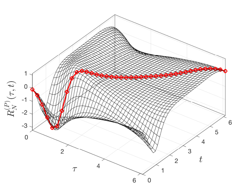
In order to demonstrate the fast convergence of the HDI approximation equation 52 of the hyper-singular operator, we present in Figure 1a maximum absolute errors on the circular boundary between our discretizations corresponding to harmonic interpolation orders and and a reference solution produced by the spectrally accurate evaluation of the hypersingular operator [35]. The reference solution was obtained using a refined uniform discretization of the interval with grid size . In the case of the application of the harmonic interpolation technique of order —the blue curve in Figure 1a, the (undefined) values of the integrand at were replaced by zero. As expected, for orders the kernel in equation 9 becomes analytic, and therefore exponential convergence of equation 52 is observed as increases. Figure 1b displays the smooth integrand resulting from application of the harmonic interpolation technique for .
For the single-layer operator, in turn, the order of convergence of the HDI discretization equation 53 is limited by the polylogarithmic singularity of (see Lemma 2.2). As increases, becomes smoother, but the logarithmic terms cannot be completely removed by the proposed technique. The effect of the smoothness of on the convergence of the HDI discretization is demonstrated in Figure 2, which displays the maximum absolute errors in the evaluation of the single-layer operators for even (Figure 3a) and odd (Figure 3b) regularization orders . The errors are measured with respect to a highly accurate evaluation of single-layer operator obtained by means of the Martensen-Kussmaul quadrature rule [36, 39] using a refined uniform grid with . Interestingly, as noted in Remark 6.1 below, an extra order of convergence is gained due to the symmetry of the integrand for even, which explains the fact that the same convergence rates are observed in Figures 3a and 3b for even and odd orders , respectively.
Remark 6.1.
It follows from [18]—where the Euler-Maclaurin formula in the presence of a logarithmic singularity is derived—that for an odd density interpolation order , , the approximation of the single-layer operator equation 53 yields errors of order .
For an even density interpolation order , , in turn, we can write where is an analytic -periodic function. Using this fact we have that in equation 14 can be expressed as
| (54) |
in terms of
and a -periodic analytic function that is integrated with exponentially small errors by the trapezoidal rule. Furthermore, we note that can be split as
| (55) |
Since the first term in equation 55 is a -periodic function that is odd with respect to any of the quadrature points , , it readily follows that the trapezoidal rule integrates it exactly (and yields 0). On the other hand, since the second term in equation 55 is a -periodic function of class and the first derivates of vanish at , we have from [18] again, that the trapezoidal rule applied to this term yields errors of order . From these observations we thus conclude that the trapezoidal rule approximation equation 53 yields errors of order for even .
Finally, in order to illustrate the competitiveness of the proposed HDI method we present comparisons with the recently introduced Quadrature-by-Expansion (QBX) method of Klockner et al. [31]. The reason why we consider the QBX method is that, just like the HDI kernel regularization method, the QBX method can deliver high-order discretizations of singular and nearly singular boundary integral operators in both two and three dimensions. For presentation simplicity we focus here on the evaluation of the single-layer operator. Following [4], we compute the single-layer operator by the surrogate expansion
| (56) |
where the expansion center lies at a distance away from the evaluation point along the normal direction to the curve, with (resp. ) corresponding to points lying outside (resp. inside) the curve. The coefficients in (56), in turn, are given by
| (57) |
and are computed by the trapezoidal rule on a uniform oversampled grid with points (). We use one expansion center per discretization point and the expansion center distance to the curve () is selected to be proportional to the local distance between the discretization points () in physical space. That is, the distance to the curve of the expansion center associated to the discretization point , , is proportional to
A straightforward comparison between QBX and the HDI method becomes somewhat difficult due to the selection of the various parameters involved. As shown by the analysis in [4, 31], the error in the QBX discretization is governed by a subtle balance between the order of the expansion (), the distance of the expansion centers from the curve (), and the oversampling ratio (). Figure 3 presents a comparison between the two methods where the errors in the evaluation of the single-layer operator are displayed for various choices of the QBX parameter, keeping the order and the oversampling ratio constant. To make the comparison fair, an oversampled grid with points is also utilized in the HDI single-layer evaluation. Although not necessarily optimal, the oversampling ratio and the harmonic interpolation order are used in both examples. We point out here, that since our technique requires the computation of high-order derivatives along the curve (that is the interpolation coefficients in equation (22) depend on derivatives of both the parametrization and of the density up to order ), we have observed that in practice it is advisable to use harmonic interpolation orders in the range . Clearly, even for (i.e., a fifth-order HDI method), the observed errors are comparable in practice to those of the QBX method for small and large values of the parameter .
A more thorough comparison of the two methods is presented in Table 1, where we report the smallest error obtained using the QBX method by scanning the order parameter between and , and the distance of the expansion centers to the curve between and by increments of , for four representative values. We then compare these errors to those obtained using the HDI method for (fifth-order). In conclusion, for a large range of discretization sizes () the observed HDI errors are comparable to those of the QBX method even when using optimized values of and .
| QBX | HDI | |||||
|---|---|---|---|---|---|---|
| 10 | 1.7992e-01 | 6.5711e-02 | 9.1543e-03 | 2.1013e-03 | 2.4120e-01 | 9.5925e-04 |
| 20 | 5.8644e-02 | 3.8506e-03 | 1.4650e-03 | 3.4615e-05 | 6.3149e-02 | 1.1084e-05 |
| 40 | 5.3949e-03 | 5.7387e-04 | 2.7260e-05 | 6.6149e-09 | 2.7396e-03 | 5.8703e-07 |
| 80 | 8.2720e-04 | 1.9999e-05 | 2.7393e-09 | 4.7841e-11 | 2.1551e-05 | 1.7826e-08 |
| 160 | 1.5315e-05 | 2.9372e-09 | 1.4481e-12 | 2.7478e-15 | 6.6702e-07 | 6.3816e-10 |
| 320 | 1.7909e-07 | 1.9874e-12 | 2.5535e-15 | 1.9984e-15 | 2.2100e-08 | 2.1436e-11 |
6.2 Nearly singular integrals in 2D
In our next example we consider the numerical evaluation of the single- and double-layer potentials and their gradients inside the domain enclosed by the curve . The errors are measured with respect to a manufactured solution of the Laplace equation produced by taking point sources at , , and that lie outside . By construction is harmonic in .
To test the accuracy of the evaluation of the double- and single-layer potentials and their gradients, we first find densities and to represent by means of the double- and single-layer potentials equation 36. Using the double-layer representation in , we readily obtain the second-kind integral equation for . Similarly, using a single-layer representation , we obtain the first-kind integral equation for .
Both surface densities and are then computed by means of a spectrally accurate Nyström method [39, 36] using a fixed number of points in the discretization of . For this discretization, the resulting approximate densities exhibit maximum absolute errors smaller that . The corresponding potentials and their gradients are then evaluated everywhere inside by means of direct application of the trapezoidal rule to the integral expressions equation 38 and equation 39 for the regularized single- and double-layer potentials, respectively. The logarithm in base ten of the absolute errors in the evaluation of the single-layer potential and its gradient for and are displayed in Figure 4, while the error plots corresponding to the double-layer potential and its gradient are displayed in Figure 5. As demonstrated in these figures, the HDI technique reduces significantly the numerical errors at observation points that are close the boundary.


6.3 Electrical response of closely packed biological cells
Finally, this section considers an application of the HDI method to the computation of the electrostatic potential in presence of closely packed cells. A detailed formulation of this problem, which has applications in gene transfection, electrochemotherapy of tumors, and cardiac defibrillation, is presented in the recent contribution [59]. A third-order boundary integral equation method for the numerical solution of this challenging problem—based on the previous work [8]—is also presented in [59]. Here we compare the accuracy of our approach with the method presented in those references. To this end we consider a benchmark problem consisting of elliptical cells whose centers, semi-axes, and orientation angles are given in [59, Table 4] (see also Figure 6 below).
In detail, in this application we look for an electrostatic potential given by
| (58) |
in terms of the constant electric field and the single- and double-layer potentials defined in equation 36. Here denotes the multiply connected curve where , , are the boundaries of each individual elliptical cell. Letting with and denoting the electric conductivities of the interior and exterior domains, respectively, we have that the unknown charge density in equation 58 is given by the solution of the following second-kind integral equation
| (59) |
where is the unit normal to and where the functions and are assumed known (see [59] for details).
Clearly, evaluation of the adjoint double-layer () and hypersingular () operators in equation 59 involve integration over each one of the curves , . In view of Lemma 2.1, when evaluated on a curve , the integrand on is a smooth function, so no density interpolation is required. The integrand over , in turn, requires a density interpolation order for it to become a smooth real analytic function. Now, the and integrands over , , are nearly singular if is “close” to . In this case we evaluate the nearly singular integrals utilizing the smoothing procedure presented in Section 4.
Table 2 displays the maximum absolute errors in the charge density obtained by means of three different BIE methods, namely; the HDI kernel regularization method used in conjunction with the trapezoidal rule; the third-order kernel regularization method of Beale, Lai, and Ying (BLY) introduced in references [8, 59]; and the spectrally accurate method of Kress [35]22 2 Note that “method of Kress” here refers to the high-order method for evaluation of the hypersingular operator via trigonometric interpolation [35], not the Martensen-Kussmaul method described in the book [19]. (which is only used for evaluation of the hypersingular operator, while all other relevant integrals were directly approximated by the trapezoidal rule). The latter is considered here for reference and in order to highlight the importance of properly treating nearly singular integrals. The errors corresponding to the BLY method were taken directly from [59, Table 5] for the parameter values and in that reference. Clearly, for our approach matches the accuracy of the BLY method and for the HDI approach is substantially more accurate than the BLY method for the problem considered. The improvements as the harmonic interpolation order increases are evident.
| HDI | BLY | K | |||||
|---|---|---|---|---|---|---|---|
| 64 | |||||||
| 128 | |||||||
| 256 | |||||||
| 512 | |||||||
Finally, we show in Figure 6 the absolute error in the electrostatic potential equation 58 for various harmonic interpolation orders but for a fixed number () of discretization points (per ellipse). We can clearly see the improvement as increases, specially when compared to Figure 6a, where no regularization of any kind is used. In fact for (see Figure 6f) we obtain global errors in the order of even when using only discretization points per ellipse. We note that there are numerical methods [5] capable of producing higher accuracies than those produced by HDI for Stokes flow in the same closed-packed elliptical configurations considered in this section (actually, the singularities of BIE formulations of Stokes problems are no worse than this of the Laplace BIOs). However, the highly-performant methods in [5] rely heavily on complex-analytic methods, and as such are not extendable to three dimensional applications, a fact stated by the authors themselves while concluding their contribution. In contrast, the relatively simple HDI technique, while not the most performant method in 2D, extends easily to three dimensions, and it is capable to consistently produce levels of accuracy (e.g., ) that are more than appropriate for engineering applications.

6.4 Singular and nearly singular integrals in 3D
In order to produce accurate numerical discretizations of the integral operators (42) we resort to non-overlapping surface representation with quadrilateral patches. To the best of the authors’ knowledge, the high-order surface discretization approach described in this section was originally developed by Oscar Bruno’s group at Caltech for the high-order evaluation of BIOs by means of polar and, more recently, rectangular-polar singularity resolution techniques [13, 54]. In detail, the surface is represented as the union of non-overlapping patches , , where if . Associated to each surface patch there is a bijective coordinate map ,
| (60) |
where the domain is henceforth referred to as the parameter space. Figure 7a illustrates a set of six coordinate patches that make up the surface of a bean shaped domain. The coordinate maps (60) are selected in such a way that the unit normal
| (61) |
at the point points outward to the surface . As described in Section 5, the numerical evaluation of the integral operators (42) as well as the layer potentials (51) by means of the proposed density interpolation technique requires (1) integration of functions that are at least continuous on the parameter space and (2) numerical differentiation of smooth functions defined on the surface . Using the surface parametrization, the surface integral of a sufficiently regular function —such as the integrands on the right-hand-side of the identities (42d) and (51)—is given by

In order to evaluate accurately the integrals above, we employ open Chebyshev grids in the parameter space to collocate the functions . Accordingly, numerical integration over the parameters space is carried out by means of the so-called Fejér’s first quadrature rules [20]. Specifically, the numerical value of the integral of functions is then approximated by the quadrature rule
| (62) |
where is discretized by the tensor-product grid
| (63) |
where the quadrature points are the Chebyshev zero points
| (64) |
and where the Fejér quadrature weights are given by
| (65) |
The quadrature weights (65) can be efficiently computed by means of the Fast Fourier Transform (FFT) [56]. The quadrature rule (62) yields spectral (super-algebraic) accuracy for integration of smooth functions. (For presentation simplicity we selected here the same numbers of points to discretize both variables and , but this need not necessarily be the case.)
Another key feature of the proposed discretization scheme is that derivatives of smooth functions can be computed with spectral accuracy by means of FFT algorithms. In detail, partial derivatives , , can be approximated on the tensor-product grid (63) from the grid sample as
where corresponds to the numerical derivative of of order (resp. ) in the variable (resp. ) on the grid , . Owing to the fact the latter is an uniform grid, can be computed from the discrete Fourier transform of which can in turn be obtained by means of the FFT [27]. We thus conclude that all the partial derivatives of the coordinate maps and unit normals on the grid (63)—which are needed in the construction of the matrix corresponding to the harmonic polynomial interpolation procedure (49)—are efficiently and accurately obtained by means of the Chebyshev-FFT differentiation procedure outlined above. Similarly, the partial derivatives of the density function on a patch —which are needed for the construction of the right-hand-side vectors (50)—are also evaluated by means of this procedure, which has to be applied in this case to the function . A summary of the numerical procedure for the evaluation of the single-layer operator is presented below (completely analogous procedures can be followed for evaluation of the double-layer, adjoint double-layer and hypersingular operators).
In our first 3D numerical example we consider the bean shaped obstacle depicted in Figure 7. The surface of the obstacle, whose exact definition is given in [15, Sec. 6.4], is parametrized using six non-overlapping quadrilateral patches, each discretized using the same number of Chebyshev quadrature points. To test the accuracy of the proposed technique for the numerical evaluation of the four Laplace boundary integral operators, we consider the function , , which is harmonic in the interior of the bean obstacle. We then evaluate the error in the Green’s formulas:
| (66a) | |||||
| (66b) | |||||
for , where all four Laplace integral operators are numerically approximated by means of the proposed HDI technique combined with Chebyshev integration/differentiation. The errors (in the maximum norm) are displayed in Figure 8a. Two convergence regimes can be distinguished. For small values the error seems to be dominated by the accuracy of the numerical differentiation algorithm, which exhibits super-algebraic convergence. For larger values, in turn, the quadrature errors become dominant and, as expected, they exhibit and convergence rates for the evaluation of formulae (66a) (involving the single- and double-layer operator) and (66b) (involving the adjoint double-layer and hypersingular operators), respectively. The same example is then performed for a parallelepiped obstacle (featuring sharp edges and corners) in Figure 8b, where the same convergence orders are observed. We note that the accuracies reported in Figure 8a related to evaluations of the single and double-layer operators are similar to those achieved by the kernel regularization method of Beale et al. [9]. While different in spirit, both methods lead to third-order convergence and require simple implementations. Also, both methods can in principle be pursued to higher orders in 3D, but at the expense of incorporation of higher-order derivatives and more complicated implementations. The main appeal of the kernel regularization method in [9] is that it does not depend on surface parametrization. One possible advantage of the HDI method is the fact that is oblivious of the nature of the kernel singularity (it depends only on the algebraic order of that singularity) and as such is directly applicable to evaluations of all four BIO.


Finally, in order to demonstrate the accuracy of the proposed technique in the evaluation of nearly singular integral in 3D, we consider a Neumann boundary value problem (BVP) posed in the exterior of two obstacles (cushion) and (sphere) displayed in Figure 9(a), touching at the point . Once again a harmonic function with and is used to assess the accuracy of the numerical solution. We thus consider the Laplace equation in , with the Neumann boundary condition on , and the decay condition as . Clearly, the exact (and unique) solution of the BVP is in . Using a direct formulation the BVP is posed as the following (uniquely solvable) second-kind integral equation
| (67) |
whose exact solution is . The single- and double-layer operators in (67), which entail evaluation of both singular and nearly singular integrals, are discretized here utilizing the numerical procedure outlined above in this section. In particular, both surfaces and are parametrized by means of six non-overlapping patches with Chebyshev points per patch in the case of the sphere (), and points in the case of cushion (). Nearly singular operators are evaluated using formulae (51). The resulting discrete linear system is then solved iteratively using GMRES [44], which for this example required 24 iterations to achieve an error tolerance of . The integral equation solution achieved a maximum error of on the sphere and a maximum error of on the cushion, for the discretization considered.
The numerical solution of the BVP is then evaluated in both and planes (that pass through the touching point). To demonstrate the effectiveness of the proposed HDI technique, the field is computed with and without taking care of the nearly singular integrands. The logarithm in base ten of the numerical errors in the -plane (resp. -plane) are displayed in Figures 9(b) and 9(c) (resp. Figures 9(d) and 9(e)). In particular, the error obtained at the touching point using the proposed technique is smaller than .

7 Conclusions
We presented a high-order kernel regularization method based on harmonic density interpolation (HDI) for the numerical evaluation of integral operators and layer potentials of the Laplace equation in two and three dimensions. The HDI method was extended to the numerical evaluation of nearly singular kernels that arise when considering target points near boundaries. The main advantage of the HDI technique is that it lends itself to straightforward implementation of second and third order Nyström methods for evaluations of al four Laplace boundary integral operators as well as nearly singular layer potentials in three dimensions. Possible drawbacks of the HDI method are the need to evaluate simultaneously pairs of boundary integral operators (single-double layer operators and adjoint-double layer-hypersingular operators) as well as its reliance on high-order numerical differentiation that may lead to numerical instabilities for large values of the interpolation orders. Integration of the HDI methods within a fast solver framework such as FMM will be reported in the near future. Extensions of the kernel regularization method to boundary integral equation approach to Stokes flow and linear elastostatic problems, as well as scattering problems for the Helmholtz, Maxwell and elastodynamics equations, are currently under investigation and will be presented elsewhere. Also, the numerical analysis of HDI methods is subject of ongoing investigation.
Acknowledgments
Catalin Turc gratefully acknowledges support from NSF through contract DMS-1614270. Luiz M. Faria gratefully acknowledges support from NSF through contract CMMI-1727565.
Appendix A Appendix: Invertibility of the 3D HDI matrix
This appendix is devoted to establishing the invertibility of the matrix defined (49) for the construction of the harmonic interpolant in 3D. To this end we first note that in (49) is a block lower triangular matrix of the form
where is the zero matrix, , and . Therefore, it suffices to show that the diagonal blocks and are invertible.
Since the matrix is constructed by evaluating both the surface gradient and the Hessian of a certain linear combination of harmonic polynomials at a point , and none of these quantities depend on the surface parametrization, it is expected that—as in 2D—the invertibility of is independent of the surface parametrization, provided it is regular, i.e., at every point . Under this assumption we can then introduce a local re-parametrization around , which up to possibly rotations, takes the form where with being a smooth function. Using this simpler parametrization and letting , and (the determinant of the metric tensor on ), it is easy to show that
| (68) |
where the unit normal is given by . It thus follows from here that . In fact, using the identity in the middle of (68), it can be shown that the identity holds true for any regular parametrization .
Finally, we turn our attention to the block which using the parametrization takes the form
It turns out that . Therefore, we conclude that and thus is an invertible matrix.
References
- [1] L. af Klinteberg and A.-K. Tornberg. A fast integral equation method for solid particles in viscous flow using quadrature by expansion. Journal of Computational Physics, 326:420–445, Dec. 2016.
- [2] R. Aldrovandi. Special matrices of mathematical physics: stochastic, circulant, and bell matrices. World Scientific, 2001.
- [3] B. K. Alpert. Hybrid Gauss-trapezoidal quadrature rules. SIAM Journal on Scientific Computing, 20(5):1551–1584, 1999.
- [4] A. Barnett. Evaluation of layer potentials close to the boundary for Laplace and Helmholtz problems on analytic planar domains. SIAM Journal on Scientific Computing, 36(2):A427–A451, 2014.
- [5] A. Barnett, B. Wu, and S. Veerapaneni. Spectrally Accurate Quadratures for Evaluation of Layer Potentials Close to the Boundary for the 2D Stokes and Laplace Equations. SIAM Journal on Scientific Computing, 37(4):B519–B542, Jan. 2015.
- [6] A. Barnett, B. Wu, and S. Veerapaneni. Spectrally accurate quadratures for evaluation of layer potentials close to the boundary for the 2d Stokes and Laplace equations. SIAM Journal on Scientific Computing, 37(4):B519–B542, 2015.
- [7] J. T. Beale. A grid-based boundary integral method for elliptic problems in three dimensions. SIAM Journal on Numerical Analysis, 42(2):599–620, 2004.
- [8] J. T. Beale and M.-C. Lai. A method for computing nearly singular integrals. SIAM Journal on Numerical Analysis, 38(6):1902–1925, 2001.
- [9] J. T. Beale, W. Ying, and J. R. Wilson. A Simple Method for Computing Singular or Nearly Singular Integrals on Closed Surfaces. Communications in Computational Physics, 20:733–753, Sept. 2016.
- [10] J. Bremer and Z. Gimbutas. A Nyström method for weakly singular integral operators on surfaces. Journal of Computational Physics, 231:4885–4903, 2012.
- [11] O. P. Bruno, V. Domínguez, and F.-J. Sayas. Convergence analysis of a high-order nyström integral-equation method for surface scattering problems. Numerische Mathematik, 124(4):603–645, 2013.
- [12] O. P. Bruno, T. Elling, and C. Turc. Regularized integral equations and fast high-order solvers for sound-hard acoustic scattering problems. International Journal for Numerical Methods in Engineering, 91(10):1045–1072, June 2012.
- [13] O. P. Bruno and E. Garza. A Chebyshev-based rectangular-polar integral solver for scattering by general geometries described by non-overlapping patches. arXiv:1807.01813, 2018.
- [14] O. P. Bruno, Y. Han, and M. M. Pohlman. Accurate, high-order representation of complex three-dimensional surfaces via fourier continuation analysis. Journal of Computational Physics, 227(2):1094–1125, 2007.
- [15] O. P. Bruno and L. A. Kunyansky. A fast, high-order algorithm for the solution of surface scattering problems: basic implementation, tests, and applications. Journal of Computational Physics, 2001.
- [16] O. P. Bruno and L. A. Kunyansky. Surface scattering in three dimensions: An accelerated high–order solver. Proceedings of the Royal Society of London A: Mathematical, Physical and Engineering Sciences, 457(2016):2921–2934, 2001.
- [17] O. P. Bruno and S. K. Lintner. A high-order integral solver for scalar problems of diffraction by screens and apertures in three-dimensional space. Journal of Computational Physics, 2013.
- [18] R. Celorrio and F.-J. Sayas. The Euler-Maclaurin formula in presence of a logarithmic singularity. BIT Numerical Mathematics, 39(4):780–785, 1999.
- [19] D. Colton and R. Kress. Inverse Acoustic and Electromagnetic Scattering Theory, volume 93. Springer, third edition, 2012.
- [20] P. J. Davis and P. Rabinowitz. Methods of Numerical Integration. Courier Corporation, 2007.
- [21] M. Ganesh and I. G. Graham. A high-order algorithm for obstacle scattering in three dimensions. Journal of Computational Physics, 198(1):211–242, 2004.
- [22] L. Greengard and V. Rokhlin. A fast algorithm for particle simulations. Journal of computational physics, 73(2):325–348, 1987.
- [23] W. Hackbusch and Z. P. Nowak. On the fast matrix multiplication in the boundary element method by panel clustering. Numerische Mathematik, 54(4):463–491, 1989.
- [24] J. Helsing. A higher-order singularity subtraction technique for the discretization of singular integral operators on curved surfaces. ArXiv e-prints, Jan. 2013.
- [25] J. Helsing and R. Ojala. Corner singularities for elliptic problems: Integral equations, graded meshes, quadrature, and compressed inverse preconditioning. Journal of Computational Physics, 227(20):8820–8840, Oct. 2008.
- [26] J. Helsing and R. Ojala. On the evaluation of layer potentials close to their sources. Journal of Computational Physics, 2008.
- [27] S. G. Johnson. Notes on fft-based differentiation. MIT Applied Mathematics, (April), 2011.
- [28] S. Kapur and V. Rokhlin. High-Order Corrected Trapezoidal Quadrature Rules for Singular Functions. SIAM Journal on Numerical Analysis, 34(4):1331–1356, Aug. 1997.
- [29] E. Klaseboer, Q. Sun, and D. Y. C. Chan. Non-singular boundary integral methods for fluid mechanics applications. Journal of Fluid Mechanics, 696:468–478, 2012.
- [30] L. Klinteberg and A.-K. Tornberg. Adaptive quadrature by expansion for layer potential evaluation in two dimensions. arXiv preprint arXiv:1704.02219, 2017.
- [31] A. Klöckner, A. Barnett, L. Greengard, and M. O’Neil. Quadrature by expansion: A new method for the evaluation of layer potentials. Journal of Computational Physics, 252:332–349, 2013.
- [32] P. Kolm and V. Rokhlin. Numerical quadratures for singular and hypersingular integrals. Computers and Mathematics with Applications, 41(3-4):327–352, Feb. 2001.
- [33] R. Kress. A Nyström method for boundary integral equations in domains with corners. Numerische Mathematik, 58(1):145–161, 1990.
- [34] R. Kress. On the numerical solution of a hypersingular integral equation in scattering theory. Journal of computational and applied mathematics, 61(3):345–360, 1995.
- [35] R. Kress et al. A collocation method for a hypersingular boundary integral equation via trigonometric differentiation. Journal of Integral Equations and Applications, 26(2):197–213, 2014.
- [36] R. Kussmaul. Ein numerisches Verfahren zur Lösung des Neumannschen Aussenraumproblems für die Helmholtzsche Schwingungsgleichung. Computing (Arch. Elektron. Rechnen), 4:246–273, 1969.
- [37] Y. Liu and T. Rudolphi. Some identities for fundamental solutions and their applications to weakly-singular boundary element formulations. Engineering analysis with boundary elements, 8(6):301–311, 1991.
- [38] Y. Liu and T. Rudolphi. New identities for fundamental solutions and their applications to non-singular boundary element formulations. Computational mechanics, 24(4):286–292, 1999.
- [39] E. Martensen. Über eine Methode zum räumlichen Neumannschen Problem mit einer Anwendung für torusartige Berandungen. Acta Mathematica, 109:75–135, 1963.
- [40] P. A. Martin. Multiple scattering: interaction of time-harmonic waves with N obstacles, volume 107. Cambridge University Press, 2006.
- [41] A. Mayo. Fast high order accurate solution of Laplace’s equation on irregular regions. Society for Industrial and Applied Mathematics. Journal on Scientific and Statistical Computing, 6(1):144–157, 1985.
- [42] C. Pérez-Arancibia. A plane-wave singularity subtraction technique for the classical Dirichlet and Neumann combined field integral equations. Applied Numerical Mathematics, 123:221–240, 2018.
- [43] J. R. Phillips and J. K. White. A precorrected-FFT method for electrostatic analysis of complicated 3-D structures. IEEE Transactions on Computer-Aided Design of Integrated Circuits and Systems, 16(10):1059–1072, 1997.
- [44] Y. Saad and M. H. Schultz. GMRES: A generalized minimal residual algorithm for solving nonsymmetric linear systems. SIAM Journal on Scientific and Statistical Computing, 7(3):856–869, 1986.
- [45] S. Sauter and C. Schwab. Boundary Element Methods. Springer Series in Computational Mathematics. Springer Berlin Heidelberg, 2010.
- [46] C. Schwab and W. Wendland. On the extraction technique in boundary integral equations. Mathematics of Computation, 68(225):91–122, 1999.
- [47] M. Siegel and A.-K. Tornberg. A local target specific quadrature by expansion method for evaluation of layer potentials in 3d. arXiv preprint arXiv:1707.04524, 2017.
- [48] W. Śmigaj, T. Betcke, S. Arridge, J. Phillips, and M. Schweiger. Solving boundary integral problems with BEM++. ACM Transactions on Mathematical Software, 41(2):6, 2015.
- [49] Q. Sun, E. Klaseboer, B. C. Khoo, and D. Y. Chan. A robust and non-singular formulation of the boundary integral method for the potential problem. Engineering Analysis with Boundary Elements, 43:117–123, 2014.
- [50] E. Tadmor. The exponential accuracy of Fourier and Chebyshev differencing methods. SIAM Journal on Numerical Analysis, 23(1):1–10, 1986.
- [51] H. Takahasi and M. Mori. Double exponential formulas for numerical integration. Publications of the Research Institute for Mathematical Sciences, 9(3):721–741, 1974.
- [52] S. Tlupova and J. T. Beale. Nearly singular integrals in 3D Stokes flow. Communications in Computational Physics, 14(5):1207–1227, 2013.
- [53] L. N. Trefethen and J. Weideman. The exponentially convergent trapezoidal rule. SIAM Review, 56(3):385–458, 2014.
- [54] C. Turc, A. Anand, O. Bruno, and J. Chaubell. Efficient solution of three-dimensional problems of acoustic and electromagnetic scattering by open surfaces. In Proceedings of WAVES, 2011.
- [55] S. K. Veerapaneni, A. Rahimian, G. Biros, and D. Zorin. A fast algorithm for simulating vesicle flows in three dimensions. Journal of Computational Physics, 230(14):5610–5634, June 2011.
- [56] J. Waldvogel. Fast construction of the Fejér and Clenshaw–Curtis quadrature rules. BIT Numerical Mathematics, 46(1):195–202, 2006.
- [57] L. Ying, G. Biros, and D. Zorin. A high-order 3D boundary integral equation solver for elliptic PDEs in smooth domains. Journal of Computational Physics, 219(1):247–275, Nov. 2006.
- [58] L. Ying and D. Zorin. A simple manifold-based construction of surfaces of arbitrary smoothness. ACM Transactions on Graphics (TOG), 23(3):271–275, Aug. 2004.
- [59] W. Ying and J. T. Beale. A fast accurate boundary integral method for potentials on closely packed cells. Communications in Computational Physics, 14(4):1073–1093, 2013.