Engineering single-polymer micelle shape using non-uniform spontaneous surface curvature
Abstract
Conventional micelles, composed of simple amphiphiles, exhibit only a few standard morphologies, each characterized by its mean surface curvature set by the amphiphiles. Here we demonstrate a rational design scheme to construct micelles of more general shape from polymeric amphiphiles. We replace the many amphiphiles of a conventional micelle by a single flexible, linear, block copolymer chain containing two incompatible species arranged in multiple alternating segments. With suitable segment lengths, the chain exhibits a condensed spherical configuration in solution, similar to conventional micelles. Our design scheme posits that further shapes are attained by altering the segment lengths. To assess the power of this scheme, we exhibit stable micelles of horseshoe form using conventional bead-spring simulations in two dimensions. Modest changes in the segment lengths produce smooth changes in the micelle’s shape and stability.
I Introduction
Amphiphilic molecules have self-organizing behavior, which makes them useful for a variety of applications. One application that has received much attention is drug delivery using micelle carriers [1, 2, 3]. Among other things, it is found that the shape of the micelles affect their drug delivery performance, for example by altering how much drug can be loaded into the micelle, where in the body the drug accumulates, or how long the drug remains in the body [4, 5]. More generally, shape can be used to facilitate or inhibit interactions, as in the well-known “lock and key” mechanism [6], shown in Fig. 1.

In fact, the lock and key mechanism has already been used with dimpled sphere-shaped colloids to create self-assembled structures [8], and it would seem straightforward to apply this same concept to micelles. This paper presents a strategy for influencing the natural shape of a micelle by controlling the way it is constructed. Specifically, we demonstrate, through simulation, the ability to design the shape of a micelle constructed from a linear multiblock copolymer by choosing the lengths of its constituent blocks. Our strategy is motivated by recent advances in polymer synthesis allowing for realization of linear multiblock copolymers with individually controlled block lengths [9].
Much work has been done to study the factors influencing micelle shape. One line of investigation is to assume a continuum energy model for the micelle surface, and study the resulting ground states and fluctuations [10, 11, 12, 13]. To make contact between the continuum parameters of these models and the physics of the micelle on the scale of a single amphiphile, simulations of suitable structures (bilayers, tethers, etc.) made out of the micelle’s constituent amphiphiles may be conducted to determine the continuum parameters inherent to the amphiphiles (such as the amphiphile surface density, bending modulus, etc) [14, 15, 16, 17, 18, 19, 20, 21, 22, 23]. Instead of investigating the continuum properties of the micelle shape to infer geometrical features, micelles of interest may be directly simulated with a particle-based model (with either atomic or coarse-grained resolution) [24, 25, 26, 27, 28, 29]. Additionally, micelle shape can be studied experimentally [30, 31, 32, 33]. In the context of the approaches described in the previous paragraph, our work falls into the category of directly simulating the micelle using a particle-based model. We choose this approach over a continuum representation for two reasons. First, we are interested in micelles whose size is on the order of the amphiphile length, where the scale of surface fluctuations can be roughly ten percent of the micelle size [34]. Second, we attempt to resolve average positions of individual amphiphile junction points. However, unlike the micelle simulations of [24, 25, 26, 27, 28, 29], which study only the topology or rough shape features such as size or aspect ratio, this work seeks to obtain precise control of the micelle shape. Fine shape control is desirable both because it is a requirement of the lock and key interactions referenced in [8], and it can also be used to achieve full optimization of a micelle’s drug delivery properties, as will be discussed further in Sec. VI.
I.1 Shape-design rationale
To obtain this fine shape control we construct the micelle from one linear multiblock copolymer containing two species of monomer, a solvophobic species that is immiscible with the solvent and a solvophilic species that dissolves well in the solvent, arranged into segments of judiciously chosen length made purely of one species or the other. To better explain how the choice of segment length affects the micelle shape, we view the multiblock copolymer not as a sequence of chemically pure homopolymer segments joined together, but rather as a sequence of diblocks joined end to end so that the chemically similar ends of sequential diblocks are joined. In this view, the ends of each homopolymer segment correspond to diblock junction points, and a bond joining sequential diblocks occurs in the middle of a homopolymer segment. Figure 2 illustrates the two ways of viewing the polymer chain.
There are two reasons it is advantageous to view the micelle as a collection of diblocks. The first is that the applicability to drug delivery applications cited above, in which the drug carriers are micelles formed from (disconnected) diblock copolymers, becomes more apparent. The second reason is that viewing the micelle as a collection of diblocks having adjustable block lengths provides a straightforward, theoretically informed strategy for choosing the multiblock’s segment lengths. The relationship between the diblocks’ block lengths and micelle shapes is determined by the requirement that diblocks pack efficiently on the micelle surface. There are two factors that affect surface packing: the first is the energetic interactions between the monomers, and the second is the diblock chain stretching entropy. Intuition may be gained by considering the limit of long blocks, where scaling arguments yield analytic results, as reported in [35]. For example, one particularly relevant result of [35] is an analytical expression for the dependence of the preferred mean curvature of an interface containing a monolayer of diblocks on the block lengths. Even though a continuous range of preferred mean curvature can be achieved by adjusting the relative block lengths of a diblock, it is known that only three shapes can be achieved by micelles composed of a single species of diblock: spherical, cylindrical, and bilayer [36] (see Fig. 3).

By contrast, we expect micelles containing several species of diblock (or, in the alternate view, multiblocks containing homopolymer segments of varying lengths) to exhibit a much larger variety of shapes. The design method for achieving a desired shape presented in this paper is to choose the block lengths of the constituent diblocks so that their associated preferred curvatures matches the curvature of the desired shape. In practice, it is not sufficient to simply choose a set of block lengths; additionally, the diblock positions must be controlled so that the desired curvature is imprinted at the desired location on the surface. It is exactly for this reason that the diblocks are joined together into one linear multiblock copolymer—the added bonds between the diblocks hinder unwanted movement across the micelle surface. An illustration of this shape-design mechanism is given in Fig. 4.
I.2 Motivation
The micelle shape-design method described above is one means of creating self-assembled globular objects of controlled, macromolecular size. It is useful to contrast this method with other means of making globules of regulated form. The first of these is perhaps the most familiar: crystal growth. Like the micelles we propose in the this paper, crystals have well-defined geometrical characteristics (e.g., lattice planes) that emerge from the local interactions between their constituents. Another similarity with our micelles is that crystals result from non-specific interactions resulting from only a few chemical species. Due to the non-specificity of the interactions, a crystal may deform (e.g., by dislocation glide), without losing its natural geometric characteristics, as each atom or molecule is left in an identical environment after the deformation. However, there are many differences between our micelles and crystals. The most important difference for our purposes is that crystals do not naturally form well-defined finite shapes; instead, the size of the self-assembled structure is determined only by the amount of constituents present. Additionally, the shapes formed by crystals can be categorized into only a few classes, further limiting the shape control that can be achieved through selecting the constituents. Another important difference is that crystals are solid, and therefore do not have fluctuations.
The second naturally occurring system, perhaps more similar to our micelles, is a globular protein. It could be said that globular proteins are more similar to our micelles because they both have a well-defined shape and size determined by their composition. However, unlike the micelles we propose, the shape of a globular protein is determined by specific, high-energy, localized interactions between its constituent amino acids. This leads to the “protein folding problem”: the folded shape of the protein is difficult to predict from the sequence of amino acids. If the amino acid sequence is even slightly altered, the shape is often completely destroyed. Also owing to the specific nature of the interactions, if a protein’s shape is significantly deformed, many atoms’ environments become completely different, so that the shape is irreversibly lost. By contrast, the non-specific interactions responsible for amphiphile aggregation allow for a smooth dependence of energy on the micelle configuration, so a perturbed micelle returns to its equilibrium shape. Also, the simplicity of the non-specific interaction allows for the straightforward design strategy described in Sec. I.1; there should be no analogy to the “protein folding problem” for the micelles we consider. Additionally, the tight nature of the bonds in proteins gives a solid-like character leading to low shape fluctuations, while micelles may have large fluctuations, which may be used, e.g., to regulate drug delivery or reduce the shape specificity of lock-and-key interactions.
I.3 Scope of this paper
In Sec. I.1, we described our shape design strategy as judiciously selecting block lengths for diblock copolymers to achieve a desired preferred curvature profile, and then joining these diblocks into one multiblock copolymer to constrain their positions on the micelle surface. To organize the following discussion, we distinguish two challenges associated with this shape-design mechanism. The first challenge is to determine which block lengths should be selected for each diblock on the micelle surface to produce the desired shape. The second challenge is to constrain the diblocks so they keep their intended positioning on the micelle surface, which we attempt to do by joining the diblocks together.
Were the diblocks not joined together, there would be a number of ways the second challenge could fail to be met. For example, the diblocks might diffuse on the surface of the micelle, washing out the intended curvature profile and leaving only a uniform spontaneous curvature profile in its place. A more extreme example is for the micelle to divide into two disconnected pieces. We use the term “malformed” to refer to any such micelle where the diblocks do not have their intended relative positioning. Conversely, if the diblocks do have their intended positions, we call the shape “well-formed”.
It is clear that the relative positioning of diblocks can be enforced, and therefore malformed shapes prevented, by adding sufficiently many bonds between diblocks that are intended to be near each other. There are many ways one could imagine introducing bonds besides joining the diblocks end to end, as described above. For example, one could bond one end of each diblock to a common linear backbone polymer producing a comb polymer. One may ask what scheme of bonding diblocks is optimal, or if other methods of preventing malformed shapes are possible. However, in this paper, we do not address this question; we focus instead on the first challenge of selecting diblock compositions to produce a desired shape, given that the micelle shape remains well-formed. Still, some bond scheme is necessary to address this second challenge. This is why we join the diblocks end to end to form a linear multiblock copolymer. (While a multiblock copolymer is more difficult to experimentally realize a collection of diblocks, techniques have been developed to synthesize multiblock copolymers having a specified sequence of block lengths [38].) We find that this scheme causes most simulated micelles to be well-formed. Any simulations that result in malformed micelles are simply discarded since we focus exclusively on the first challenge, which has only to do with well-formed micelles.

The purpose of the paper, then, is to address the first challenge: to show that the shape features can be controlled by selecting the species of constituent diblocks at each point on the micelle surface. For simplicity, we consider a two-dimensional system, and we restrict our attention to a case study of a shape with a single concave dimple similar to the one in Fig. 4. We choose this shape because it is a minimal example requiring our shape-design mechanism: while it is simple, it does not arise as an equilibrium shape of a micelle composed of diblocks of a single species.
The remainder of this paper is organized as follows: In Sec. II, we describe our polymer model and how this model is simulated. Then, we verify that our model and simulation method give physically reasonable results. Lastly, we describe how the polymeric micelles are represented in the simulation. In Sec. III, we describe how micelle shape properties are extracted from the simulation results and which specific shape features we study. In Sec. IV, we apply the analysis methods of Sec. III to micelle simulations, showing that these methods give self-consistent results and demonstrating the extent to which our shape-design mechanism affects features of the micelle shape. In Sec. V, we discuss future work suggested by this research and the implications our results have for the applications mentioned above.
II Method
In this section, we describe how our micelles are simulated. A simulation requires an underlying physical model specifying, for example, the degrees of freedom used to represent the system and the interactions governing the system. With the model specified, it is necessary to choose a method to simulate the model system. Because the applications we consider in Sec. I concern micelles in thermodynamic equilibrium at some finite temperature, the goal of the simulation is to produce a Boltzmann-distributed ensemble of micelle configurations. After describing our model and simulation method, we validate the method by applying it to a testbed homopolymer system and verifying that the resulting configuration ensembles have the expected statistics. After demonstrating the validity of our simulation method, we describe how we apply it to demonstrating the utility of our shape-design mechanism.
II.1 Model
Since we expect our shape-design mechanism ought to apply very generally without regard to the specific features of a particular chemical structure, we choose a simple model having the minimum content necessary to exhibit our shape-designed mechanism. Specifically, we use a coarse-grained two dimensional bead-spring model with implicit solvent, similar to the models used in [39, 40, 41, 42]. In this model, a polymer is represented as a sequence of beads, each described by only a position and a common diameter. By “coarse-grained”, we mean a simulation bead does not represent just a single atom or even a single monomer, but rather several chemical repeat units. Any sequential pair of beads in the polymer is connected by a bond represented by a harmonic pair potential. In addition to these bond potentials, the beads also interact through a short-range pair potential. Since the solvent is treated implicitly, the nature of the short-range interaction between two beads depends not only on the material composing the two beads, but also on the solvent. For example, beads representing the same non-polar hydrocarbon would have a more attractive pair potential when immersed in a polar solvent than they would when immersed in a non-polar solvent. To represent diblocks, our model has two species of bead: one solvophobic and one solvophilic.
To completely specify the model, we now give a precise description of the pair potentials governing the beads. First we establish a system of units. Since we are ultimately interested in finding the thermal equilibrium properties of the micelles, a natural unit of energy is the thermal energy , where is Boltzmann’s constant and is the temperature of the system being simulated. As we are interested in simulating polymers, we choose the unit of length to be the root-mean-square thermal length of the harmonic spring connecting two adjacent beads (ignoring the close-range potential). In two dimensions, the system has two internal degrees of freedom, so we find by the equipartition theorem that the unit of length is given by
| (1) |
where is the spring constant of the harmonic potential. To complete our system of units, we may take the our unit of mass to be the bead mass. For the remainder of this paper, we nondimensionalize all physical quantities using this system of units. For example, the bond interaction felt by two adjacent beads displaced by a distance , is given by
| (2) |
The form of the non-bonded interaction is more complicated. This interaction is the sum of two terms. One term is a stiff repulsion enforcing that no two beads have the same position. Following [39], we take an interaction whose strength is proportional to the size of the overlap region of the beads. Therefore the stiff repulsion is given by
| (3) |
where is the maximum range of the repulsive interaction, is a constant setting the strength of the interaction, and again is the distance between the bead centers. For simplicity, we simply take the same value of and to govern all pairs of beads. In addition to this stiff repulsion, there is an attraction between solvophobic beads of the same form as Eq. 3, but with a longer interaction range , and a negative strength parameter . The values of the constants are , , , and . These values were chosen to produce a homopolymer with physically reasonable properties, as will be seen in Sec. II.3. Plots of the pair potentials are shown in Fig. 5.
II.2 Simulation method
To determine the average micelle shape resulting from this model, we perform a constant temperature molecular dynamics simulation using LAMMPS [43].
Although LAMMPS is a molecular dynamics simulator, meaning it essentially works by calculating forces from the potentials and then using Newton’s second law to get the accelerations from these forces, it provides for running simulations of a fixed number of particles “n” at constant temperature “t” and either constant volume “v” or pressure “p”, through its fix nvt and fix npt commands, respectively.
Since we are interested in obtaining a thermal ensemble of configurations, these are exactly the commands we used to time-evolve the system.
There are two parameters for the fix nvt command: a timestep and a time constant Tdamp setting how quickly the simulation thermalizes the system.
Additionally, for constant pressure simulations, there is an additional time constant Pdamp determining how quickly the volume in a constant pressure simulation responds to an unbalanced pressure.
Choosing a large value for the timestep and small values for Tdamp and Pdamp has the benefit of reducing the computational expense of the simulation, but, taken too far, may lead to instability in the simulation.
The instability associated with too large of a timestep occurs when the force acting on a particle at the beginning of the timestep differs significantly from the force at the end of the timestep.
This causes an instability because the molecular dynamics integrator uses a constant force over the course of the timestep, so that the particle may move very far during the timestep with no opposing force to stop it.
Often, as in our simulations, the particles are near the minimum of a potential well, so if a very large displacement does occur, then the particle will typically be subjected to a large restoring force in the following timestep.
This large restoring force leads to an even larger displacement in the following timestep, and in this way, the particle experiences unphysically large and high-frequency oscillations in position.
A similar thing happens if Tdamp (or Pdamp) is too small.
In this case, a deviation in the temperature (or pressure) from the set point is overcorrected each timestep, leading to increasingly large fluctuations.
After some experimentation, we found that setting the timestep to and setting Tdamp and Pdamp to allows for efficient simulation, and, as demonstrated in Sec. II.3, does not lead to instability.
Another detail of the simulation is the initialization.
The initial bead velocities were chosen from a thermal distribution at the temperature of the simulation thermostat.
The choice of initial configuration is discussed later in this paper in Sec. II.4.
II.3 Validation
Before employing our model and simulation method to study our shape-design mechanism, we first verify that they produce physically reasonable results in cases where the expected behavior is known. One such case is a homopolymer melt: a system consisting of a dense phase of polymers all made from the same single species of bead (in our case, solvophobic). The melt ought to have a well-defined density, compressibility, and surface tension. Additionally, the density and mean square end to end distance of the polymer ought to have an expected dependence on the number of monomers in the polymer. In addition to verifying that the simulation is consistent with these expectations, we also test for quantitative agreement between the melt properties and those of real polymer; specifically, we compare with poly(dimethylsiloxane) (PDMS). A comparison of our system with PDMS is apt because both systems are only weakly insoluble.

First we consider the melt density. We simulate a periodic homopolymer system, shown in Fig. 6, at zero pressure. In this case, the equilibrium density is the number of beads divided the average volume of the system. Multiple independent simulations for different chain lengths were run in order to find the dependence of the simulated density on chain length and compare this dependence to theoretical expectations. Theoretically, the density is expected to reach a finite value as the chain length goes to infinity. For large values of the chain length, the dependence of the density on the chain length can be expanded in the small parameter :
| (4) |
where is a parameter representing how strongly the density depends on the chain length. We find our data is indeed well-fitted by this functional form, as seen in Fig. 7.
Having found the equilibrium density at zero pressure, we may also find the equilibrium density at finite pressure. The response of the density to an applied pressure is characterized by the compressibility, denoted . Alternatively, may be determined by analyzing the density fluctuations at constant pressure. If the simulation produces a proper Boltzmann ensemble, these two ways of determining the compressibility ought to agree. Indeed, the compressibilities determined from these two methods do in fact agree, as can be seen in Fig. 8.
In Fig. 8b, there are two outliers exhibiting anomalously large fluctuations, and therefore excluded from the compressibility analysis. Since these outliers could not be reproduced, they were replaced by data from repeated simulations. In any case, the outliers represent only small fluctuations in density (less than one percent). Additionally, the average density observed from these two simulations is consistent with the trend exhibited by the rest of the simulations, as shown in Fig. 7. This suggests that the samples are incompletely equilibrated for purposes of determining these small fluctuations, even though they are well equilibrated for determining the density. Consequently, we conclude that care is needed when the magnitude of, and uncertainty in, a physical quantity’s thermal fluctuations. Accordingly, we provide validation of our estimates of micelle shape fluctuations in Sec. IV.1.
In addition to the density, the mean-square end-to-end chain distance also has an expected dependence on chain length [44]
| (5) |
where is a parameter giving the size of each bead’s contribution to the mean-square end-to-end distance, and is a subleading correction. As can be seen in Fig. 9, our data does match this expectation well.

The final property of our system considered here is its interfacial tension with the solvent, which we determine using a simulation cell of fixed volume and two free surfaces, as shown in Fig. 10. Since the simulation has two surfaces, the surface tension is half of the force transmitted across the simulation cell. Because we know the inter-bead forces as a function of bead position, calculating the transmitted force in the simulation is a simple matter. We expect a well-defined surface tension independent of the number of chains in the simulation, and indeed this is what we find, as can be seen in Fig. 11.
Having verified that the homopolymer melt behavior matches theoretical expectations, we may ask if the actual values of the density, compressibility and mean-square end-to-end distance per monomer are similar to those of real polymer. We compare to poly(dimethylsiloxane) at room temperature. To form a basis for comparison, we must make contact between simulation units and the physical units in which PDMS is measured. One correspondence of units may be set by identifying the temperature of the simulation with the room temperature. Another correspondence can be made by identifying the Kuhn length [45], which we denote by , of the model system with that of PDMS. To compare the number density of the simulated system with PDMS, it is necessary to specify the number of dimethylsiloxane monomers corresponding to one simulated bead. We make the choice that one Kuhn segment in the simulation ought to correspond to one Kuhn segment of PDMS. The mean square bond length of our simulation is , so the number of beads per Kuhn segment is equal to , and the Kuhn length is . Using the correspondences we have just described, physical properties of our simulation and those of PDMS are tabulated in Table 1.
From Table 1, we see that the density, compressibilities, and surface tensions of our simulated system are all on the same order of magnitude of those of PDMS, validating that our simulated system has properties similar to real polymer. Further, the nature of the difference of the two systems’ properties can be partially explained: our simulated system’s compressibility is higher than that of PDMS, and its surface tension, lower. This is explained by our tuning of the interaction parameters of our model to create a “soft” system with a low energy barrier for bead rearrangements, leading to shorter simulation times. With this in mind, we conclude that our model polymer is reasonably similar to PDMS, if a little softer.
| Quantity | Unit | PDMS value | Value in simulation |
| Kuhn segment density | |||
| Compressibility | |||
| Surface tension |
II.4 Micelle design
Having demonstrated the validity of our simulation method, we now describe how it is applied to demonstrate our shape-design mechanism. Specifically, we discuss how the shape-designed micelle is represented in the simulation. Recall that the goal of this paper is to create a micelle with a concave dimple by constructing it from multiple diblock species. In Sec. I.3, we identified two challenges in achieving this goal. The first challenge is selecting diblock species to produce the desired shape, and the second challenge is to ensure the diblocks have their intended positioning over the micelle surface.
First, we describe how the first challenge is addressed in our model. For simplicity, we construct the micelle using just two diblock compositions. A diblock composition is characterized by the number of its solvophilic and solvophobic beads, denoted and , respectively. As explained earlier, we expect a diblock containing relatively more solvophilic beads to prefer a more convex curvature, and a diblock containing relatively more solvophobic beads to prefer a more concave curvature. For a pragmatic measure of the relative prevalence of either species of bead in a diblock, we introduce the “asymmetry ratio” of a diblock, given by:
| (6) |
The asymmetry ratio is zero for diblocks having an equal number of solvophobic and solvophilic beads, and it is or for polymers made purely out of solvophilic or solvophobic beads respectively. We expect a positive correlation between the asymmetry ratio of a diblock and its preferred curvature. Therefore to implement our shape-design mechanism, we should position higher asymmetry ratio diblocks (we call these diblocks “solvophilic-rich”) along the most of the surface of the micelle, and lower asymmetry ratio diblocks (we call these diblocks “solvophobic-rich”) where the dimple is intended to be.
In addition to the diblocks, we add one more ingredient to the micelle: a solvophobic homopolymer chain, which we call a “core chain”. The number of beads in the core chain gives an additional degree of control over the size of the micelle, which, as will be shown in Sec. IV.2, affects other properties of interest. In our simulations, we chose specific block lengths for the core chain and the diblocks; these are given in Sec. IV.
Next, we describe how the second challenge is addressed. We constrain the diblock positions by introducing additional bonds joining the diblocks end to end so that they form a linear multiblock copolymer, as shown in Fig. 2. It remains to specify the order of the core chain and the two species of diblocks within the multiblock copolymer. The core chain appears on one end of the multiblock, followed first by all the solvophobic-rich diblocks and then the solvophilic-rich diblocks. An example of a micelle formed by a multiblock copolymer so constructed is shown in Fig. 12.

II.5 Simulation initialization

To begin a molecular dynamics simulation of a micelle, an initial configuration is required. We generate initial micelle configurations (see Fig. 13) the following way: we begin by initializing the core chain as a random walk starting at the origin with step length similar to the average bond length. Next, each diblock is initialized in a straight line pointing away from the origin. The solvophobic ends of each diblock are evenly spaced on a circle centered at the origin, whose area is equal to the area occupied by the core chain as calculated from the equilibrium homopolymer density. After this configuration is constructed, a conjugate gradient minimization of the micelle energy is performed to relax any extreme forces that may arise due to unnaturally large bond stretching or bead overlaps. The relaxed configuration produced by the energy minimization determines the initial bead positions for the LAMMPS simulation. Since we perform molecular dynamics, the initial velocities must be specified in addition to the initial positions. These initial velocities are drawn from a Boltzmann distribution having the same temperature as the simulation thermostat. In this initialization scheme, there are two sources of randomness which ultimately lead to variable results from the otherwise deterministic simulation procedure: the first is the random initial velocities just discussed; the second is the random initial configuration of the core chain.
This initialization was chosen because, while it does not bias the micelle shape towards forming a dimple, the initial configuration is well-formed, meaning the diblocks have the intended relative positioning on the micelle surface. Since we are interested in studying only well-formed micelles, we might as well initialize the micelles in such a configuration. Indeed, if our multiblock copolymer is initialized in a less favorable configuration, (say, a random walk or linear configuration), we find that it does not self-assemble into a well-formed configuration during the course of a simulation, consistent with the results of [49].
III Analysis
As the simulation runs, it records information about the micelle configuration at regular intervals of simulation time. In this section we discuss how this output of the molecular dynamics simulations is analyzed. Since the goal of this work is to create single-polymer micelles of a designed shape, one goal of the analysis to determine the average micelle shape from the simulation output. As with any simulation, it is only possible to determine properties of the system, in our case the average shape, to a finite precision; accordingly, we also make an estimate of the uncertainty in the micelle shape. In addition to the average micelle shape, we explained that the fluctuations in the shape are of interest, and so another goal of the analysis is to determine these fluctuations.
In Sec. III.1, we formalize what we mean by micelle “shape”, and we describe how the average shape is determined. In Sec. III.2, we discuss how we determine both the shape fluctuations and our uncertainty in the average shape. Next, in Sec. III.3 and Sec. III.4, we say how we combined multiple independent simulations to get a best estimate of the quantities of interest. In Sec. III.5, we describe how the results of these independent simulations can be compared with each other to test for consistency. Finally, in Sec. III.6, we define two scalar properties—one characterizing the average shape and one, the shape fluctuation—in order to distill the geometric features we are most interested in.
III.1 Average shape from simulation run
Since we are only interested in the shape of the micelle, we do not record the position of every bead. Instead, we record only the location of the junction points: the midpoint of two beads that are adjacent along the polymer backbone but have opposite solvophobicity. A micelle has only as many junction points as diblocks it was constructed from. For the remainder of this paper, we define the term “micelle shape” to mean the ordered sequence of junction points. As such, a micelle shape has the mathematical form
| (7) |
where is the number of junction points in the micelle, and each is itself a two-dimensional spatial vector representing the th junction point’s position:
| (8) |
Since we are interested only in the relative positions of the junction points, and not overall translations of the shape, we assume without loss of generality that each shape is geometrically centered at the origin so that
| (9) |
A micelle simulation outputs a time series of micelle shapes; however, the statistical information of interest can be summarized by just one average micelle shape and the fluctuations about this average. The process of obtaining this average contains some subtlety. For example, a simple arithmetic average will not suffice because the arithmetic average of a micelle shape and the same shape rotated by is a micelle shape with every junction point at the origin. Instead, since the shapes are merely different by rotations, these two shapes should be considered the same, so that the average would somehow give the same shape back again.
We define an appropriate average in two steps: first we introduce a metric giving the true difference between two shapes, then we define the average of a set of shapes to be the shape that minimizes the sum of these differences. To define the metric, we first define an “extrinsic” difference metric between two shapes and as the sum of square differences of corresponding position components. Introducing some notation, this difference may be written as follows
| (10) |
where the square of a shape is given by the dot product of the shape with itself, and the dot product of two shapes is defined as the sum of dot products of corresponding junction points:
| (11) |
An illustration of this distance metric is given in Fig. 14a.


The difference metric has a shortcoming: it has a nonzero value when evaluated on two shapes differing only by a rotation. Since there is no natural frame in which the shapes are defined, we desire a metric which is insensitive to rotation of either of its arguments. To this end, we define an “intrinsic” difference metric defined as the minimum of with respect to rotations of one of its arguments. The action of a spatial rotation
| (12) |
on a shape is defined junction point by junction point:
| (13) |
Then the intrinsic difference has been defined by
| (14) |
An illustration of the intrinsic difference is given in Fig. 14b.
It can be shown11 1 The proof is simple. in Eq. 14 is minimized when is maximized. Now may be written as . Using this representation, the product can be transformed into a two dimensional dot product . This product is maximized when the unit vector points in the direction of , hence Eq. 15. With no more effort, we see that the maximum value of the dot product is the length of the same vector, leading to Eq. 18. that the angle minimizing Eq. 14 is the signed angle that the two dimensional vector
| (15) |
makes with the vector , where the wedge product of two shapes is defined by
| (16) |
and where the wedge of a shape is simply the result of rotating it by :
| (17) |
Thus e.g., if , then is positive and , so that . Indeed of and are any two aligned shapes, so that , then must be positive and must be zero. If instead , then and is positive, so that . It can be shown that the intrinsic difference between two shapes can be calculated explicitly as
| (18) |
If the shape is then rotated by the minimizing angle , then we say has been aligned with . (In general we will use a “ ” to indicate that a quantity has been somehow aligned.) We note that, somewhat counter-intuitively, the relationship of being aligned is not transitive: if is aligned with , and is aligned with some third shape , is typically not aligned with .
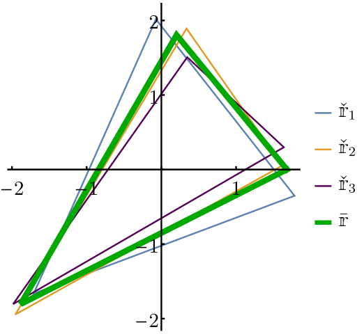
Having defined the appropriate notion of shape difference, we now define the average. Owing to the nontransitivity of alignment,the definition is more involved than might be expected: it is not possible to simply align all the shapes with each other and then do a simple average, because, as stated above, it is typically impossible for even three shapes to be pairwise aligned with each other. Instead, given a time series of simulated shape samples , , we define their average as the shape that minimizes the sum of with the samples22 2 We use to represent the operation of finding the argument which minimizes a function. That is, if , then is the minimum value of . :
| (19) |
Because is defined only up to rotations, this definition of is defined only up to rotation. The rotational degree of freedom can be fixed e.g. by making the first junction point lie on the positive axis. Once a choice of orientation of has been made, the orientation of each sample can be fixed by aligning it with ; we denote this aligned shape sample . This method of averaging is illustrated in Fig. 15. To justify our choice of this method of averaging, we show in the appendix Appendix that it is equivalent to another natural method of averaging.
III.2 Shape variance from simulation run
In addition to the average micelle shape, we have stated that the shape fluctuations can be used to control the micelle’s interactions. The fluctuations are characterized by a variance matrix , defined by
| (20) |
where the tensor product gives the second rank tensor that acts on a shape according to the rule .
These shape fluctuations limit the precision to which the mean shape is determined. Naturally, one wants to be able to quantify this precision. Indeed, to convincingly show that the micelle’s shape depends on its composition, as we indeed set out to do, we must show that the variability in the mean shapes cannot be explained only by the uncertainty caused by the limited precision of the simulation technique. Consequently, it is necessary to estimate this uncertainty in the mean shape. A naive estimate for the variance matrix representing the degree of uncertainty in is . However, this would underestimate the uncertainty since the shape samples are correlated. If the system was described by a single correlation time of sampling intervals, then the correlations could be accounted for by using the estimate . However, to make matters more complicated, there is no single correlation time describing the correlations in the sample. Typically we find large scale cooperative fluctuations have longer correlation times than high wavenumber fluctuations.
To address this complication, we find the autocorrelation time of each fluctuation mode independently, as we now describe in more detail. A mode is an eigenvector of the variance matrix . This eigenvector has a corresponding eigenvalue , so that
| (21) |
(To fix the ordering of the with respect to , we arrange them in decreasing order of .) For each , we define time series of mode amplitudes given by
| (22) |
Under sufficient simplifying assumptions, the mode amplitudes may be used to estimate the uncertainty in , following canonical methods [50]. Specifically, this estimate of uncertainty assumes that the mode amplitudes are sufficiently small that shape fluctuates as a harmonic system in thermal equilibrium and consequently the normal mode amplitudes fluctuate independently. In such a harmonic system each mode has a characteristic autocorrelation time (in units of the sampling interval), which we estimate using the initial convex sequence estimator of [51]. Samples of the amplitude separated by times longer than sampling intervals may be viewed as statistically independent, so that the number of independent samples of the th mode amplitude is . Accordingly, the squared uncertainty in the mean along the direction is estimated to be the variance of the shape distribution along this direction divided by the number of independent samples . We therefore estimate the variance matrix given the uncertainty in the mean by
| (23) |
A graphical representation of an average micelle shape together with its variance and variance in mean is shown in Fig. 16.
Since this uncertainty estimation ignores uncertainties in the mode eigenvectors , and moreover our system’s fluctuations may be too large to permit a harmonic approximation, the estimate of Eq. 23 may be inaccurate. However in Sec. III.5, we will describe a way of validating Eq. 23 by checking whether the expected uncertainty in within a simulation run is consistent with the repeatability of over several simulation runs. Then in Sec. IV.1, we will use this validation to show our results are largely consistent with this harmonic scheme.
III.3 Rejecting malformed micelles
In the case shown in Fig. 16, the diblock junction points make a smooth curve along the surface of the micelle, indicating that the bonds joining the diblocks were sufficient to make the micelle well-formed. However, this is not the case with every simulation. Fig. 17a shows a case where multiple diblock junction points crossed from one side of the micelle to the other. In addition to this example, we have observed cases where the solvophobic region of the micelle splits into two or more disconnected pieces, as shown in Fig. 17b. Since this work is concerned only with the behavior of well-formed micelles, we simply discard any such results where the average micelle shape is malformed.
If data is to be discarded in a consistent manner, a precise definition of “well-formed” is needed. We considered a shape to be well-formed if it satisfies two criteria: an ordering criterion and a smoothness criterion. The ordering criterion is satisfied if the shortest closed path visiting each junction exactly once visits the junction points in the intended order. This criterion detects whether diblocks cross from one side of the micelle surface to another, and it also detects smaller defects such as a transposition of two diblocks. The smoothness criterion is satisfied if the maximum distance between any two sequential junction points exceeds the median distance by less than forty percent. The smoothness criterion detects whether diblocks have broken off from the main surface either to form a small aggregate of diblocks outside the micelle, or form a cluster of solvophilic beads in the interior of the micelle. We found that about half of the average micelle shapes resulting from our simulations satisfied both criteria for being well-formed.
III.4 Combining simulation runs
So far, we have discussed how to determine an average micelle shape and its fluctuation from a single simulation run. However, we performed multiple simulation runs of each micelle with different random initial velocities (see Sec. II.5) to both generate more statistical data, and more crucially to confirm that the uncertainties in each simulation run’s mean shape are well estimated. Therefore, for each micelle composition there is not one, but average shapes, denoted , , and each of these has a corresponding variance and variance in mean . In this section, we describe how these quantities are combined to produce a best estimate of the shape, its fluctuations, and its error. To represent these best estimates, we will use the corresponding symbols, but without the subscript. More explicitly, denotes the combined average; , the combined variance; and , the error in the combined mean.
It would be possible to combine the means via the simple minimization given in Eq. 19. However this formula would ignore the uncertainties in the means. These uncertainties ought to be taken into account, because mean shapes with lower uncertainty should be given more weight in determining the combined mean. Indeed, as might be predicted from the outliers of Fig. 8b, we do find that there is a significant variability in simulation runs’ uncertainties in the mean. To account for the uncertainties, we may define the combined mean using a maximum likelihood estimate [50]. Under the canonical assumptions of a harmonic system in thermal equilibrium, we expect the probability distribution of to be Gaussian, so the log-likelihood of a true average shape given an estimated average and its error is (up to an unimportant constant offset) proportional to following quadratic form:
| (24) |
where is the result of aligning with . Since this log-likelihood depends only on , it is independent of rotations of , as desired. The product in Eq. 24 involving a matrix inversion is indeed well-defined since does have full rank when viewed as an operator on the space of shapes aligned with , and the shapes indeed lie in this space.
Having defined the log-likelihood of a mean given a single simulation, we may now define the same for multiple simulation runs. This is facilitated by the fact that the runs are statistically independent from one another, so that the joint probability of measuring each with the uncertainty given the true mean shape is the product of the individual probabilities, and therefore the log-likelihood of the true mean shape given the and is simply the sum of the individual log-likelihoods. Therefore the maximum likelihood estimate for the true mean shape is given by maximizing the sum of log-likelihoods:
| (25) |
Once the average is found, one can ask what is the best estimate for the fluctuations that can be made from each run’s mean and variance . We make this best estimate by finding the variance matrix which best represents the fluctuations aggregated over all simulation runs. The variance represents a set of samples aligned with . The first step in estimating the variance from the shape samples via Eq. 20 is to align the samples with the mean (in the present case, ).
This alignment can be decomposed into two steps. First we apply to each sample the rotation which aligns with , producing the aligned mean shape given by and the rotated samples , given by . However, the alignment of the sample with the combined mean is not yet complete: although is aligned with , and is aligned with , nontransitivity implies that is typically not aligned with .
An additional, albeit small, rotation specific to each sample is necessary to complete the alignment. If the rotation is to align the sample with , then, by the reasoning found below Eq. 17, we must have , where is defined in Eq. 17 as a counter-clockwise rotation of .
To make progress, we observe that since the misalignment caused by nontransitivity is typically small, and so the required rotation angle is small, we may make the Taylor expansion approximation . Since each sample is near its corresponding mean, we further make the approximation . Combining these two approximations, we find that the action of on the sample is given by
| (26) |
Inserting the approximation into the condition for alignment, we obtain , so that . Inserting this into Eq. 26, we find the action of the second rotation on a sample to be
| (27) |
where we have defined the projection operator to be the tensor in parentheses above. We see that the combined effect of the two rotations on a sampled fluctuation is given by the linear operator . Consequently, the variance matrix for the aligned samples is , which we denote by .
If the aligned fluctuations from each simulation run were aggregated, the resulting variance matrix would be the weighted average of the individual of each run, weighted by the number of samples. However, since each run had approximately the same length, they generate approximately the same number of samples, and so we make the approximation that the best estimate for the combined variance is a simple average of the :
| (28) |
To estimate the variance in the mean giving the uncertainty in , we also perform an average. Just as in Eq. 28, we must revise the original to account for the fact that the best estimate of the mean is now , and to align with this . Accordingly we perform the same alignment transformation on each that was done for the sample variances above. The result is denoted . We then average these values as in Eq. 28. This average doesn’t change systematically as increases. However the overall variance in the mean of independent samples is times this average. Thus
| (29) |
III.5 Testing consistency between simulation runs
At the end of Sec. III.2, we stated that the uncertainties defined by Eq. 23 could be tested by comparing them to the observed variability in the mean shape. Having defined the average , we may use defined in Eq. 24 to measure the differences between the individual run averages and the combined mean . Since is the negative of the chi-squared statistic and each mean has degrees of freedom, we expect that this should be of order . We may therefore define the reduced chi-squared of a combined average by
| (30) |
We expect this to be near unity; however, if the simulation runs were too short so that the full range of thermal shapes is not explored in a single simulation, then the difference in the means would be larger than the errors in the means would suggest, and would be much larger than unity. Thus is a statistic that tests how well-estimated are the uncertainties from each simulation run of a given micelle composition. Since the are defined using (see Eq. 23), the provide an indirect test of the as well.
In fact, it is possible to validate the uncertainties in more detail. From Eq. 23, we expect that the uncertainty of the mean in the direction of its th mode is given by . To verify this expectation, we can define the chi-squared of the th mode by
| (31) |
For each , we expect that should be near unity. Testing this expectation gives a more thorough validation of Eq. 23, and in particular that finding the correlation time of each mode is sufficient to characterize the full correlations of the shape fluctuations. The reduced chi-squared for each micelle composition and a representative set of chi-squareds for the modes of one simulation run are presented in Sec. IV.1.
In addition to testing the formulas for the simulation runs and their uncertainties defined in Sec. III.1 and Sec. III.2, we would like to validate the combined average and its uncertainty . One method of validation is to verify that the result of combining the and the is consistent with the result of first concatenating the list of samples , and then finding a mean from these samples, using Eq. 19 as if the samples were generated from a single simulation. We chose to compare with the average of the combined samples, denoted by , since the procedure for averaging a time series of shapes can itself be validated using and . Once the average of the combined samples has been found, a statistic similar to the one in Eq. 31 can be computed. More precisely, we define by
| (32) |
where is the th eigenmode of and is the associated eigenvalue. An example calculation of this statistic will be presented in Sec. IV.1.
III.6 Shape features
We have now given a complete description about how to extract micelle shape information from the simulation. However, in this paper we will pay special attention to two features of the micelle shape: the “curvature ratio” and the “normalized fluctuation”. The curvature ratio is defined as the ratio of average signed curvature of the micelle surface region occupied by the solvophobic-rich diblocks divided by that of the solvophilic-rich diblocks as illustrated in Fig. 18.
We are interested in this quantity because our intent is to use our shape-design mechanism to produce a micelle of unusual shape, specifically one with a dimple. The curvature ratio quantifies the strength of this dimple, and therefore can help detect the conditions under which our shape-design mechanism works best.
In addition to the average shape, we are interested in the shape fluctuations, as noted previously. We have introduced the variance matrix to characterize the shape fluctuations. We summarize the size of the fluctuations represented by this matrix with a single scalar, the normalized fluctuation , to measure the amount of fluctuation in the micelle shape, normalized so as not to scale with the number of junction points or the size of the micelle. The normalized fluctuation is defined by
| (33) |
It is enlightening to notice a connection between the normalized fluctuation and the distance metric : if and are the mean and variance of a single simulation run, then by Eq. 20 and Eq. 14, the for this simulation run is given by
| (34) |
Since we will be analyzing these two features of micelle shape, we must make an estimate of their uncertainty. The uncertainty of the curvature ratio can be straightforwardly derived from the full variance matrix giving the variance in the mean.
Estimating the uncertainty in the fluctuation is more subtle because is defined in terms of the variance , and so the error in delta represent the error in the fluctuations of a quantity rather than the error in the quantity itself. Consequently, we attempt only a rough estimate to the error in . The dominant source of uncertainty in comes from . We find the uncertainty in by recognizing that the trace is the sum of eigenvalues:
| (35) |
Evidently, it sufficient to estimate the uncertainty in each variance. To perform this estimate, we resort to assuming that each represents the variance of a Gaussian distribution. Given samples of a univariate Gaussian random variable with variance , a formula for the uncertainty of the estimate of the distribution’s variance is given by (see [52])
| (36) |
To use this formula to estimate the uncertainty in , we must choose a value for the number of independent samples contributing to the estimation of . We estimate this number of samples for each mode of , by taking the ratio of the fluctuation in the mode amplitude with the uncertainty in the mean along the direction:
| (37) |
As this estimate of the normalized fluctuation uncertainty requires approximation in the form of Eqs. 36 and 37, some degree of validation is in order. To this end, we calculate the normalized fluctuation from each simulation run (i.e., substitute and in Eq. 33), and compute the standard error in the resulting normalized fluctuations. While this second method may seem reasonable, we prefer the uncertainty estimate described in the preceding paragraphs to the second estimate for two reasons: first, the second estimate cannot be used if there is only one simulation run producing a well-formed micelle; and second, the first estimate is less likely to underestimate the uncertainty because it takes into account all modes while the second estimate can result in an underestimate if the normalized fluctuations from individual happen to be similar. The results of using these two methods is compared in Sec. IV.1.
IV Results
In this section, we present the results of simulating micelles of several compositions. The range of micelle compositions was not chosen to be exhaustive but only to demonstrate a significant degree of control over the micelle shape. To this end, we varied two aspects of the micelle composition: the length of the core chain and the composition of the solvophobic-rich diblocks. The length of the core chain ranged from 600 beads to 1000 beads. Two solvophobic-rich diblock compositions were studied, the first being solvophobic beads and solvophilic beads and the second being solvophobic beads and solvophilic beads. Since the first composition has a larger asymmetry, and therefore the micelles containing these diblocks have a larger asymmetry contrast between their solvophobic-rich and solvophilic-rich diblocks, we refer to these micelles as “high contrast”. Conversely, we refer to the other micelles, whose solvophobic-rich diblocks contain solvophobic beads and solvophilic beads, as “low contrast”. Other aspects of the micelle composition were held constant: each micelle had solvophobic-rich diblocks and solvophilic-rich diblocks, and the solvophilic-rich diblocks each had solvophobic beads and solvophilic beads. To obtain sufficient statistics, each simulation was run in parallel on nine cores for hours, during which time LAMMPS completed about one billion timesteps. The mean shapes, fluctuations, and uncertainties resulting from these simulations are plotted in Table 2.
In Sec. IV.1, we discuss the results of validation tests discussed in Sec. III.5 and Sec. III.6. In Sec. IV.2, we show the average shapes of the micelles, and plot the shape features introduced in Sec. III.6 as a function of the size of the core and the asymmetry ratio of the solvophobic-rich diblocks.
| 600 Core | 700 Core | 848 Core | 1000 Core | |
| high contrast | ||||
| low contrast |
IV.1 Validation of analysis
In Sec. III.5, we introduced two statistics and , defined in Eqs. 30 and 31, for validating that the variation in the means was consistent with the error in these means. We stated that a correctly estimated error leads to the statistics being nearly one, while underestimated error lead to large values and overestimated errors lead to small values. One cause of concern motivating this test is that the simulations may not have been run long enough for the full range of thermal shapes to explore, leading to the estimated mean of a simulation run being strongly biased by the initialization. This would lead to the means being more different than mere thermal fluctuations would predict, and therefore lead to large and . Another cause for concern is that the assumption underpinning Eq. 23, namely that the fluctuation mode amplitudes fluctuate independently and are each described by a separate correlation time may be strongly violated to the point that Eq. 23 gives an unsatisfactory estimate of the uncertainty in the mean. A shortcoming of the estimate Eq. 23 would likely because a systematic dependence of on the mode number , since we expect the applicability our assumptions to depend on the amplitude or correlation of the mode, both of which vary systematically with .
| 600 Core | 700 Core | 848 Core | 1000 Core | |
| high contrast | 5.5 | 0.69 | 1.8 | — |
| low contrast | 59 | 1.2 | 2.3 | 3.2 |
Results for are given in Table 3. The simulations of low contrast micelles having core beads had a large . This happened because two of the four simulations fluctuated only modestly about significantly different, but well-defined mean shapes. The other two of the four simulation runs showed large fluctuations. This suggests that, for this micelle composition, there are multiple metastable shapes between which the micelle can fluctuate. This example demonstrates the benefit of doing multiple independent simulation runs and shows the limitations of representing a shape with a single mean and a variance about the mean.
On the other hand, besides the two aforementioned cases, all the are near unity, indicating that the uncertainty in the mean shape from each run is well-estimated.
Next we consider the of Sec. III.5. A more detailed diagnostic than the , the indicate how well the shape error of the th simulation run in the direction of the th mode is estimated. To give context to the analysis of the , we first show a representative plot of the mode amplitude variances vs , and we show a few modes in Fig. 19.


We find that the mode amplitude variance varies by three orders of magnitude. With this in mind, we plot in Fig. 20 for a representative simulation run of a low contrast micelle with core beads. Although the mode variances and correlation times vary by several orders of magnitude, the remain mostly within their confidence interval with no apparent systematic dependence on , giving a positive validation of the assumptions used to calculate . In particular, this validation gives credence to the form of Eq. 23 used to calculate the error in the mean of a single run, where each mode is assumed to have an independent correlation time estimated by the time series of that mode’s amplitude.
If the correlation times were estimated incorrectly, then the for small would be significantly different than the for large . As an extreme example of an incorrect correlation time estimation, consider the effect of ignoring correlation times completely (i.e., inserting into Eq. 23 as done in Fig. 20): the error in the mean along the high-amplitude modes is underestimated and so the corresponding are much larger than unity. This analysis was done for a single run using one of our more stable compositions. Naturally, less well-behaved micelle compositions and runs, such as the low-contrast composition with 600-bead core, are not expected to fare as well under the same analysis.
Next, in Sec. III.6, we described a way to estimate the uncertainty in the normalized fluctuation by individually estimating the uncertainty in each mode variance . Then, to validate this estimate, we proposed performing a comparison to the standard error of the normalized fluctuations individually calculated from each simulation run. The comparison is shown Fig. 21. We expect only rough agreement because the estimate being validated assumed the shape data is drawn from a Gaussian distribution. In fact the size of the errors are only consistent to about a factor of two. Therefore, when evaluating the significance of the results in Sec. IV.2, it should be remembered that the uncertainties in the normalized fluctuations are determined only to this limited precision.
Finally, we validate the formula Eq. 25 for the combined mean and its uncertainty estimate defined by Eq. 29. This validation is done by comparing the combined mean with the combined set of all shape samples, as described in Sec. II.3. In Fig. 22, we show a plot of the statistic , defined in Eq. 32, for the low contrast micelle with core beads. The fall within the expected range, and the -average of is . The difference between this value and the ideal value of suggests that the error in the combined mean may be slightly underestimated. From Fig. 22, this underestimation seems to be worst for low modes.
IV.2 Shape features
Finally we discuss our findings concerning the shape features discussed in Sec. III.6. To study quantitatively the dependence of micelle shape on composition already apparent in Table 2, we plot in Fig. 23 the curvature ratios and normalized fluctuations of these shapes, as well as a fit to a simple linear model. Several trends are revealed by these plots. The curvature ratio becomes more negative (meaning that the dimple becomes more pronounced) as the asymmetry ratio becomes more negative (meaning the solvophobic-rich diblocks become even more solvophobic). This confirms our intuition explained in Sec. II.4 that the curvature should be positively correlated with the asymmetry ratio.
Another trend is that as the size of the core is increased, the curvature ratio becomes more positive (meaning that the dimple becomes less pronounced). We propose the following explanation for this behavior. We note that an increase in the core size increases the volume of the micelle. This increased volume could be accommodated either by an increase in the perimeter, reducing the density of diblock “surfactant” on the surface and thereby presumably increasing the micelle surface tension, or by making the micelle more circular, thereby making the curvature ratio more positive. In practice, we expect both of these happen to some extent, and so increasing the core size would both increase the surface tension and make the curvature ratio more positive.
The normalized fluctuations are less precisely determined, but trends are still apparent. The data show that the normalized fluctuations decrease as the solvophobic-rich diblocks become more solvophobic. This effect could also be explained in terms of a competition between the preferred perimeter and preferred curvature. As the solvophobic-rich diblocks become more solvophobic, the dimple becomes more pronounced, which we propose leads to an increase in perimeter and consequently surface tension. This increased surface tension would then decrease the amplitude of shape fluctuations. Also, the data suggest that micelles with more core have lower normalized fluctuations, although the size of this effect is on the same order of the uncertainty. We have argued in the previous paragraph that increasing the core should increase surface tension. In addition to reducing the dimple, this increased tension should also reduce fluctuations, explaining the trend.
We note one more feature in the data: the low contrast micelle with has a significantly more positive curvature ratio than the trend line predicts. Although we are not sure how to explain this, we suspect this behavior is related to the onset of a transition reported in [53] involving the buckling a two-dimensional vesicle wall upon decreasing the vesicle’s interior volume. If the energy barrier associated with buckling was high enough to preclude a buckling event from occurring within a simulation, then our observation, previously noted in Sec. IV.1, of two well-defined, but inconsistent micelle shape averages could be explained. In any event, this data point is an interesting starting point for further investigation.
Having described our results, we now note that they afford some degree of predictive power. We have observed a range of curvature ratios with a range extending approximately from to exhibiting a mostly regular dependence of this curvature ratio on micelle composition. Therefore if a micelle with curvature ratio in the observed range is to be constructed, the data provide a way to determine which micelle composition gives the desired curvature ratio. In this way, we have demonstrated that micelle shape design is possible using our design mechanism.
V Discussion
The work presented in this paper is only a first demonstration that our micelle design mechanism can provide for fine control of a micelle shape. In this section, we describe several directions for future exploration: we describe other aspects of micelle composition to vary; we suggest additional features of the thermal shape distribution to control, we suggest a few alternate schemes for bonding the micelle’s constituent diblocks with the idea that they may be more effective at preventing malformed shapes, we propose using a simplified elastic model of the micelle shape energetics, and we discuss how our shape-design strategy might be extended to three dimensions and what challenges may arise. Finally, we discuss how our results are relevant to the applications mentioned in the introduction.
V.1 Further variation of micelle composition
In this work, the effect of only two aspects of micelle composition were studied in this paper, and some speculative explanations of the observed behavior were given. In future work, other aspects of micelle composition may be varied, extending the range of observed micelle shapes and giving further insight into the factors affecting micelle shape. For example, only the asymmetry of the solvophobic-rich diblocks were studied; the effect of varying the solvophilic-rich diblocks could also be studied. Another aspect of the micelle composition to address is the length of the diblocks. In this work, we filled the micelle surface with diblocks of a specific chosen length, and chose the asymmetry of these diblocks to produce the desired curvature. However, there is freedom in choosing the length of the diblocks: the micelle surface could be filled using a larger number of shorter diblocks, holding fixed the imprinted preferred curvature profile. A third way of altering the micelle composition is to introduce another species of diblock. In the micelle shapes presented in Sec. IV, there were three regions of significantly different curvature: the dimple was concave, the surface opposite the dimple was weakly convex, and the surface adjacent the dimple was strongly convex. Since these micelles only contain two species of diblock, the observed micelle shapes seem to be at odds with our stated design strategy, wherein the diblock’s preferred curvature dictates the surface curvature. We expect that the mismatch between the imprinted curvature and the realized curvature represents a frustration which may affect the dynamics (e.g., fluctuations) of the micelle. To test this expectation, one could introduce a third species of diblock to better match the realized micelle curvature, and study the resulting micelle shapes.
V.2 Additional shape features to control
Just as there are many ways to alter the micelle composition, there are many aspects of the micelle shape to control. Here we list three extensions to the shape control demonstrated in this work. First, instead of the curvature ratio of the average shape illustrated in Fig. 18, one could study other quantities characterizing the average shape. In fact, the difference metric , defined in Eq. 14, provides a way of quantifying the similarity to any chosen target shape. Second, we chose a static set of interaction parameters in our model; however, applications may require exposing the micelle to varying environments (having variations of e.g., temperature, pH, or salt concentration). On the one hand, such a varying environment would presumably make it difficult to ensure a fixed micelle shape. On the other hand, there emerges a challenge of designing a micelle that assumes different designed shapes depending on its changing environment. Lastly, we have found evidence of a micelle exhibiting two metastable shapes in a single environment. In this case, there is a breakdown in the representation of the micelle shape as a Gaussian distribution fluctuating about a single mean. Instead, one could categorize the observed micelle shapes into clusters (each representing a metastable micelle shape), and find the mean of each cluster and the transition rates between the clusters. Further, each metastable shape presumably may be designed by changing the micelle composition.
V.3 Avoidance of malformed shapes
Another issue to be addressed in future work is the avoidance of malformed shapes. Although the bond scheme chosen in this work did reduce the occurrence of malformed shapes, it is likely that other bond schemes, while perhaps harder to synthesize, would be even more effective. One could imagine a solvophobic backbone chain with solvophilic (and perhaps solvophobic) side chains; in fact, these bond schemes have been considered theoretically in [11]. Alternatively, the backbone chain could be solvophilic. Even more intricate possibilities are a solvophobic backbone chain with diblock side chains, or even branched side chains where the degree of branching can be used to control the curvature. Examples of alternate bond topologies are shown in Fig. 24. In any case, we imagine that the effect of a diblock’s spontaneous curvature on the shape of a well-formed micelle is mostly independent of the bond scheme used to make the micelle well-formed, so that these two problems may be studied independently.
V.4 Simplified elastic model of micelle shape
Moving beyond particle-based simulations, further insight could be gained by studying a simplified model containing only the physics believed to be necessary to explain the micelle shape (such as the relationship between a diblock’s composition and its preferred curvature), and abstracts away unimportant details (such as the exact nature of the monomer interactions). We have in mind a model where the degrees of freedom are the positions of the junction points, far fewer in number than the positions of each bead. These junctions points would be subject to a potential energy function representing the compression energy of the total volume enclosed by the micelle surface and the energies of surface stretching and bending. However, it is unclear to us if a micelle could faithfully be modeled so simply. Further, if this model is to be useful in experimental applications, the effective parameters of the simple model must somehow be found from the small-scale monomer interactions.
V.5 Extension to three dimensions
Finally, we address the most readily apparent issue: the extension of our design mechanism to three dimensions. We expect the basic principle of our design mechanism—that diblock composition can be used to influence preferred surface and therefore shape—should work similarly in three dimensions. As three dimensional micelles are routinely simulated, we expect that the added computational burden to be minor.


However, there are difficulties that arise in three dimensions. One difficulty is that to lowest order in the curvature, the local bending energy per unit of the micelle surface area is [54] given by
| (38) |
where and are the mean and Gaussian curvatures, is the spontaneous mean curvature, and and are moduli governing the mean and Gaussian curvature, respectively. We expect that the local spontaneous mean curvature parameter ought to depend on the local diblock composition at the surface. Even if this is the case, the local diblock composition determines only one preferred curvature, , but a micelle shape is described by two principal curvatures at each point. Therefore it would seem a micelle shape is underspecified by the mean curvature profile induced by diblocks on the micelle surface. For example, we unduloids [55], a family of distinct shapes all having the same mean curvature profile (examples shown in Fig. 25). The diblocks having mean curvature compatible with the unduloid in Fig. 25b, will likewise have a mean curvature compatible with Fig. 25c, so neither one of these shapes can be designed if diblocks affect only the preferred mean curvature. However, a diblock composition is described by two parameters, a length and an asymmetry ratio, and so it is possible that another parameter in addition to the spontaneous curvature, such as the mean curvature modulus or Gaussian curvature modulus , may be controlled by the diblock composition. In fact this dependence is described theoretically in [35]. This may be sufficient to restore full shape-designability. Alternatively, it is possible that the form of Eq. 38 does not accurately describe the highly curved micelles we consider, because higher order terms in the curvature become relevant; in this case, a preferred Gaussian curvature may arise, allowing for more direct control of the surface curvature. Even if full control of the shape is not possible in three dimensions, it would still be interesting to determine what shape-designability remains.
Another difficulty with extending the shape design mechanism is that a more sophisticated bond scheme is necessary to enforce the relative positioning of the diblocks on the surface of the micelle. Indeed, three-dimensional simulations amphiphilic linear multiblock copolymers and polymers with side chains have been simulated [56], and while rough shape control has been demonstrated, the junction points do not arrange themselves on the micelle surface in an organized manner, so the fine control we seek does not seem possible. Instead, the polymer may need to be realized in the form of a branched polymer. One possibility is to first form a crosslinked polymer network of a roughly spherical shape, and then graft onto the network surface diblocks of the desired compositions. There remains a question of how to create the crosslinked polymer network with chemically distinct surface regions necessary to graft specific species of polymer to specific regions on the surface. We hypothesize that such a network could be created either by growing outward from a multifunctional core such as a silsesquioxane [57] or by growing inward from an external, rigid scaffold such as a protein cage [58]. In either case, after the network is formed, the original core or scaffold could be disassembled, leaving only the flexible polymer network.
V.6 Relevance to applications
We now discuss how our results could be used to address the applications discussed in the introduction. One application was to use shape-designed micelles as drug carriers. It has been found that the carrier shape can affect how much drug can be loaded into the micelle [4]. Also, it has been found that nanoparticle shape can affect where in the body (e.g., in which organ) the particles accumulate [59, 60, 61, 62, 63]. Since we have found it possible to precisely control at least one feature of the micelle shape (presumably more shape features could be controlled with additional effort), one could expect to fully optimize the micelle shape to target a specific organ. Additionally, it was found that carrier shape flexibility affects how quickly the drug is cleared from the body [64, 65, 63, 66]. Our results have demonstrated that this flexibility can be controlled precisely, potentially allowing precise control of drug clearance.
Another application was the lock and key mechanism. In [8], the assembly of concave objects, similar to the ones designed in this work, were studied. It was found that in the presence of depletants, ensembles of these object could be made to aggregate. It was further found that the size of the concave feature affects the aggregation: the concave curvature of the dimple must match the convex curvature of the object to which it will bind. Precise control of the dimple size thereby allows precise control of how these objects aggregate. Additionally, one could imagine that a micelle with large shape fluctuations could deform to fit a wide range of curvature, thus acting as a “master key”. This last possibility highlights the benefits of using diblock copolymer micelles as opposed to more rigid shapes such as proteins.
VI Conclusion
Molecular dynamics simulations were used to study the fluctuating shape of a polymeric micelle at finite temperature in two dimensions. The micelle was constructed from a single, linear, multiblock copolymer. A globular state with the multiblock’s junction points sequentially ordered around the micelle perimeter is often maintained during the course of the simulation when such a state is used as the initial configuration. We demonstrated the effectiveness of a strategy where the multiblock is viewed as a collection of diblock copolymers joined end to end, and the asymmetry of these diblocks is selected to dictate the micelle surface curvature. Specifically, we found that positioning solvophobic-rich diblocks preferring concave curvature on the micelle surface caused the formation of a concave dimple in the surface region occupied by these diblocks. Further, the strength of the dimple is controlled by both the asymmetry of these diblocks, and the size of a homopolymer core chain located in the micelle interior. In addition to the strength of the dimple, the asymmetry of the solvophobic-rich diblocks and the size of the core chain affected the amount of fluctuations in the micelle shape. In future work, the micelle shape design strategy could be studied in three dimensions where it is as yet unclear how precisely polymeric micelles shapes could be controlled.
VII Acknowledgements
The authors thank Juan de Pablo, Greg Voth, Kurt Kremer, and Jeff Vieregg for enlightening conversations regarding the context of this work within the literature and for suggesting modifications to our design scheme to ease experimental realization. We also thank Jian Qin, Steve Tse, James Dama, and Glen Hocky for their guidance in carrying out the simulations presented in this work. This work was completed in part with resources provided by the University of Chicago Research Computing Center. This work was principally supported by the University of Chicago Materials Research Science and Engineering Center, which is funded by the National Science Foundation under award number DMR-1420709.
Appendix Equivalence of two definitions of mean shape
To justify our definition Eq. 19 of , we show that it is equivalent to an alternative notion of average. The alternative definition involves first rotating the shapes so that the summed pairwise square differences are minimized, and then simply taking an arithmetic average. In symbols, we define the minimizing rotation angles by
| (39) |
and then we define the arithmetic average of the shapes by
| (40) |
To transform Eq. 40 into a form more similar to Eq. 19, we use a standard identity relating the expected square differences between two independent samples to expected square difference of a single sample to the mean33 3 Recall if and are two independent, identically distributed random variables, then (using to denote expected value) . This identity applies in our case because is of the form . :
| (41) |
In fact we can proceed further by recognizing that the arithmetic mean minimizes the sum of square differences. Using this fact to transform the right hand side of Eq. 41, we obtain
| (42) |
Using this identity (and ignoring an unimportant multiplicative factor of ), we may transform Eq. 39 into
| (43) |
From this equation, we see that the result from performing a double minimization of with respect to both the and . Now we have already stated above Eq. 42 that the minimizing must be the arithmetic average given by Eq. 40, so that we may simply write
| (44) | ||||
where the second line is obtained by noting that each term in this sum of square differences depends on only one , and the third and fourth lines are obtained by applying the definitions Eq. 14 and Eq. 19 respectively. We conclude that the two notions of average and are indeed the same.
References
- [1] H. Cho, T. C. Lai, K. Tomoda, and G. S. Kwon, AAPS PharmSciTech 16, 10 (2015).
- [2] K. Kataoka, A. Harada, and Y. Nagasaki, Advanced Drug Delivery Reviews 47, 113 (2001).
- [3] A. B. E. Attia, Z. Y. Ong, J. L. Hedrick, P. P. Lee, P. L. R. Ee, P. T. Hammond, and Y.-Y. Yang, Current Opinion in Colloid & Interface Science 16, 182 (2011).
- [4] S. Cai, K. Vijayan, D. Cheng, E. M. Lima, and D. E. Discher, Pharmaceutical Research 24, 2099 (2007).
- [5] S. Venkataraman, J. L. Hedrick, Z. Y. Ong, C. Yang, P. L. R. Ee, P. T. Hammond, and Y. Y. Yang, Advanced Drug Delivery Reviews 63, 1228 (2011).
- [6] E. Fischer, Berichte der deutschen chemischen Gesellschaft 27, 2985 (1894).
- [7] W. Commons, “File:lock and key.png — wikimedia commons, the free media repository,” (2016), [Online; accessed 29-June-2017].
- [8] S. Sacanna, W. T. M. Irvine, P. M. Chaikin, and D. J. Pine, Nature 464, 575 (2010).
- [9] K. Matyjaszewski, Macromolecules 45, 4015 (2012).
- [10] L. M. Bergström, Colloids and Surfaces A: Physicochemical and Engineering Aspects 316, 15 (2008).
- [11] A. R. Khokhlov, A. N. Semenov, and A. V. Subbotin, The European Physical Journal E 17, 283 (2005).
- [12] R. Lipowsky, Advances in Colloid and Interface Science 208, 14 (2014).
- [13] M. C. Watson, E. S. Penev, P. M. Welch, and F. L. H. Brown, The Journal of Chemical Physics 135, 244701 (2011).
- [14] E. Brandt, A. Braun, J. Sachs, J. Nagle, and O. Edholm, Biophysical Journal 100, 2104 (2011).
- [15] R. Goetz, G. Gompper, and R. Lipowsky, Physical Review Letters 82, 221 (1999).
- [16] V. A. Harmandaris and M. Deserno, The Journal of Chemical Physics 125, 204905 (2006).
- [17] M. Hu, J. J. Briguglio, and M. Deserno, Biophysical Journal 102, 1403 (2012).
- [18] P. D. IV and M. Deserno, The Journal of Chemical Physics 138, 214110 (2013).
- [19] M. Laradji and O. G. Mouritsen, The Journal of Chemical Physics 112, 8621 (2000).
- [20] L. Rekvig, B. Hafskjold, and B. Smit, Phys. Rev. Lett. 92, 116101 (2004).
- [21] B. Różycki and R. Lipowsky, The Journal of Chemical Physics 142, 054101 (2015).
- [22] P. Tarazona, E. Chacón, and F. Bresme, The Journal of Chemical Physics 139, 094902 (2013).
- [23] R. M. Venable, F. L. Brown, and R. W. Pastor, Chemistry and Physics of Lipids 192, 60 (2015).
- [24] X. D. Guo, L. J. Zhang, Z. M. Wu, and Y. Qian, Macromolecules 43, 7839 (2010).
- [25] S. M. Loverde, V. Ortiz, R. D. Kamien, M. L. Klein, and D. E. Discher, Soft Matter 6, 1419 (2010).
- [26] N. Poorgholami-Bejarpasi, M. Hashemianzadeh, S. M. Mousavi-khoshdel, and B. Sohrabi, Langmuir 26, 13786 (2010).
- [27] Y. Sheng, X. Yang, N. Yan, and Y. Zhu, Soft Matter 9, 6254 (2013).
- [28] G. Srinivas, D. E. Discher, and M. L. Klein, Nature Materials 3, 638 (2004).
- [29] M. Velinova, D. Sengupta, A. V. Tadjer, and S.-J. Marrink, Langmuir 27, 14071 (2011).
- [30] K. Jelonek, S. Li, X. Wu, J. Kasperczyk, and A. Marcinkowski, International Journal of Pharmaceutics 485, 357 (2015).
- [31] D. Löf, M. Tomšič, O. Glatter, G. Fritz-Popovski, and K. Schillén, The Journal of Physical Chemistry B 113, 5478 (2009).
- [32] R. S. M. Rikken, H. Engelkamp, R. J. M. Nolte, J. C. Maan, J. C. M. van Hest, D. A. Wilson, and P. C. M. Christianen, 7, 12606 EP (2016).
- [33] F. Zhao, J. Sun, Z. Liu, L. Feng, and J. Hu, Journal of Polymer Science Part B: Polymer Physics 48, 364 (2010).
- [34] S. Ljunggren and J. C. Eriksson, J. Chem. Soc., Faraday Trans. 2 85, 1553 (1989).
- [35] Z. Wang and S. A. Safran, The Journal of Chemical Physics 94, 679 (1991).
- [36] J. N. Israelachvili, Intermolecular and Surface Forces, Third Edition, 3rd ed. (Academic Press, 2010) pp. 538–550.
- [37] L. Zhang and A. Eisenberg, Polymers for Advanced Technologies 9, 677 (1998).
- [38] P. L. Golas and K. Matyjaszewski, Chem. Soc. Rev. 39, 1338 (2010).
- [39] F. A. Detcheverry, D. Q. Pike, P. F. Nealey, M. Müller, and J. J. de Pablo, Phys. Rev. Lett. 102, 197801 (2009).
- [40] K. Binder, B. Mognetti, W. Paul, P. Virnau, and L. Yelash, “Computer simulations and coarse-grained molecular models predicting the equation of state of polymer solutions,” in Polymer Thermodynamics: Liquid Polymer-Containing Mixtures, edited by B. A. Wolf and S. Enders (Springer Berlin Heidelberg, Berlin, Heidelberg, 2011) pp. 329–387.
- [41] P. Dimitrakopoulos, Phys. Rev. Lett. 93, 217801 (2004).
- [42] C.-C. Hsieh, S. Jain, and R. G. Larson, The Journal of Chemical Physics 124, 044911 (2006).
- [43] S. Plimpton, Journal of Computational Physics 117, 1 (1995).
- [44] M. Doi and S. Edwards, The Theory of Polymer Dynamics, International series of monographs on physics (Clarendon Press, 1988) p. 151.
- [45] M. Doi and S. Edwards, The Theory of Polymer Dynamics, International series of monographs on physics (Clarendon Press, 1988) p. 11.
- [46] J. R. Rumble, ed., CRC Handbook of Chemistry and Physics, 98th Edition (CRC Press/Taylor & Francis, Boca Raton, FL, 2018) pp. 13–21–13–25.
- [47] G. Wypych, in Handbook of Polymers (Second Edition) (ChemTec Publishing, 2016) second edition ed., pp. 340 – 344.
- [48] L. J. Fetters, D. J. Lohse, and R. H. Colby, “Chain dimensions and entanglement spacings,” in Physical Properties of Polymers Handbook, edited by J. E. Mark (Springer New York, New York, NY, 2007) pp. 447–454.
- [49] K. Lewandowski and M. Banaszak, Journal of Non-Crystalline Solids 355, 1289 (2009).
- [50] P. R. Bevington and D. K. Robinson, Data reduction and error analysis for the physical sciences; 3rd ed. (McGraw-Hill, New York, NY, 2003).
- [51] S. Brooks, A. Gelman, G. Jones, and X. Meng, Handbook of Markov Chain Monte Carlo, Chapman & Hall/CRC Handbooks of Modern Statistical Methods (CRC Press, 2011) p. 16.
- [52] C. R. Rao, Linear statistical inference and its applications, 2nd ed., Wiley series in probability and mathematical statistics (Wiley, New York, 1973) p. 438.
- [53] S. Leibler, R. R. P. Singh, and M. E. Fisher, Phys. Rev. Lett. 59, 1989 (1987).
- [54] W. Helfrich, Z. Naturforsch 28, 693 (1973).
- [55] C. Delaunay, Journal de Mathématiques Pures et Appliquées , 309 (1841).
- [56] V. V. Vasilevskaya and V. A. Ermilov, Polymer Science Series A 53, 846 (2011).
- [57] D. B. Cordes, P. D. Lickiss, and F. Rataboul, Chemical Reviews 110, 2081 (2010).
- [58] M. J. Abedin, L. Liepold, P. Suci, M. Young, and T. Douglas, Journal of the American Chemical Society 131, 4346 (2009).
- [59] P. Decuzzi, B. Godin, T. Tanaka, S.-Y. Lee, C. Chiappini, X. Liu, and M. Ferrari, Journal of Controlled Release 141, 320 (2010), pharmaceutical Nanotechnology: Unmet Needs in Drug Delivery.
- [60] P. V. Devarajan, A. B. Jindal, R. R. Patil, F. Mulla, R. V. Gaikwad, and A. Samad, Journal of Pharmaceutical Sciences 99, 2576 (2010).
- [61] S. Muro, C. Garnacho, J. A. Champion, J. Leferovich, C. Gajewski, E. H. Schuchman, S. Mitragotri, and V. R. Muzykantov, Molecular Therapy 16, 1450 (2008).
- [62] R. R. Patil, R. V. Gaikwad, A. Samad, and P. V. Devarajan, Journal of Biomedical Nanotechnology 4, 359 (2008).
- [63] E. R. Gillies, E. Dy, J. M. J. Fréchet, and F. C. Szoka, Molecular Pharmaceutics 2, 129 (2005), pMID: 15804187.
- [64] B. Chen, K. Jerger, J. M. Fréchet, and F. C. Szoka, Journal of Controlled Release 140, 203 (2009), proceedings of the Fourtheenth International Symposium on Recent Advances in Drug Delivery Systems.
- [65] M. E. Fox, F. C. Szoka, and J. M. J. Fréchet, Accounts of Chemical Research 42, 1141 (2009).
- [66] C. C. Lee, M. Yoshida, J. M. J. Fréchet, E. E. Dy, and F. C. Szoka, Bioconjugate Chemistry 16, 535 (2005).
