Autonomous Dynamical System Approach for Inflationary Gauss-Bonnet Modified Gravity
Abstract
In this paper we shall analyze the gravity phase space, in the case that the corresponding dynamical system is autonomous. In order to make the dynamical system autonomous, we shall appropriately choose the independent variables, and we shall analyze the evolution of the variables numerically, emphasizing on the inflationary attractors. As we demonstrate, the dynamical system has only one de Sitter fixed point, which is unstable, with the instability being traced in one of the independent variables. This result holds true both in the presence and in the absence of matter and radiation perfect fluids. We argue that this instability could loosely be viewed as an indication of graceful exit in the theory of gravity.
has only
pacs
95.35.+d, 98.80.-k, 98.80.Cq, 95.36.+xI Introduction
The dark energy and the dark matter problem are two of the main unanswered problems in modern theoretical cosmology. The dark energy refers to the late-time acceleration that our Universe is currently experiencing, which was observed in the late 90’s, [1] and it is unarguably the most intriguing problem for current and future theoretical research. The dark matter problem is bit older, and the most popular explanation comes from particle physics, in the context of which, dark matter is materialized by a non-interacting particle, see for example [2], for a deep analysis of various aspects of dark matter candidates. Both the aforementioned problems find appealing theoretical explanations in the context of modified gravity, in it’s various aspects, see the reviews [3, 4, 5, 6], for extensive presentations on the subject. Also, a recently proposed theory that may successfully mimic dark matter in a geometric way, is offered by mimetic theories of gravity [7], see [8] for a recent review.
Among the various modified gravity proposals that exist in the literature, an appealing proposal is Gauss-Bonnet gravity, where is the Gauss-Bonnet invariant. The latter, in four dimensions, is defined as , and with , are the Ricci tensor and the Riemann tensor respectively. From the mathematical form of the Gauss-Bonnet invariant, it is obvious that such a theory could contain higher derivatives, which would render the theory not so appealing, since it would be hard to tackle with. However, although this is true in principle, in the case, the resulting picture turns out that it is greatly simplified in four dimensions, since the theory contains second order derivatives, hence it can be studied more easily than initially one may think. In the context of it is possible to describe various cosmological evolutions [9], like late-time acceleration or the unification of inflation with late-time acceleration [10, 11, 12, 13, 14, 15]. Apart from the inflationary paradigm, several proposals exist for the description of bouncing cosmologies in the context of modified gravity, see for example [16, 17, 18, 19, 20].
In this paper the focus is on the dynamical system corresponding to gravity. Particularly, we shall be interested in providing an autonomous dynamical system analysis, as this was performed in Ref. [21]. In the literature there exist various studies on the subject in the context of Einstein-Hilbert or modified gravity, see for example [22, 23, 24, 25, 26, 27, 28, 29, 30, 31, 32, 33, 34, 35, 36, 37, 38, 39, 40, 41], and also [42], in which an autonomous dynamical system approach was also informally used. The question that naturally springs to mind is why we should use an autonomous dynamical system approach in the first place. The answer to this comes from the fact that for a non-autonomous dynamical system, finding the fixed points may not suffice or maybe one could be lead to not correct conclusions, regarding the phase space. Particularly, the stability of the dynamical system is not guaranteed by solely using theorems like the Hartman-Grobman, which describe autonomous dynamical systems. In order to further support our claim, let us exemplify it by using a characteristic example, which can be found in [43, 21]: Consider the one dimensional dynamical system , the solution of which is, . By looking the solution, it can easily be seen that all the solutions (for the various initial conditions, which have impact on ) tend to for . However, if the standard fixed point analysis of non-autonomous dynamical systems is applied in this case, it yields the result that the only fixed point is , which is not a solution to the dynamical system. In addition, by using standard non-autonomous approaches, it can be found that the vector field is deflected from the solution , which is not correct as we discussed earlier. Hence, in many cases, the non-autonomous dynamical systems analysis may not suffice, so the autonomous dynamical system analysis is compelling.
In view of the above, the purpose of this paper is to provide a dynamical system analysis of the modified gravity theory, focusing on inflationary attractors. We shall provide the general form of the gravity autonomous dynamical system, in the presence of cold matter and radiation, and we shall analyze in detail the dynamical system, focusing on inflationary attractors. The time dependence of the resulting dynamical system is solely contained in the parameter , which is equal to , where is the Hubble rate. Hence, we shall assume that this parameter takes constant-values, and therefore the dynamical system turns out to be autonomous. We shall be particularly interested in the case , which corresponds to the de Sitter vacuum. We shall find the fixed points of the autonomous dynamical system and we shall examine the stability. Also we shall investigate numerically the evolution of the dynamical variables, in terms of the -foldings number, focusing on values in the range , which are more interesting when inflationary theories are considered. As we demonstrate, in all the cases, an unstable de Sitter attractor exists, which may reflect the possibility of having an intrinsic mechanism for the graceful exit in theories.
Before we start our presentation, let us briefly present the geometric framework we shall use, which will be a flat Friedmann-Robertson-Walker (FRW) metric, with line element,
| (1) |
with being the scale factor.
II Autonomous Dynamical System of the Gravity
In this section we shall present in brief some basic features of gravity, and we shall investigate how to construct an autonomous dynamical system by using the cosmological equations and some appropriately chosen variables.
The gravitational action is equal to [10, 11, 12, 13, 14]:
| (2) |
and upon variation with respect to the metric tensor , the gravitational equations of motion are,
| (3) | ||||
It is notable that the equations of motion Eq. (3) do not contain any higher derivative terms. For the flat FRW metric of Eq. (1), the gravitational equations take the following form,
| (4) | ||||
where the “dot” denotes differentiation with respect to the cosmic time, and stand for the energy density of the baryonic matter and radiation respectively. Finally, in Eq. (4) stands for,
| (5) |
Also, for the flat FRW Universe of Eq. (1), the Gauss-Bonnet invariant , takes the following form,
| (6) |
By using the cosmological equations (4), we shall construct a dynamical system that can be rendered autonomous, if a set of appropriately chosen variables is used, and to this end we introduce the following variables,
| (7) |
It is more convenient for the purposes of this paper to use the -foldings number, so by using the following differentiation rule,
| (8) |
and by taking the first derivative of the variables (7), in conjunction with Eqs. (4), after some algebra we obtain,
| (9) | ||||
where the parameter stands for,
| (10) |
The only time-dependence (-dependence) of the dynamical system is contained on the parameter , which we shall assume that it is constant and particularly equal to zero. As we shall see, this case describes a quasi de Sitter evolution, so the phase space analysis will characterize inflationary attractors. Also, since we are interested on inflationary attractors, we shall assume that the -foldings number takes values in the range .
A useful quantity that will make clear the physical significance of the fixed points of the dynamical system, is the effective equation of state parameter (EoS), which is defined as follows,
| (11) |
so by using the definition of the parameter from Eq. (7) and also the definition of the Gauss-Bonnet invariant from Eq. (6), the EoS can be written as follows,
| (12) |
By having the dynamical system of Eq. (9) at hand, and also the EoS (12), in the next section we shall investigate the inflationary phase space of gravity, and we shall analyze numerically the stability of the fixed points.
III Analysis of the Gravity Inflationary Phase Space
Now let us focus on the study of the dynamical system (9), and as we already discussed, the parameter is the only time-dependent parameter in the dynamical system. We shall assume that the value of is zero, in which case the general form of the scale factor that realizes the case, has the following form,
| (13) |
which in general describes a de Sitter evolution. Notice that by fixing , the dynamical system contains parameters which remain general, so in the rest of this section we shall examine the impact of the value on the dynamical system.
Before getting into the details of the analysis, let us briefly present some standard features of dynamical systems analysis, also found in Ref. [43]. Particularly, we shall be interested in the linearization method and the Hartman-Grobman theorem. The latter determines the stability of the fixed points, when this is hyperbolic. Assume that the function is a solution to the following dynamical system,
| (14) |
where is a locally Lipschitz continuous map . We denote with , the fixed points of the dynamical system (14), and also let be the corresponding Jacobian matrix. The latter is equal to,
| (15) |
The Jacobian matrix should be calculated at the fixed points, and the corresponding eigenvalues must satisfy , in order to have a concrete idea on the stability of the fixed points. Assume that the spectrum of the eigenvalues of , is , then a hyperbolic fixed point satisfies . The Hartman theorem, when applied for a autonomous system, indicates the certain existence of a homeomorphic map , with being an open neighborhood of the fixed point , which satisfies . The flow generated by the homeomorphism , is,
| (16) |
which is topologically equivalent to the one appearing in (14). By applying the Hartman theorem, the dynamical system (14), can be written in the following way,
| (17) |
with being a smooth map . Hence, if the Jacobian matrix satisfies , and in addition, if the following holds true,
| (18) |
the fixed point of the dynamical flow , is also a fixed point of the flow (17), and moreover, it is asymptotically stable. Hence, when a hyperbolic fixed point is met, the above statements hold true, and in the converse case, further analysis, supported by numerical studies, are required in order to reveal the stability of the fixed points. This is in fact our strategy, since the resulting fixed points for the gravity, are not hyperbolic.
So let us fix , and we proceed to the study of the dynamical system. For the dynamical system of Eq. (9), the matrix reads,
| (19) |
where in this case, the functions are,
| (20) | ||||
We can easily calculate the fixed points of the dynamical system (9), which for general are,
| (21) | ||||
and in the case , the fixed points coincide and we thus have only the following fixed point,
| (22) |
The corresponding eigenvalues for the fixed point are , so it is not hyperbolic for sure, and as we will demonstrate it is also strongly unstable. Before proceeding to the numerical analysis, let us reveal the physical significance of the fixed point , and to this end let us investigate the behavior of the EoS for the fixed point . So for , the EoS (12) becomes , and in effect, the fixed point is a de Sitter fixed point.
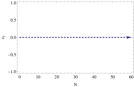
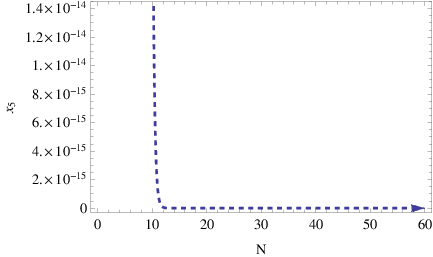
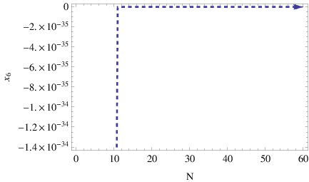
The instability of the fixed point can be revealed only numerically, since the Hartman-Grobman theorem does not apply in our case, due to the fact that the fixed point is not hyperbolic, so by solving numerically the dynamical system (9) for various initial conditions, we can conclude whether the de Sitter fixed point is stable or not. We emphasize our analysis for values of the -foldings in the range , and in Figs. 1 and 2 we plot the numerical solutions for the dynamical system (9),by using the initial conditions , and , , , .
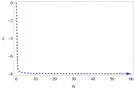
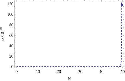
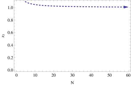
As it can be seen in Fig. 1, the variable tends to quite fast, and also , while , so the de Sitter fixed point is reached, when the parameter is taken into account, while does not converge to zero. From Fig. 2, it can be seen that the variables and tend to their de Sitter values, however the variable tends to zero around . Hence it is obvious that the de Sitter fixed point is not eventually reached from all the variables, and therefore it is an unstable fixed point.
Now let us turn our focus on the purely vacuum case, for which . Actually, the fixed point has features of a vacuum fixed point since , but we shall investigate separately the two cases for clarity.
In the case that matter and radiation are excluded, the dynamical system (9), takes the following form,
| (23) | ||||
and the corresponding matrix becomes in this case,
| (24) |
and in this case, the functions are,
| (25) | ||||
The corresponding fixed point in the case is as expected,
| (26) |
From a physical point of view, the dynamical evolution is qualitatively the same with the scenario we described in the non-vacuum case, due to the fact that . This can be verified by a numerical analysis which we omit for brevity. Hence, the de Sitter fixed point exists in this case too, and it is unstable. In order to further support this result, we shall present another aspect of our numerical analysis, emphasizing in the dynamical system which corresponds to . In this case, the dynamical system becomes,
| (27) | ||||
and in Fig. 3, we present the behavior of the reduced system in terms of the variables . In the left plot, the vector field flow appears, in the plane, while in the right plot, the behavior of various trajectories appear in the plane. As it can be seen in this case too, the reduced system is unstable at , which is the value of the variable at the fixed point in Eq. (26).
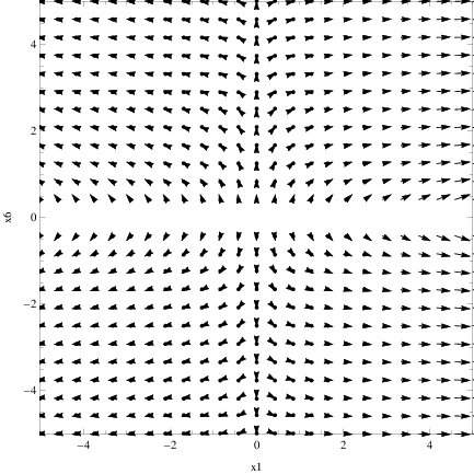
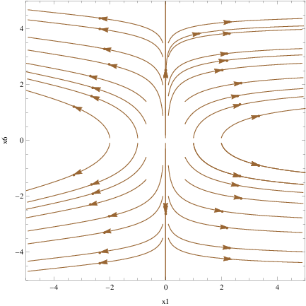
Hence, the autonomous dynamical system (9) both in the vacuum and in the presence of radiation and matter, has a de Sitter fixed point, which is unstable. The instability is mainly caused by the parameter , since it never reaches its fixed point value , and as it seen by the plots in Fig. 3, the dynamical system trajectories and flow are repelled away from the value . This instability could be an indicator of a graceful exit from inflation mechanism inherent in the gravity, both in the vacuum and non-vacuum cases, however a closer analysis on this is required, which we hope to address in a future work.
IV Conclusions
In this paper we performed a detailed numerical analysis of the gravity phase space, in the case that the corresponding dynamical system can be formed to be an autonomous dynamical system. As we demonstrated, by appropriately choosing the free independent variables, the dynamical system can be an autonomous dynamical system, with the only time-dependence being contained in the parameter . We focused on the case , which describes a quasi-de Sitter evolution in the most general case, and we investigated how the dynamical evolution behaves in this case. As we demonstrated, the dynamical system has a de Sitter fixed point, for which the EoS is , and we examined the behavior of the variables numerically. The resulting picture indicated that the fixed point is unstable, a feature that could possibly indicate that the gravity has an inherent instability mechanism, traced on the instability of the variable , which may be seen as a graceful exit from inflation mechanism. This feature however, needs closer inspection, which we plan to do in a future work. Finally, it would be interesting to combine the dynamical system study with the Noether symmetry approach, see for example [44] for a Gauss-Bonnet theory account.
References
- [1] A. G. Riess et al. [Supernova Search Team], Astron. J. 116 (1998) 1009 [astro-ph/9805201].
- [2] V. K. Oikonomou, J. D. Vergados and C. C. Moustakidis, Nucl. Phys. B 773 (2007) 19 doi:10.1016/j.nuclphysb.2007.03.014 [hep-ph/0612293].
- [3] S. Nojiri, S. D. Odintsov and V. K. Oikonomou, Phys. Rept. 692 (2017) 1 doi:10.1016/j.physrep.2017.06.001 [arXiv:1705.11098 [gr-qc]].
- [4] S. Nojiri, S.D. Odintsov, Phys. Rept. 505, 59 (2011);
- [5] S. Nojiri, S.D. Odintsov, eConf C0602061, 06 (2006) [Int. J. Geom. Meth. Mod. Phys. 4, 115 (2007)].
- [6] S. Capozziello, M. De Laurentis, Phys. Rept. 509, 167 (2011);
- [7] A. H. Chamseddine and V. Mukhanov, JHEP 1311 (2013) 135 doi:10.1007/JHEP11(2013)135 [arXiv:1308.5410 [astro-ph.CO]].
- [8] L. Sebastiani, S. Vagnozzi and R. Myrzakulov, Adv. High Energy Phys. 2017 (2017) 3156915 doi:10.1155/2017/3156915 [arXiv:1612.08661 [gr-qc]].
- [9] B. Li, J. D. Barrow and D. F. Mota, Phys. Rev. D 76 (2007) 044027 doi:10.1103/PhysRevD.76.044027 [arXiv:0705.3795 [gr-qc]].
- [10] S. Nojiri and S. D. Odintsov, Phys. Lett. B 631 (2005) 1 [hep-th/0508049].
- [11] S. Nojiri, S. D. Odintsov and O. G. Gorbunova, J. Phys. A 39 (2006) 6627 [hep-th/0510183].
- [12] G. Cognola, E. Elizalde, S. Nojiri, S. D. Odintsov and S. Zerbini, Phys. Rev. D 73 (2006) 084007 [hep-th/0601008].
- [13] E. Elizalde, R. Myrzakulov, V. V. Obukhov and D. Saez-Gomez, Class. Quant. Grav. 27 (2010) 095007 [arXiv:1001.3636 [gr-qc]].
- [14] K. Izumi, Phys. Rev. D 90 (2014) no.4, 044037 [arXiv:1406.0677 [gr-qc]].
- [15] V. K. Oikonomou, Astrophys. Space Sci. 361 (2016) no.7, 211 doi:10.1007/s10509-016-2800-6 [arXiv:1606.02164 [gr-qc]].
- [16] V. K. Oikonomou, Phys. Rev. D 92 (2015) no.12, 124027 doi:10.1103/PhysRevD.92.124027 [arXiv:1509.05827 [gr-qc]].
- [17] A. Escofet and E. Elizalde, Mod. Phys. Lett. A 31 (2016) no.17, 1650108 doi:10.1142/S021773231650108X [arXiv:1510.05848 [gr-qc]].
- [18] A. N. Makarenko and A. N. Myagky, Int. J. Geom. Meth. Mod. Phys. 14 (2017) no.10, 1750148 doi:10.1142/S0219887817501481 [arXiv:1708.03592 [gr-qc]].
- [19] J. Haro, A. N. Makarenko, A. N. Myagky, S. D. Odintsov and V. K. Oikonomou, Phys. Rev. D 92 (2015) no.12, 124026 doi:10.1103/PhysRevD.92.124026 [arXiv:1506.08273 [gr-qc]].
- [20] K. Bamba, A. N. Makarenko, A. N. Myagky and S. D. Odintsov, Phys. Lett. B 732 (2014) 349 doi:10.1016/j.physletb.2014.04.004 [arXiv:1403.3242 [hep-th]].
- [21] S. D. Odintsov and V. K. Oikonomou, arXiv:1711.02230 [gr-qc].
- [22] C. G. Boehmer and N. Chan, doi:10.1142/9781786341044.0004 arXiv:1409.5585 [gr-qc].
- [23] C. G. Boehmer, T. Harko and S. V. Sabau, Adv. Theor. Math. Phys. 16 (2012) no.4, 1145 doi:10.4310/ATMP.2012.v16.n4.a2 [arXiv:1010.5464 [math-ph]].
- [24] N. Goheer, J. A. Leach and P. K. S. Dunsby, Class. Quant. Grav. 24 (2007) 5689 doi:10.1088/0264-9381/24/22/026 [arXiv:0710.0814 [gr-qc]].
- [25] G. Leon and E. N. Saridakis, JCAP 1504 (2015) no.04, 031 doi:10.1088/1475-7516/2015/04/031 [arXiv:1501.00488 [gr-qc]].
- [26] J. Q. Guo and A. V. Frolov, Phys. Rev. D 88 (2013) no.12, 124036 doi:10.1103/PhysRevD.88.124036 [arXiv:1305.7290 [astro-ph.CO]].
- [27] G. Leon and E. N. Saridakis, Class. Quant. Grav. 28 (2011) 065008 doi:10.1088/0264-9381/28/6/065008 [arXiv:1007.3956 [gr-qc]].
- [28] J. C. C. de Souza and V. Faraoni, Class. Quant. Grav. 24 (2007) 3637 doi:10.1088/0264-9381/24/14/006 [arXiv:0706.1223 [gr-qc]].
- [29] A. Giacomini, S. Jamal, G. Leon, A. Paliathanasis and J. Saavedra, Phys. Rev. D 95 (2017) no.12, 124060 doi:10.1103/PhysRevD.95.124060 [arXiv:1703.05860 [gr-qc]].
- [30] G. Kofinas, G. Leon and E. N. Saridakis, Class. Quant. Grav. 31 (2014) 175011 doi:10.1088/0264-9381/31/17/175011 [arXiv:1404.7100 [gr-qc]].
- [31] G. Leon and E. N. Saridakis, JCAP 1303 (2013) 025 doi:10.1088/1475-7516/2013/03/025 [arXiv:1211.3088 [astro-ph.CO]].
- [32] T. Gonzalez, G. Leon and I. Quiros, Class. Quant. Grav. 23 (2006) 3165 doi:10.1088/0264-9381/23/9/025 [astro-ph/0702227].
- [33] A. Alho, S. Carloni and C. Uggla, JCAP 1608 (2016) no.08, 064 doi:10.1088/1475-7516/2016/08/064 [arXiv:1607.05715 [gr-qc]].
- [34] S. K. Biswas and S. Chakraborty, Int. J. Mod. Phys. D 24 (2015) no.07, 1550046 doi:10.1142/S0218271815500467 [arXiv:1504.02431 [gr-qc]].
- [35] D. Müller, V. C. de Andrade, C. Maia, M. J. Rebouças and A. F. F. Teixeira, Eur. Phys. J. C 75 (2015) no.1, 13 doi:10.1140/epjc/s10052-014-3227-2 [arXiv:1405.0768 [astro-ph.CO]].
- [36] B. Mirza and F. Oboudiat, Int. J. Geom. Meth. Mod. Phys. 13 (2016) no.09, 1650108 doi:10.1142/S0219887816501085 [arXiv:1412.6640 [gr-qc]].
- [37] S. Rippl, H. van Elst, R. K. Tavakol and D. Taylor, Gen. Rel. Grav. 28 (1996) 193 doi:10.1007/BF02105423 [gr-qc/9511010].
- [38] M. M. Ivanov and A. V. Toporensky, Grav. Cosmol. 18 (2012) 43 doi:10.1134/S0202289312010100 [arXiv:1106.5179 [gr-qc]].
- [39] M. Khurshudyan, Int. J. Geom. Meth. Mod. Phys. 14 (2016) no.03, 1750041. doi:10.1142/S0219887817500414
- [40] R. D. Boko, M. J. S. Houndjo and J. Tossa, Int. J. Mod. Phys. D 25 (2016) no.10, 1650098 doi:10.1142/S021827181650098X [arXiv:1605.03404 [gr-qc]].
- [41] L. N. Granda and D. F. Jimenez, arXiv:1710.07273 [gr-qc].
- [42] S. D. Odintsov and V. K. Oikonomou, Phys. Rev. D 93 (2016) no.2, 023517 doi:10.1103/PhysRevD.93.023517 [arXiv:1511.04559 [gr-qc]].
- [43] Stephen Wiggins, Introduction to Applied Nonlinear Dynamical Systems and Chaos, Springer, New York, 2003
- [44] S. Capozziello, M. De Laurentis and S. D. Odintsov, Mod. Phys. Lett. A 29 (2014) no.30, 1450164 doi:10.1142/S0217732314501648 [arXiv:1406.5652 [gr-qc]].