One-pass Person Re-identification by
Sketch Online Discriminant Analysis
Abstract
Person re-identification (re-id) is to match people across disjoint camera views in a multi-camera system, and re-id has been an important technology applied in smart city in recent years. However, the majority of existing person re-id methods are not designed for processing sequential data in an online way. This ignores the real-world scenario that person images detected from multi-cameras system are coming sequentially. While there is a few work on discussing online re-id, most of them require considerable storage of all passed data samples that have been ever observed, and this could be unrealistic for processing data from a large camera network. In this work, we present an one-pass person re-id model that adapts the re-id model based on each newly observed data and no passed data are directly used for each update. More specifically, we develop an Sketch online Discriminant Analysis (SoDA) by embedding sketch processing into Fisher discriminant analysis (FDA). SoDA can efficiently keep the main data variations of all passed samples in a low rank matrix when processing sequential data samples, and estimate the approximate within-class variance (i.e. within-class covariance matrix) from the sketch data information. We provide theoretical analysis on the effect of the estimated approximate within-class covariance matrix. In particular, we derive upper and lower bounds on the Fisher discriminant score (i.e. the quotient between between-class variation and within-class variation after feature transformation) in order to investigate how the optimal feature transformation learned by SoDA sequentially approximates the offline FDA that is learned on all observed data. Extensive experimental results have shown the effectiveness of our SoDA and empirically support our theoretical analysis.
Index Terms:
Online learning, Person re-identification, Discriminant feature extractionI Introduction
Person re-identification (re-id) [51, 1, 13, 22, 31, 20, 54] is crucially important for successfully tracking people in a large camera network. It is to match the same person’s images captured at non-overlapping camera views at different time. Person re-id by visual matching is inherently challenging because of the existence of many visually similar persons and dramatic appearance changes of the same person caused by the serious cross-camera-view variations such as illumination, viewpoint, occlusions and background clutter. Recently, a large number of works [22, 23, 3, 16, 27, 30, 35, 44, 53] have been reported to solve this challenge.
However, it is largely unsolved to perform online learning for person re-identification, since most person re-id models except [25, 39, 29, 37] are only suitable for offline learning. On one hand, the offline learning mode cannot enable a real-time update of person re-id model when a large amount of persons are detected in a camera network. An online update is important to keep the cross-view matching system work on recent mostly interested persons, that is to make the whole re-id system work on sequential data. On the other hand, online learning is helpful to alleviate the large scale learning problem (either with high-dimensional feature, or on large-scale data set, or both) nowadays. By using online learning, especially the one-pass online learning, it is not necessary to always store (all) observed/passed data samples.
In this paper, we overcome the limitation of offline person re-id methods by developing an effective online person re-id model. We proposed to embed the sketch processing into Fisher discriminant analysis (FDA), and the new model is called Sketch online Discriminant Analysis (SoDA). In SoDA, the sketch processing preserves the main variations of all passed data samples in a low-rank sketch matrix, and thus SoDA enables selecting data variation for acquring discriminant features during online learning. SoDA enables the newly learned discriminant model to embrace information from a new coming data sample in the current round and meanwhile retain important information learned in previous rounds in a light and fast manner without directly saving any passed observed data samples and keeping large-scale covariance matrices, so that SoDA is formed as an one-pass online adaptation model. While no passed data samples are saved in SoDA, we propose to estimate the within-class variation from the sketch information (i.e. a low-rank sketch matrix), and thus in SoDA an approximate within-class covariance matrix can be derived. We have provided in-depth theoretical analysis on how sketch affects the discriminant feature extraction in an online way. The rigorous upper and lower bounds on how SoDA approaches its offline model (i.e. the classical Fisher Discriminant Analysis [41]) are presented and proved.
Compared to existing online models for person re-id [25, 39, 29, 37], SoDA is succinct, but it is theoretically guaranteed and effective. While most existing online re-id models have to retain all observed passed data samples, the proposed SoDA relies on the sketch information from historical data without any explicit storage of passed data samples, and sketch information will assist our online model in preventing one-pass online model from being biased by a new coming data. While a more conventional way for online learning of FDA is to update both within-class and between-class covariance matrices directly [33, 48, 38, 26, 34, 15], we introduce a novel approach to realize online FDA by mining any within-class information from a sketch data matrix, and this provides a lighter, more effecient and effective online learning for FDA. We also find that an extra benefit of embedding sketch processing in SoDA is to simultaneously embed dimension reduction as well, so that no extra learning task on learning dimension reduction technology (e.g. PCA) is required and SoDA is more flexible when learning on some high dimensional data [22, 5] in an online manner.
We have conducted extensive experiments on three largest scale person re-identification datasets in order to evaluate the effectiveness of SoDA for learning person re-identification model in an online way. Extensive experiments are also included for comparing SoDA with related online learning models, even though they were not applied to person re-identification before.
The rest of the paper is organized as follows. In Sec. II, the related literatures are first reviewed. We elaborate our online algorithm and analyze the space and time complexity of SoDA in Sec. III. Then we present theoretical analysis on the relationship between our SoDA and the offline FDA in Sec. IV. Experimental results for evaluation and verification of our theoretical analysis are reported in Sec. V and finally we conclude the work in Sec. VI.
II Related Work
Online Person re-identification. While person re-identification has been investigated in a large number of works [51, 1, 13, 31, 20, 54, 22, 23, 3, 16, 27, 30, 35, 44, 53, 32, 28, 47], the majority of them only address by offline learning. That is person re-id model is learned on a fixed training dataset. This ignores the increase demand of data from a visual surveillance system, since thousands of person images are captured day by day and it is demanded to train a person re-id system on streaming data so as to keep the system update to date.
Recently, only a few works [37, 25, 39, 29] have been developed towards online processing for person re-identification. The most related work is the incremental distance metric based online learning mechanism (OL-IDM) proposed in [37]. For updating the KISSME metric [17], the OL-IDM utilizes the modified Self-Organizing Incremental Neural Network (SOINN) [8] to produce two pairwise sets: a similar pairs set and a dissimilar pairs set. Although SOINN enables learning KISSME [17] on sequential data, SOINN has to compare the newly observed sample with all the preserved nodes and adds the newly observed sample as a new node if it does not appear in the network. This would be costly as sequential data increase and when feature dimension is high.
Another related work is the human-in-the-loop ones [39, 25, 29], which proposed incremental method learned with the involvement of humans’ feedback. Wang et al. [39] assumes that an operator is available to scan the rank list provided by the proposed algorithm when matching a new probe sample with existing observed gallery ones, and this operator will select the true match, strong-negative match, and weak-negative match for the probe. After having the human feedback, the algorithm is able to be update. Martinel et al. presented a graph-based approach to exploit the most informative probe-gallery pairs for reducing human efforts and developed an incremental and iterative approach based on the feedback [29].
Unlike these models, we design a sketch FDA model called SoDA for one-pass online learning, without any storage of passed observed samples, maintaining a small size sketch matrix on handling streaming data so that the discriminant projections can be updated efficiently for extracting discriminative features for identifying different individuals.
Thanks to the sketch matrix, our SoDA is capable of obtaining comparable performance with offline FDA models on streaming data or large and high dimensional datasets with very low cost on space and time. Compared to the related online person re-id models, SoDA is theoretically sounded since the bounds on approximating the offline model is provided.
In particular, compared to Wang et al.’s and Martinel et al.’s work, our work has the following distinct aspects: Firstly, the proposed SoDA is developed for the one-pass online learning, while Wang et al.’s and Martinel et al.’s work cannot work for one-pass online learning, because the former one requires human feedback between probe sample and all preserved gallery samples, and the latter one needs to store all sample pairs during interative learning. Secondly, the proposed SoDA could be orthogonal to the human-in-the-loop work, since we discuss how to automatically update a person re-identification model on streaming data without elaborated human interaction (feedback), and thus our work and the idea of incorporating more human interaction in human-in-the-loop work can accompany each other.
SoDA vs. Incremental Fisher Discriminant Learning. SoDA is related to existing incremental/online Fisher Discriminant Analysis (FDA) methods, which aim to update within-class and between-class covariance matrix sequentially. Pang et al. proposed to directly update the between-class and within-class scatter matrices [33]. However, Pang et al.’s method has to preserve the whole scatter matrices in the memory, which becomes impractical for high dimensional data. Ye et al. [48] and Uray et al. [38] performed online learning by updating PCA components to derive an approximate update of scatter matrices. Compared to Pang’s method, Ye’s and Uray’s can only perform online learning sample by sample, which can be time consuming for large scale data. Also, Ye’s method is based on QR decomposition of between-class covariance matrix, and therefore it would increase computational cost when the number of class is large. Since, Ye’s method is limited to learning discriminant projections in the range space of between-class covariance matrix but not the range space of total-class covariance matrix [46], which may lose discriminant information. Lu et al. proposed a complete model that picks up the lost discriminant information [26]. But Lu’s method only can update the model sample by sample. Peng et al. alternately proposed a chuck version of Ye’s method in order to process multiple data points at a time [34]. Kim et al. proposed a sufficient spanning set based incremental FDA [15] to overcome the limitations in the previous works. Since it is hard to directly update the discriminant components in FDA, Yan et al. [45] and Hiraoka et al. [10] modified FDA in order to get the discriminant components updated. They proposed iterative methods for directly updating discriminant projections.
Compared to the above mentioned incremental/online FDA methods, our proposed SoDA embeds sketch processing into FDA and therefore mines the within-class scatter information from a sketch data matrix rather than directly from samples. This gives the benefit that while the passed data samples are not necessary to be saved, SoDA is still able to extract useful within-class information from the compressed data information contained in the sketch matrix. In general, SoDA is an online version of FDA, and SoDA can not only approximate the FDA, which optimizes discriminant components on whole data directly, but also run faster with limited memory. Also, dimension reduction is naturally embedded into SoDA and no extra online model for dimension reduction is required. In-depth theoretical investigation is provided in Sec. IV to explain its rationale and to guarantee its effectiveness.
Although the proposed SoDA can be seen as embedding sketch processing into FDA, we contribute solid theoretical analysis on how SoDA will approximate the Batch mode FDA when estimating the within-class variations from sketch information, where the lower bound and upper bound are provided. The theoretical analysis guarantees SoDA to be an effective and efficient online learning method.
Online Learning. SoDA is an online learning methods. In literatures, online learning [2, 6, 12, 40, 11] is known as a light and rapid means to process streaming data or large-scale datasets, and it has been widely exploited in many real-world tasks such as Face Recognition [14, 36], Images Retrieval [21, 42] and Object Tracking [19, 18]. It enables learning a up-to-date model based on streaming data. However, most of these online leaning based models [6, 18, 19] are not suitable for person re-identification, since they are incapable of predicting labels of data samples from unseen classes which do not appear in the training stage.
III Sketch online Discriminant Analysis (SoDA)
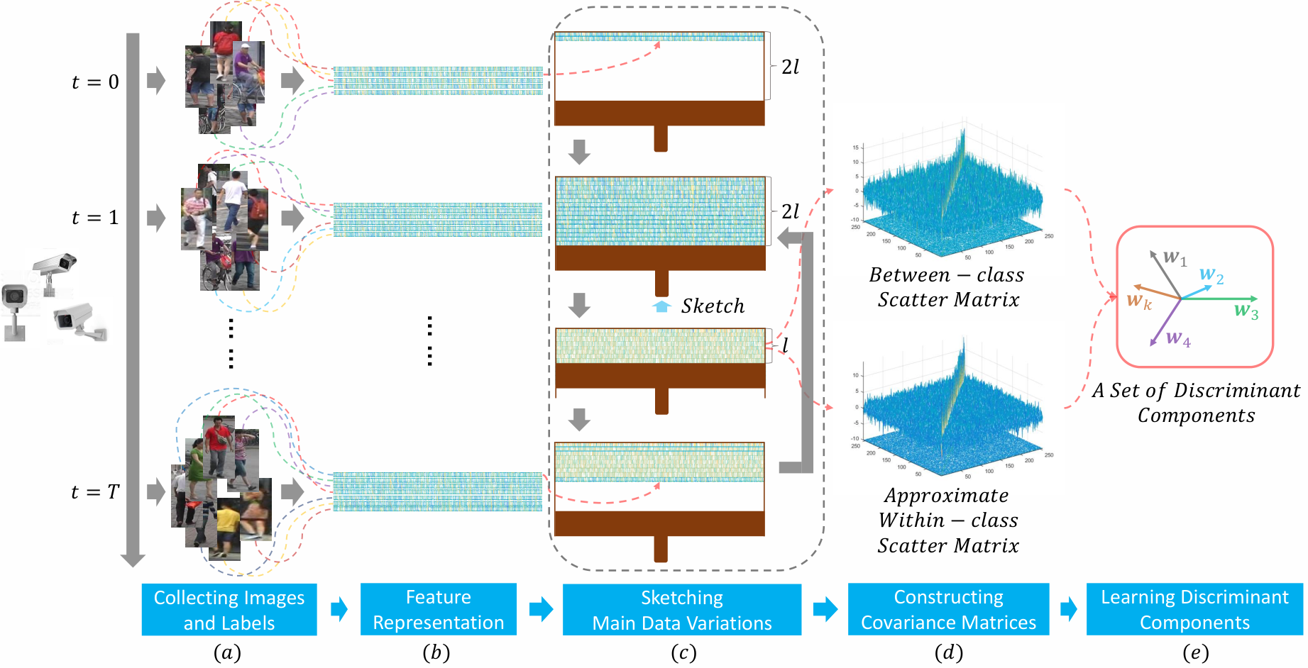
In this section, we start to present the Sketch online Discriminant Analysis (SoDA) for Person re-identification. In real-world scenario, samples come endlessly and sequentially from vision system (Figure 1). The number of samples received in each round is random, and the individual sample obtained is also stochastic. Suppose the new coming sample represented as a dimensional feature vector is labelled with class label . For convenience, at the round, we denote all passed data (i.e. training samples collected in the current and previous rounds) as a training sample matrix , and denote all the corresponding labels as where is the class label of and .
At each round (), the proposed SoDA maintains the main variations of all passed data () in a low rank matrix, which is named as the “sketch matrix”. The sketch matrix keeps a small number of selected frequent directions, which are obtained and updated by a matrix sketch technique during the whole online learning process. While sketching main data variations, the population mean and the one of each class are also updated. We further utilize these updated means and the low rank sketch matrix to estimate between-class covariance matrix and derive the approximate within-class covariance matrix after all new coming samples are compressed into the sketch matrix. Finally, we generate discriminant components by eigenvalue decomposition for simultaneously minimizing the approximate within-class variance and maximizing the between-class variance. The whole procedure of SoDA is illustrated in Figure 1 and presented in Algorithm 1. The in-depth theoretical investigation to explain why SoDA can approximate the offline FDA model by sketch and guarantee its effectiveness on extracting discriminant components is provided in Sec. IV.
III-A Estimating Between-class covariance matrix
During online learning, we keep updating the population mean and mean of each class ( = 1, 2, , ) so as to construct the between-class covariance matrix . When having a new coming sample with class label , the population mean and mean of class are updated by
| (1) |
and the population number and the number of samples for class are also updated by:
| (2) |
We then use the updated means to estimate the between-class covariance matrix as follows:
| (3) |
III-B Estimating Approximate Within-class covariance matrix
For realizing one-pass online learning, we aim to update/form the within-class covariance matrix which describes the within-class variation without using any passed observed data samples. Different from previous online FDA approaches, we embed sketch processing into FDA and derive a novel approximate within-class covariance matrix efficiently and effectively. For this purpose, we first employ the sketch technique [24] to compress the passed data samples into a sketch matrix so as to maintain the main variations of passed data. More specifically, we maintain the main variations of all passed data in a small size matrix , called a sketch matrix, where is initialized by a zero matrix. Each new coming sample (i.e. the -th row of ) replaces a zero row of from top to bottom until is full without any all zero rows. When is full, we apply Singular Value Decomposition (SVD) on such that , where is a diagonal matrix with singular values on the diagonal in decreasing order. Each row in corresponds to a singular value in , and let vectors of corresponding to the first half singular values denoted as and the ones corresponding to lower half singular values denoted as . By employing the sketch algorithm, the frequent directions are scaled by and retained in , where is the largeast singular value in of . In this way, the sketch matrix is obtained by , where and is a zero matrix. Therefore, the sketch matrix is a matrix, where , the upper half of , retains the main variations of passed data samples, and , the lower half of , is reset to zero.
Although no passed observed data samples are saved, we propose to derive an approximate within-class covariance matrix using the sketch matrix below:
| (4) |
where
| (5) |
In the above, is not always the exact within-class covariance matrix but it is an approximate one. In Sec. IV, we will provide in-depth theoretical analysis of the bias of this approximation on discriminant feature component extraction.
III-C Dimension Reduction and Extraction of Discriminant Components
Normally, after updating the two covariance matrices and , it is only necessary to compute the generalized eigen-vectors of . However, in person re-identification, some kinds of features are of high dimensionality such as HIPHOP [5], LOMO [22] and etc, and the size of the two covariance matrices and was determined by the feature dimensionality. Thus the above eigen-decomposition remains costly when the size of both and are large.
An intuitive solution is to conduct another online learning for dimension reduction, which spends extra time and space. However, SoDA does not require such an extra learning. Due to sketch, SoDA actually maintains a set of frequent directions that describe main data variations. And thus we take these frequent directions as basis vectors and the span of them can approximate the data space. Hence, we set , the upper half of matrix (Line 16 in Algorithm 1), and the dimension reduction is performed by:
| (6) |
where consists of frequent directions. In this way, and become matrices in , and computing generalized eigen-vectors will become much faster. Finally, the generalized eigen-vectors (Line 22 in Algorithm 1) are computed by , and they are the discriminant components we pursuit.
III-D Computational Complexity
As presented above, after processing all observed samples, we maintain , , and ( = 0, 1, 2, …, ). The time and space cost of the rest procedure is (After the whole processing, is equal to ) and , respectively. Therefore, the cost of time and space is and , respectively, almost the same as the cost of sketch algorithm [24].
IV Theoretical Analysis
In this section, we theoretically show that SoDA approximates FDA in a principled way, although SoDA is formed based on the approximate within-class covariance matrix mined from sketch data information.
IV-A Fisher Discriminant Analysis
Fisher discriminant analysis (FDA) aims to seek discriminant projections for minimizing within-class variance and maximizing between-class variance, which are estimated over the data matrix and its label set in an offline way. There are several equivalent criteria for the multi-class case. For analysis, we consider the one that maxmizes the following criterion:
| (7) |
where is the between-class covariance matrix and is the within-class covariance matrix. They are given by
| (8) |
| (9) |
where and are the data mean and the number of samples of the class, respectively, and and are the population number and population mean, respectively. And the total covariance matrix is
| (10) |
Generally, the analysis seeks a set of feature vectors that maximize the criterion subject to the normalization constraint , where is the matrix whose columns are . This leads to the computation of generalized eigenvectors, that is and is a diagonal matrix with generalized eigenvalues on the diagonal. Here, the eigenvectors corresponding to the largest eigenvalues are used to compress a high dimensional data vector to a low dimensional feature representation.
IV-B Relation between SoDA and FDA
Before presenting the theoretical analysis, we first define the following notations. Let
| (11) |
where is the conventional FDA criterion and is SoDA criterion by replacing with that is mined from sketch data information.
Let the largest Fisher scores in the above equations be
| (12) |
Since for optimizing Eqs. (12), we can form a Lagrangian function by imposing the constraint for both criteria [41] We define , and thus we can reform Eqs. (12) by:
| (13) |

In the following sections, we first discuss the relationship between and . And then this relationship will be used to present a bound for . Note that is to measure how well the optimal projection learned by our SoDA approximates the optimal solution that maximizes . Note that our analysis will not take any dimension reduction before extracting discriminant components below for discussion. Our analysis can be extended if the same dimension reduction is applied to all methods discussed below.
IV-C Relationship Between the Maximum Fisher Score of FDA and that of SoDA
We first present the relationship between the maximum Fisher score of FDA and the one of SoDA, i.e. the relationship between and . Suppose that matrix is the totally training sample set consisting of samples acquired at each time step.
However, it is not intuitive to obtain the relationship between the maximum Fisher score of FDA and the one of SoDA based on the covariance matrices inferred in Eq. (5). In order to exploit such a relationship, we first investigate the Fisher score obtained by and the approximate within-class covariance matrix as follows:
| (14) |
Let be the within-class covariance matrix computed in batch mode (i.e. for offline FDA). Since it is known that , it can be verified that
| (15) |
By combining Eq. (25) as stated in the Appendix, it is not hard to have the following theorem about the relation between and , and we visualize the approximation between the groundtruth within-class covaraince matrix and our approximate one in Figure 2. We assume that , and are not singular in the following analysis 11 1 The analysis can be generalized to the case when is not invertible if the same regularization is imposed on both , and .
Theorem 1.
and , where is the induced norm of a matrix and is the Frobenius norm.
Based on the above theorem, we particularly consider the two-class classification case.
Theorem 2.
Considering the two criteria in Eq. (13) when the discriminant feature transformation is a one-dimensional vector, i.e. and , the relationship between and is as follow:
| (16) |
where is the smallest (non-zero) singular value of matrix and .
Proof.
Let . From the Theorem 1, we have . That is
| (17) |
From the theorem above, we can claim that the largest Fisher score is always greater than or equal to the original one after sketch. From another aspect, the inequalities “” means when more rows are set in the sketch matrix , (i.e. much larger is set), becomes , and thus SoDA becomes exactly the FDA.
For the multi-class case, we can generalize the above proof below.
Theorem 3.
Considering the two criteria in Eq. (13), when the discriminant feature transformation is a -dimensional transformation where , we have .
Proof.
| Approaches | IFDA [15] | Pang’s IFDA [33] | IDR/QR [48] | OL-IDM [37] | Wang et al. [39] | Martinel et al. [29] | SoDA (Ours) |
| Save within-class | ✓ | ✓ | ✓ | - - | - - | - - | ✗ |
| scatter matrix? | |||||||
| Save between-class | ✓ | ✓ | ✗ | - - | - - | - - | ✗ |
| scatter matrix? | |||||||
| Is an one-pass | ✗ | ✓ | ✓ | ✓ | ✗ | ✗ | ✓ |
| algorithm? | |||||||
| Human feedback | ✗ | ✗ | ✗ | ✗ | ✓ | ✓ | ✗ |
| Can the model be | ✓ | ✓ | ✓ | ✓ | ✗ | ✗ | ✓ |
| trained on streaming data? | |||||||
| Is the model embedded | ✗ | ✗ | ✗ | ✗ | ✗ | ✗ | ✓ |
| with dimension reduction? | |||||||
| time | - - | - - | - - | ||||
| complexity | |||||||
| space | - - | - - | - - | ||||
| complexity |
IV-D How Does the Projection Learned by SoDA Optimize the Original Fisher Criterion Approximately?
In the above, we analyze the quotient values between and . However, in SoDA, our within-class covariance matrix is estimated by sketch and is not the exact within-class covariance matrix. In the following, we will present the effect of the learned discriminant component using SoDA on minimizing the grouth-truth within-class covariance. For this purpose, the following theorems are presented.
Theorem 4.
For any , we have
| (19) |
Proof.
Theorem 5.
Considering the two criteria in Eq. (13), we define , denote the smallest non-zero singular value of as , and let . Suppose the norm of each data vector (i.e. each row of the data matrix ) is bounded by , that is Then we have
| (20) |
Proof.
First, given
| (21) |
Since , we have . Here, for convenience, one can further assume , otherwise a much tighter bound can be inferred. And thus . So we have
| (22) |
Note that since it is assumed that . Thus, under the constraint , we have
| (23) |
where the latter equation is obvious since may not be the optimal projection for mamixizing . Finally, since and that means the norm of any data vector (i.e. each row of the data matrix ) is bounded by , we have
| (24) |
∎

IV-E Discussion
IV-E1 SoDA vs. FDA
The above theorem indicates that 1) the learned transformation by SoDA may not be the optimal one for the FDA directly learned on all observed data since , which is obvious and reasonable; 2) however, there is a lower bound on , since ; 3) as long as more and more rows are set in the sketch matrix used in SoDA, i.e. is larger and larger, and so that in such a case. The latter case is reasonable because although the sketch in SoDA enables selecting data variation during the online learning, more data information is kept when a much larger sketch matrix is used, and this will be verified in the experiments (see Figure 3 for example).
IV-E2 SoDA vs. Incremental/online models
In Table I, we compare SoDA with related incremental/online FDA models in details. A distinct and important characteristic of SoDA is that it is able to perform one-pass online learning directly only relying on sketch data information. SoDA does not have to keep within-class covariance matrix and between-class covariance matrix in memory during online learning, due to embedding sketch processing, which has not been considered for online learning of FDA before. Moreover, as compared to the others, SoDA does not need any extra online learning progress on dimension reduction, which is naturally embedded. Thus the training cost of SoDA is much lighter.
When applied SoDA to person re-id, we perform the comparison with related online person re-id models. An important distinction is that no extra human feedback is required, and SoDA is able to be applied on streaming data in an one-pass learning manner. In comparison with OL-IDM, SoDA has its merits: 1) dimension reduction is naturally embedded in SoDA; 2) embedding sketch into person re-id model learning is a more efficient and effective way to maintain the main variations of data, which has been verified by our experimental results.
V Experiments
V-A Datasets and Evaluation Settings
V-A1 Datasets
We extensively evaluated the proposed approach on three large person re-id benchmarks: Market-1501, SYSU, and ExMarket.
- •
Market-1501 dataset [51] contains person images collected in front of a campus supermarket at a University. It consists of 32,643 person images of 1,501 identities.
- •
SYSU dataset contains totally 48,892 images of 502 pedestrians captured by two cameras. Similar to [4], we randomly selected 251 identities from two views as training set which contains 12308 images. And we randomly selected three images of each person from the rest 251 identities of both cameras to form the testing set, where the 753 images of the first camera were used as query images.
- •
ExMarket dataset was formed by combining the MARS dataset [50] and Market-1501 dataset. MARS was formed as a video dataset for person re-identification. All the identities from MARS are of a subset of those from Market. More specifically, for each identity, we extracted one frame for each five consecutive frames firstly and combined images extracted from MARS and the ones from Market-1501 of the same person. Therefore, ExMarket contains 237147 images of 1501 identities, the largest population size among the three benchmark datasets tested.
V-A2 Features
In this work, we conducted the evaluation based on four types of feature for evaluation: 1) JSTL, 2) LOMO, 3) HIPHOP, 4) JSTL + LOMO + HIPHOP (JLH).
- •
JSTL is a kind of low-dimensional deep feature representation () extracted by a deep convolutional network [43];
- •
LOMO is an effective handcraft feature proposed for person re-id in [22], and it is a 26960-dimensional vector;
- •
HIPHOP is another recently proposed person re-id feature () [5] that extracts more view invariant histogram features from shallow layers of a convolution network.
In addition, since person re-id can benefit from using multiple different types of appearance features as shown in [5, 7, 9, 49, 52]. we concatenated JSTL, LOMO and HIPHOP as a high dimensional feature (), named JLH in this work for convenience of description. On all datasets, we report experimental results of SoDA using the concatenated feature in Table VI. Since LOMO, HIPHOP, and JLH are of high dimension, for all methods except SoDA, we first reduced their feature dimension of the three types of feature to 2000, 2000 and 2500, respectively, on all datasets. For SoDA, we set the sketch size () to the (reduced) feature dimension menthioned above on all datasets.
V-A3 Evaluation protocol
On all datasets, we followed the standard evaluation settings on person re-identification, i.e. images of half of the persons were used for training and images of the rest half were used for testing, so that there is no overlap in persons between training and testing sets. More specifically, on Market-1501 dataset, we used the standard training (12936 images of 750 people) and testing (19732 images of 751 people) sets provided in [51]. On SYSU dataset, similar to [4], we randomly picked all images of the selected 251 identities from two views to form the training set which contains 12308 images, and we randomly picked 3 images of each pedestrian of the rest 251 identities in each view for forming the gallery and query sets for testing. On ExMarket dataset, we conducted the same identity split as the Market-1501 dataset. The training set contains 112351 images, and the testing set contains 124796 images, among which 3363 images are considered as query images and the rest are considered as gallery images.
| Feature | JSTL | LOMO | HIPHOP | JLH | |||||||||||||||||
| Dataset | Method | rank-1 | rank-5 | rank-10 | rank-20 | mAP | rank-1 | rank-5 | rank-10 | rank-20 | mAP | rank-1 | rank-5 | rank-10 | rank-20 | mAP | rank-1 | rank-5 | rank-10 | rank-20 | mAP |
| Market | FDA | 57.30 | 75.53 | 81.38 | 86.49 | 28.57 | 51.90 | 74.26 | 81.12 | 87.14 | 23.60 | 60.27 | 80.52 | 87.05 | 91.18 | 31.45 | 74.20 | 88.75 | 92.19 | 94.80 | 49.01 |
| -1501 | SoDA | 57.13 | 74.79 | 81.18 | 85.90 | 28.25 | 52.41 | 73.37 | 81.38 | 87.17 | 23.58 | 61.88 | 81.41 | 86.70 | 91.60 | 33.39 | 75.27 | 89.28 | 92.70 | 95.22 | 49.82 |
| SYSU | FDA | 31.21 | 52.99 | 61.49 | 71.85 | 25.86 | 46.61 | 70.78 | 79.42 | 86.19 | 41.81 | 52.86 | 73.84 | 81.67 | 87.78 | 48.20 | 63.08 | 80.35 | 86.32 | 91.50 | 56.82 |
| SoDA | 31.74 | 52.86 | 62.15 | 71.31 | 26.04 | 47.81 | 70.39 | 78.75 | 86.72 | 41.69 | 53.12 | 73.97 | 80.88 | 87.25 | 48.48 | 64.81 | 80.74 | 87.25 | 91.77 | 59.82 | |
| Ex- | FDA | 53.89 | 68.11 | 73.13 | 77.97 | 22.71 | 45.64 | 60.42 | 66.86 | 72.89 | 17.98 | 57.24 | 71.38 | 77.11 | 81.74 | 27.20 | 66.86 | 78.18 | 82.63 | 86.70 | 39.00 |
| Market | SoDA | 54.93 | 68.79 | 73.13 | 77.46 | 22.87 | 46.08 | 61.31 | 67.81 | 73.63 | 17.77 | 55.76 | 70.40 | 76.10 | 81.59 | 24.97 | 66.18 | 78.36 | 82.48 | 86.64 | 37.11 |
| Dataset | Market-1501 | SYSU | ExMarket | ||||||
|---|---|---|---|---|---|---|---|---|---|
| Method | rank-1 | mAP (%) | Accumulative | rank-1 | mAP (%) | Accumulative | rank-1 | mAP (%) | Accumulative |
| matching rate (%) | Time (s) | matching rate (%) | Time (s) | matching rate (%) | Time (s) | ||||
| OL-IDM | 31.50 | 10.48 | 3706.84 | 12.08 | 10.29 | 10588.15 | 50.24 | 18.93 | 1646433.70 |
| IDR/QR | 41.15 | 13.20 | 803.59 | 12.88 | 10.24 | 247.17 | 42.70 | 11.20 | 6172.79 |
| IFDA | 51.45 | 21.21 | 38.22 | 22.97 | 18.12 | 12.40 | 49.91 | 16.58 | 394.31 |
| Pang’s IFDA | 57.36 | 28.58 | 13.68 | 31.08 | 25.28 | 7.65 | 55.46 | 22.97 | 120.94 |
| SoDA | 57.13 | 28.25 | 7.84 | 31.74 | 26.04 | 4.68 | 54.93 | 22.87 | 50.52 |
| Dataset | Market-1501 | SYSU | ExMarket | ||||||
|---|---|---|---|---|---|---|---|---|---|
| Method | rank-1 | mAP (%) | Accumulative | rank-1 | mAP (%) | Accumulative | rank-1 | mAP (%) | Accumulative |
| matching rate (%) | Time (s) | matching rate (%) | Time (s) | matching rate (%) | Time (min) | ||||
| OL-IDM | 3.95 | 0.73 | 736707.11 | 1.06 | 1.59 | 743335.02 | 3.86 | 0.33 | 1 week |
| IDR/QR | 19.36 | 5.09 | 345181.63 | 6.37 | 5.16 | 83903.98 | 19.92 | 3.58 | 74393.24 |
| IFDA | 38.75 | 13.32 | 314470.08 | 26.83 | 22.59 | 67003.60 | 35.63 | 10.43 | 69668.26 |
| Pang’s IFDA | 44.80 | 18.64 | 314461.09 | 35.99 | 31.82 | 66646.88 | 43.50 | 15.42 | 69625.84 |
| SoDA | 52.41 | 23.53 | 2127.47 | 47.81 | 41.69 | 3345.30 | 46.08 | 17.77 | 359.28 |
| Dataset | Market-1501 | SYSU | ExMarket | ||||||
|---|---|---|---|---|---|---|---|---|---|
| Method | rank-1 | mAP (%) | Accumulative | rank-1 | mAP (%) | Accumulative | rank-1 | mAP (%) | Accumulative |
| matching rate (%) | Time (s) | matching rate (%) | Time (s) | matching rate (%) | Time (s) | ||||
| OL-IDM | 11.97 | 2.22 | 277104.72 | 1.46 | 2.00 | 252626.33 | 7.24 | 0.54 | 1 week |
| IDR/QR | 19.98 | 6.00 | 225226.32 | 10.49 | 9.34 | 86513.64 | 21.97 | 5.32 | 2392922.71 |
| IFDA | 52.14 | 21.30 | 185390.31 | 25.50 | 22.32 | 66202.88 | 46.08 | 15.50 | 2133499.12 |
| Pang’s IFDA | 60.42 | 31.30 | 185174.97 | 51.79 | 47.51 | 65593.56 | 54.84 | 25.11 | 2135671.23 |
| SoDA | 61.88 | 33.39 | 3620.00 | 53.12 | 48.48 | 13849.61 | 55.76 | 24.97 | 83319.79 |
On all datasets, the cumulative matching characteristic (CMC) curves is shown to measure the performance of the compared methods on re-identifying individuals across different camera views under online setting. In addition to this, we also report results using another two performance metrics: 1) rank-1 Matching Rate, and 2) mean Average Precision (mAP). mAP first computes the area under the Precision-Recall curve for each query and then calculates the mean of Average Precision over all query persons. All experiments were implemented using MATLAB on a machine with CPU E5 2686 2.3 GHz and 256 GB RAM, and the accumulative time of all compared methods were also computed and reported for measuring efficiency.
V-B SoDA vs. FDA
In Sec. IV, we provide theoretical analysis on the relation between SoDA and FDA. In this section, we provide empirical evaluation on three datasets by the comparison on Fisher Score between SoDA and FDA in Figure 3. The figure indicates that by keeping more rows in the sketch matrix, SoDA can acquire more similar Fisher Score as the one of FDA, and this is supported by Theorem 5. We also compared SoDA with FDA on the three datasets in Table II, and the comparison shows that they work comparably. Therefore the results reported here have validated that our sketch approach approximates FDA (i.e. the offline model) for extracting discriminant information very well, and thus the effectiveness of our model is verfied both theoretically and empirically.
V-C SoDA vs. Incremental FDA Model
| Dataset | Market-1501 | SYSU | ExMarket | ||||||
|---|---|---|---|---|---|---|---|---|---|
| Method | rank-1 | mAP (%) | Accumulative | rank-1 | mAP (%) | Accumulative | rank-1 | mAP (%) | Accumulative |
| matching rate (%) | Time (s) | matching rate (%) | Time (s) | matching rate (%) | Time (s) | ||||
| OL-IDM | 14.43 | 2.48 | 356136.53 | 3.32 | 4.91 | 554908.70 | 10.84 | 0.70 | 1 week |
| IDR/QR | 36.70 | 13.73 | 251934.68 | 15.80 | 12.82 | 220962.28 | 39.64 | 10.85 | 2479401.99 |
| IFDA | 61.19 | 30.36 | 203537.09 | 21.65 | 18.23 | 189960.96 | 56.24 | 23.46 | 2032679.17 |
| Pang’s IFDA | 71.64 | 45.15 | 204406.03 | 56.31 | 49.60 | 189897.24 | 64.64 | 34.80 | 2036601.02 |
| SoDA | 75.27 | 49.82 | 12952.07 | 64.81 | 59.82 | 9951.20 | 66.18 | 37.11 | 164475.67 |
| Method | rank-1 | rank-5 | rank-10 | rank-20 | Map |
| CRAFT | 71.20 | 87.35 | 391.69 | 94.39 | 44.24 |
| MLAPG | 69.33 | 85.63 | 90.23 | 93.82 | 46.16 |
| KISSME | 67.99 | 83.67 | 88.93 | 92.79 | 39.79 |
| XQDA | 67.96 | 83.91 | 88.95 | 93.14 | 43.89 |
| SoDA | 75.27 | 89.28 | 92.70 | 95.22 | 49.82 |
| Method | rank-1 | rank-5 | rank-10 | rank-20 | mAP |
| CRAFT | 24.70 | 43.03 | 55.11 | 67.73 | 23.31 |
| MLAPG | 18.46 | 35.86 | 47.01 | 58.83 | 18.03 |
| KISSME | 62.28 | 79.81 | 86.06 | 90.31 | 56.23 |
| XQDA | 64.14 | 80.88 | 86.85 | 91.90 | 59.12 |
| SoDA | 64.81 | 80.74 | 87.25 | 91.77 | 59.82 |
| Method | rank-1 | rank-5 | rank-10 | rank-20 | mAP |
| CRAFT | 54.51 | 69.39 | 75.56 | 80.94 | 24.26 |
| MLAPG | 50.21 | 65.29 | 70.90 | 77.20 | 25.63 |
| KISSME | 57.42 | 69.71 | 74.23 | 78.83 | 30.03 |
| XQDA | 55.05 | 68.02 | 73.10 | 77.73 | 28.36 |
| SoDA | 66.18 | 78.36 | 82.48 | 86.64 | 37.11 |
There are existing works that are related to incremental learning of FDA, which also process sequential data and update the models online. We compared extensively our method SoDA with three related online/incremental FDA methods, including IFDA [15], IDR/QR [48] and Pang’s IFDA [33]. We show CMC curve of all methods using different types of features in Figure 4, Figure 6, Figure 7 and Figure 8. The results illustrate that the proposed SoDA outperformed the compared incremental FDA. For instance, when using JLH, SoDA outperformed Pang’s IFDA and achieved 75.27%, 64.81% and 66.18% rank-1 matching rate on Market, SYSU and ExMarket, respectively. We further report mAP and accumulative time in Table III, Table IV, Table V and Table VI. It suggests that SoDA has a better mAP values especially on SYSU and spends much less time, where for instance SoDA gains around 60% reduction on the cost of computation time, as compared with Pang’s ILDA.
V-D SoDA vs. Related Person re-id Models
Comparison with online re-id model. We compared the online re-id method OL-IDM [37] that addresses the same setting as ours in this work. Table III, IV, V and VI tabulate the comparison results. It is noteworthy that our SoDA obtains much more stable results on rank-1 matching rate and mAP performance. Moreover, SoDA is more efficient than OL-IDM, taking 30 times smaller accumulative time.
Comparison with related subspace model and classical models. We also compared two related subspace model for person re-identification: 1) CRAFT [5] ; 2) MLAPG [23], and two classical methods: 1) KISSME [16] ; 2) XQDA [22], when the JLH feature was applied on all datasets. All of these methods were learned in an offline way, and the results of these methods on all benchmarks using JLH features are presented in Table VII, VIII and IX. Among all compared methods, the rank-1 matching rate and mAP of SoDA are the highest, and its accumulative time is the lowest. This indicates that SoDA achieves better or comparable performance of the related off-line subspace person re-id models.
V-E Further Evaluation of SoDA
Effect of the sketch size using low dimensional feature. On all benchmarks, we conducted experiments using JSTL feature (dimensional) for evaluating the effect of the sketch size on low dimensional feature. The experimental results in Figure 10 indicate that the performance of our proposed SoDA can be improved when (i.e. the rank of ) is larger. That is the performance is better when more variations of passed data are remained in the sketch matrix. It is reasonable because when more data variations are reserved, the estimated within-class covariance matrix from the sketch matrix can approximate the ground-truth one better. However, larger indeed increases the accumulative time since the computation complexity and memory depend on when the number of samples and the dimensionality of features are determined (Sec. III-D). Fortunately, we empirically find that good performance and low accumulative time can be achieved at the same time when setting the rank of the sketch matrix to a properly small value, i.e. .
Effect of the sketch size using high dimensional features. We also show the effect of when using high dimensional features, as some recent proposed state-of-the-art person re-id features are of high dimension, such as LOMO (dimensional), HIPHOP (dimensional) and also the JLH (dimensional) formed in this work. High dimensionality will increase the computational and space complexities (e.g., the whole training data matrix of ExMarket is a matrix). Instead of conducting another online learning for dimension reduction, SoDA utilizes a set of orthogonal frequent directions maintained by the sketch matrix for reducing feature dimension. The experimental results shown in Figure 10 and Figure 9 again verify that increasing the sketch size can improve the performance of SoDA but also increase the accumulative time due to extra computation for dimension reduction. Also, on high dimensional feature, setting to be a properly small value (e.g. ) can gain a good balance between good performance and low accumulative computation time.
VI Conclusion
We contribute to developing a succinct and effective online person re-identification (re-id) methods namely SoDA. Compared with existing online person re-id models, SoDA performs one-pass online learning without any explicit storage of passed observed data samples, meanwhile preserving a small sketch matrix that describes the main variation of passed observed data samples. And moreover, SoDA is able to be trained on streaming data efficiently with low computational cost, upon on no elaborated human feedback. Compared with the related online FDA models, we take a novel approach by embedding sketch processing into FDA, and we approximately estimate the within-class variation from a sketch matrix and finally derive SoDA for extracting discriminant components. More importantly, we have provided in-depth theoretical analysis on how the sketch information affects the discriminant component analysis. The rigorous upper and lower bounds on how SoDA approaches its offline model (i.e. the classical Fisher Discriminant Analysis) are given and proved. Extensive experimental results have clearly illustrated the effectiveness of our SoDA and verified our theoretical analysis.
Acknowledgement
This research was supported by the NSFC (No. 61472456, No. 61573387, No. 61522115).
References
- [1] E. Ahmed, M. Jones, and T. K. Marks. An improved deep learning architecture for person re-identification. In CVPR, 2015.
- [2] G. Chechik, V. Sharma, U. Shalit, and S. Bengio. Large scale online learning of image similarity through ranking. JMLR, 11(Mar):1109–1135, 2010.
- [3] Y.-C. Chen, W.-S. Zheng, and J. Lai. Mirror representation for modeling view-specific transform in person re-identification. In IJCAI, 2015.
- [4] Y.-C. Chen, W.-S. Zheng, J.-H. Lai, and P. Yuen. An asymmetric distance model for cross-view feature mapping in person re-identification. TCSVT, 2016.
- [5] Y.-C. Chen, X. Zhu, W.-S. Zheng, and J.-H. Lai. Person re-identification by camera correlation aware feature augmentation. TPAMI, 2017.
- [6] K. Crammer, O. Dekel, J. Keshet, S. Shalev-Shwartz, and Y. Singer. Online passive-aggressive algorithms. JMLR, 7(Mar):551–585, 2006.
- [7] M. Farenzena, L. Bazzani, A. Perina, V. Murino, and M. Cristani. Person re-identification by symmetry-driven accumulation of local features. In CVPR, 2010.
- [8] S. Furao and O. Hasegawa. An incremental network for on-line unsupervised classification and topology learning. NN, 19(1):90–106, 2006.
- [9] D. Gray and H. Tao. Viewpoint invariant pedestrian recognition with an ensemble of localized features. In ECCV, 2008.
- [10] K. Hiraoka, K.-i. Hidai, M. Hamahira, H. Mizoguchi, T. Mishima, and S. Yoshizawa. Successive learning of linear discriminant analysis: Sanger-type algorithm. In ICPR, 2000.
- [11] L.-K. Huang, Q. Yang, and W.-S. Zheng. Online hashing. TNNLS, 2017.
- [12] P. Jain, B. Kulis, I. S. Dhillon, and K. Grauman. Online metric learning and fast similarity search. In ANIPS, 2009.
- [13] X.-Y. Jing, X. Zhu, F. Wu, X. You, Q. Liu, D. Yue, R. Hu, and B. Xu. Super-resolution person re-identification with semi-coupled low-rank discriminant dictionary learning. In CVPR, 2015.
- [14] T.-K. Kim, J. Kittler, and R. Cipolla. On-line learning of mutually orthogonal subspaces for face recognition by image sets. TIP, 19(4):1067–1074, 2010.
- [15] T.-K. Kim, B. Stenger, J. Kittler, and R. Cipolla. Incremental linear discriminant analysis using sufficient spanning sets and its applications. IJCV, 91(2):216–232, 2011.
- [16] M. Koestinger, M. Hirzer, P. Wohlhart, P. M. Roth, and H. Bischof. Large scale metric learning from equivalence constraints. In CVPR, 2012.
- [17] M. Koestinger, M. Hirzer, P. Wohlhart, P. M. Roth, and H. Bischof. Large scale metric learning from equivalence constraints. In CVPR, 2012.
- [18] H. Li, Y. Li, and F. Porikli. Deeptrack: Learning discriminative feature representations online for robust visual tracking. TIP, 25(4):1834–1848, 2016.
- [19] X. Li, C. Shen, A. Dick, Z. M. Zhang, and Y. Zhuang. Online metric-weighted linear representations for robust visual tracking. TPAMI, 38(5):931–950, 2016.
- [20] X. Li, W.-S. Zheng, X. Wang, T. Xiang, and S. Gong. Multi-scale learning for low-resolution person re-identification. In ICCV, 2015.
- [21] J. Liang, Q. Hu, W. Wang, and Y. Han. Semisupervised online multikernel similarity learning for image retrieval. TMM, 19(5):1077–1089, 2017.
- [22] S. Liao, Y. Hu, X. Zhu, and S. Z. Li. Person re-identification by local maximal occurrence representation and metric learning. In CVPR, 2015.
- [23] S. Liao and S. Z. Li. Efficient psd constrained asymmetric metric learning for person re-identification. In ICCV, 2015.
- [24] E. Liberty. Simple and deterministic matrix sketching. In SIGKDD, KDD ’13, 2013.
- [25] C. Liu, C. Change Loy, S. Gong, and G. Wang. Pop: Person re-identification post-rank optimisation. In ICCV, 2013.
- [26] G.-F. Lu, J. Zou, and Y. Wang. Incremental complete lda for face recognition. PR, 45(7):2510–2521, 2012.
- [27] L. Ma, X. Yang, and D. Tao. Person re-identification over camera networks using multi-task distance metric learning. TIP, 23(8):3656–3670, 2014.
- [28] N. Martinel, A. Das, C. Micheloni, and A. K. Roy-Chowdhury. Re-identification in the function space of feature warps. TPAMI, 37(8):1656–1669, 2015.
- [29] N. Martinel, A. Das, C. Micheloni, and A. K. Roy-Chowdhury. Temporal model adaptation for person re-identification. In ECCV, 2016.
- [30] A. Mignon and F. Jurie. Pcca: A new approach for distance learning from sparse pairwise constraints. In CVPR, 2012.
- [31] S. Paisitkriangkrai, C. Shen, and A. van den Hengel. Learning to rank in person re-identification with metric ensembles. In CVPR, 2015.
- [32] R. Panda, A. Bhuiyan, V. Murino, and A. K. Roy-Chowdhury. Unsupervised adaptive re-identification in open world dynamic camera networks. In CVPR, 2017.
- [33] S. Pang, S. Ozawa, and N. Kasabov. Incremental linear discriminant analysis for classification of data streams. TSMCB, 35(5):905–914, 2005.
- [34] Y. Peng, S. Pang, G. Chen, A. Sarrafzadeh, T. Ban, and D. Inoue. Chunk incremental idr/qr lda learning. In IJCNN, 2013.
- [35] B. Prosser, W.-S. Zheng, S. Gong, T. Xiang, and Q. Mary. Person re-identification by support vector ranking. In BMCV, 2010.
- [36] F. Schroff, D. Kalenichenko, and J. Philbin. Facenet: A unified embedding for face recognition and clustering. In CVPR, 2015.
- [37] Y. Sun, H. Liu, and Q. Sun. Online learning on incremental distance metric for person re-identification. In RB, 2014.
- [38] M. Uray, D. Skocaj, P. M. Roth, H. Bischof, and A. Leonardis. Incremental lda learning by combining reconstructive and discriminative approaches. In BMVC, 2007.
- [39] H. Wang, S. Gong, X. Zhu, and T. Xiang. Human-in-the-loop person re-identification. In ECCV, 2016.
- [40] M. K. Warmuth and D. Kuzmin. Randomized online pca algorithms with regret bounds that are logarithmic in the dimension. JMLR, 9(Oct):2287–2320, 2008.
- [41] A. R. Webb. Statistical pattern recognition. 2003.
- [42] P. Wu, S. C. Hoi, P. Zhao, C. Miao, and Z.-Y. Liu. Online multi-modal distance metric learning with application to image retrieval. TKDE, 28(2):454–467, 2016.
- [43] T. Xiao, H. Li, W. Ouyang, and X. Wang. Learning deep feature representations with domain guided dropout for person re-identification. In CVPR, 2016.
- [44] F. Xiong, M. Gou, O. Camps, and M. Sznaier. Person re-identification using kernel-based metric learning methods. In ECCV, 2014.
- [45] J. Yan, B. Zhang, S. Yan, Q. Yang, H. Li, Z. Chen, W. Xi, W. Fan, W.-Y. Ma, and Q. Cheng. Immc: incremental maximum margin criterion. In SIGKDD, 2004.
- [46] J. Yang, A. F. Frangi, J.-y. Yang, D. Zhang, and Z. Jin. Kpca plus lda: a complete kernel fisher discriminant framework for feature extraction and recognition. TPAMI, 27(2):230–244, 2005.
- [47] H. Yao, S. Zhang, D. Zhang, Y. Zhang, J. Li, Y. Wang, and Q. Tian. Large-scale person re-identification as retrieval.
- [48] J. Ye, Q. Li, H. Xiong, H. Park, R. Janardan, and V. Kumar. Idr/qr: an incremental dimension reduction algorithm via qr decomposition. TKDE, 17(9):1208–1222, 2005.
- [49] L. Zhang, T. Xiang, and S. Gong. Learning a discriminative null space for person re-identification. In CVPR, 2016.
- [50] L. Zheng, Z. Bie, Y. Sun, J. Wang, C. Su, S. Wang, and Q. Tian. Mars: A video benchmark for large-scale person re-identification. In ECCV, pages 868–884. Springer, 2016.
- [51] L. Zheng, L. Shen, L. Tian, S. Wang, J. Wang, and Q. Tian. Scalable person re-identification: A benchmark. In ICCV, 2015.
- [52] L. Zheng, S. Wang, L. Tian, F. He, Z. Liu, and Q. Tian. Query-adaptive late fusion for image search and person re-identification. In CVPR, 2015.
- [53] W.-S. Zheng, S. Gong, and T. Xiang. Person re-identification by probabilistic relative distance comparison. In CVPR, 2011.
- [54] W.-S. Zheng, X. Li, T. Xiang, S. Liao, J. Lai, and S. Gong. Partial person re-identification. In ICCV, 2015.
Matrix Sketch. The sketch technique we discuss in this work is related to the matrix sketch [24], which is pass-efficient to read streaming data at most a constant number of time. The sketch algorithm learns a set of frequent directions from an matrix in a stream, where each row of is a -dimensional vector. It maintains a sketch matrix containing rows and guarantees that:
| (25) |
Such a sketch processing is light in both processing time (bounded by ) and space (bounded by ).
![[Uncaptioned image]](1711.03368v1/figure/BioPhotoWeiHongLi.jpeg) |
Wei-Hong Li
is currently a postgraduate student majoring in Information and Communication Engineering in School of Electronics and Information Technology at Sun Yat-sen University.
He received the bachelor’s degree in intelligence science and technology from Sun Yat-Sen University in 2015. His research interests include person re-identification, object tracking, object detection and image-based modeling.
Homepage: https://weihonglee.github.io. |
![[Uncaptioned image]](1711.03368v1/figure/BioPhotoZhuoWeiZhong.jpg) |
Zhuowei Zhong is a student from Sun Yat-sen University under the joint supervision program of the Chinese University of Hong Kong. He is now graduated and received BSc degree in computer science. His research interest is in Artificial Intelligence, especially in machine learning and constraint satisfaction problem. |
![[Uncaptioned image]](1711.03368v1/figure/BioPhotoWeishiZheng.jpg) |
Wei-Shi Zheng
is currently a Professor with Sun Yat-sen University. He has joined Microsoft Research Asia Young Faculty Visiting Programme. He has authored over 90 papers, including over 60 publications in main journals (TPAMI, TNN/TNNLS, TIP, TSMC-B, and PR) and top conferences (ICCV, CVPR, IJCAI, and AAAI). His recent research interests include person association and activity understanding in visual surveillance. He was a recipient of Excellent Young Scientists Fund of the National Natural Science Foundation of China, and Royal Society-Newton Advanced Fellowship, U.K.
Homepage: http://isee.sysu.edu.cn/~zhwshi. |