The lattice of amoebasThanks: Research by the first author was supported in part by the SNF project 159240.
Abstract.
We study amoebas of exponential sums as functions of the support set . To any amoeba, we associate a set of approximating sections of amoebas, which we call caissons. We show that a bounded modular lattice of subspaces of a certain vector space induces a lattice structure on the set of caissons. Our results unifies the theories of lopsided amoebas and amoebas of exponential sums. As an application, we show that our theory of caissons yields improved certificates for existence of certain components of the complement of an amoeba.
Key words and phrases:
Amoeba, exponential sum, lattice, lopsided amoeba, homotopy2010 Mathematics Subject Classification
Primary: 14T05, Secondary: 03G10, 14M25, 52B201. Introduction
Amoebas were introduced by Gel’fand, Kapranov, and Zelevinsky in [7] in the context of hypergeometric functions and discriminants. They have been studied intensively over the last two decades, primarily as they form a bridge between analytic and algebraic geometry on the one hand, and tropical geometry and combinatorics on the other hand [2, 9, 10].
Determining the topology of an amoeba is a nontrivial task. Therefore, methods to approximate amoebas have been developed in, for example, [1, 5, 13]. The main tool in use is the lopsided amoeba. The term “lopsided” was introduced by Purbhoo in [13], even though the object appeared earlier in Rullgård’s thesis [14]. The available methods for approximations of amoebas have not been strong enough to tackle the main conjectures remaining in amoeba theory, for example the maximally sparse conjecture of [11] and Rullgård’s connectivity conjecture, see Section 2 and [14, p. 39]. This paper is part of an effort to obtain more refined approximations of amoebas.
In what follows, we discuss two seemingly separate approaches to the approximation problem in the generalized setting of amoebas of exponential sums. First, we investigate how amoebas behave under perturbations of their support. Second, we establish a lattice structure on the set of support sets of amoebas and introduce a new object, the -caisson of an amoeba, which is a finer approximation than the lopsided amoeba, see Definition 1.1.
We show that these two approaches are essentially the same. Moreover, we demonstrate that the theory of -caissons is in close analogue to the theory of amoebas of exponential sums developed by Favorov and Silipo in [3] and [16]. Furthermore, we extend the order map for amoebas to -caissons. In the end, we obtain a single theory which unifies lopsided amoebas, amoebas of exponential sums, the results by Favorov and Silipo, limits of support sets of amoebas, and functorial properties of amoebas discussed by Rullgård.
One can use -caissons to certify the existence of certain connected components of the complement of an amoeba. Determining the existence of such components in dependence of the coefficients of its defining polynomial is a well-known, notoriously hard problem [11, 17] with several applications. For example, if we consider a univariate polynomial, then the problem is to understand how the norms of its roots depend on the coefficients. This problem dates back to the late 19th century [6, 8] and saw renewed interest in recent years [1, 15, 18] due to its impact in numerical methods, complexity theory, and applications. Using results about exponential sums supported on a barycentric circuit [17], our theory of -caissons yields new results in this direction, see Corollary 6.3.
Let us explain our results in more detail. We consider an -variate exponential sum
| (1.1) |
The set is called the support of . We assume that is pseudo-homogeneous in the sense that there exists a linear form such that for all . The amoeba of an exponential sum, which was introduced by Favorov in [3], is defined by
where is the (analytic) variety of , and where the closure is taken with respect to the standard topology on .
Let denote the family of all exponential sums (1.1) with support . We often consider its closure . Let denote the cardinality of . We arrange the elements of as the columns of a -matrix, which, by slight abuse of notation, is also denoted by . The starting point of our analysis is a matrix factorization
| (1.2) |
where is as above and is a real, pseudo-homogeneous, -matrix. The matrix induces an isomorphism of -vector spaces , whose inverse is given by
and an embedding given by . We denote the image of by .
Definition 1.1.
Let as above and let . Then, the large respectively small -caissons and are defined by
Thus, , while we consider as a subset of by taking its inverse image under the map .
Example 1.2.
We can write where denotes the identity matrix of size . In this case and act as the identities on and respectively. Thus,
Example 1.3.
A second factorization of is given by , where denotes the identity matrix of size . Note that is homogeneous with respect to the form . In the algebraic case, coincides with the lopsided amoeba of , see [5, Section 5]. We refer to as the lopsided amoeba of also in the non-algebraic setting.
This setup allows the use of two methods in the study of the topology of amoebas:
- (1)
We can consider -caissons strictly in between the amoeba and the lopsided amoeba . The goal is to find a level where the structure is refined enough to capture the topology of but simple enough to be fully understood.
- (2)
For a fixed set of coefficients, we can consider how the amoeba depends on the support set under (small) perturbations.
We show that these two approaches are essentially the same. The limiting object along a perturbation of the support set along a subspace of is given by a -caisson of , where is determined by the subspace in question. Conversely, all -caissons of arise in this fashion, see Theorems 4.1, 4.2, and 5.1.
1.1. Acknowledgements
We thank J. Maurice Rojas and Laura Felicia Matusevich for their advice and fruitful discussions. We thank Sascha Timme for his help with creating pictures of amoebas.
The second author was supported by the DFG grant WO 2206/1-1.
2. Preliminaries
In this section we introduce notation and explain key results which are necessary for an understanding of our results. For further background about amoebas and tropical geometry we recommend [10, 12] and [9] respectively.
We call the point configuration polynomial or algebraic if . In this case, there exists a Laurent polynomial such that . The amoeba of the polynomial was defined in [7] as the image of the algebraic variety under the logarithmic absolute value map. That is, the amoeba of coincides with the amoeba of defined above.
Let denote the abelian group generated by the elements of We let denote the Newton polytope of . That is, , where denotes the -vector space generated by the elements of .
We denote the th element of by when necessary. There are two ranks associated to which are important to us. First, let denote the rank of the matrix . Second, let denote the rank of the lattice (abelian group) . Since equals the dimension of , it holds that . This inequality can be strict. In particular, given a factorization as in (1.2), the induced group homomorphism can be an isomorphism even if the induced linear transformation is not. Here, we denote both maps by with slight abuse of notation since both maps are given by matrix multiplication by .
Remark 2.1.
In examples, it is more convenient to reduce the number of variables by dehomogenizing the exponential sum . There is a standard procedure. After a change of variables, we can assume that . This implies that the top row of is the all ones vector. In this case, for an -variate exponential sum .
The order map for amoebas of polynomials, which was introduced in [4], was extend to exponential sums by Favorov in [3], where the Ronkin function for polynomial amoebas was generalized by Jessen function. In [16, Section 3.2], Silipo noted that the Ronkin function for exponential sums can be defined as follows. Let be the group of -characters of , which is homeomorphic to . The Ronkin function of is given by
where denotes the Haar measure on , and is the perturbation of by ,
The gradient of the Ronkin function is constant on the complement of the amoeba , see for example [11]. Thus, the Ronkin function induces an (injective) map
Let be fixed, and let . For an exponential sum , we denote by the connected component of whose order is . It is possible that . Given a fixed , we denote by the set of all such that . Given a fixed , we denote by the set of of all such that . Rullgård showed in [14, Theorem 10] that, in the algebraic case, the sets are open and semi-algebraic, but left as an open problem whether or not the sets are connected, which we call Rullgård’s connectivity conjecture. Silipo extended Rullgård’s results to the case of exponential sums, see [16, Theorem 2.6] and Theorem 4.2.
Example 2.2.
Consider the factorization given by
On the one hand, we have that , so where the isomorphism is given by the matrix . On the other hand, we have that while . That is, and .
To describe the sets and , we dehomogenize as in Remark 2.1, (we proceed in an analogous manner in all later examples). The Newton polytope is the standard simplex in . The set contains three points: the three vertices of the simplex. The Newton polytope is the interval . The set is infinite. It follows from [16], however, that the image of the order map is still finite, see Section 4.
The spine of an algebraic amoeba was introduced in [11]. While it is possible to extend the concept of spines to amoebas of exponential sums, it suffices for our purposes to consider spines of polynomial amoebas. The spine is a tropical variety which is a strong deformation retract of the (algebraic) amoeba [11, Theorem 1]. In particular, there is an bijection , implying that the order map is well-defined also for the spine . The spine, as any tropical variety, has a dual triangulation of the Newton polytope , see [11, Definition 2].
3. The Poset Lattice
In this section we describe the lattice structure induced by the relationship (1.2). This lattice structure is the theoretical framework within which we establish a lattice structure of amoebas.
Let us denote by the set of real matrices with columns and any number of rows, such that there exists a linear form with , where . That is, the vector belongs to the real row span of .
Definition 3.1.
We define an equivalence relation on by
| (3.1) |
We denote the quotient by , and for we denote the corresponding equivalence class by . We write for the row space defined by any representative of .
Remark 3.2.
Let be a subspace of dimension containing . By choosing a basis of we obtain an -matrix with . We make two remarks. First, is realized as the row space of some . Second, each equivalence class has a representative which is an -matrix where .
Definition 3.3.
Notice that if and only if there are matrices and such that and . And, if and only if for any choice of representatives and there is a matrix with .
Remark 3.4.
The rank function is constant on the classes , as it equals the dimension of . Hence, it induces a function . To adjust for the reversal of the inequalities in Definition 3.3, we define . Notice that is the rank of the orthogonal complement of , and since we have that .
Theorem 3.5.
The space with the rank function is isomorphic to the bounded modular lattice of all subspaces of .
Proof.
The space of all subspaces of is a bounded modular lattice with respect to inclusion, where the grading is given by the vector space dimension. The isomorphism is given by the map . It is injective by definition, and surjective by Remark 3.2. It is straightforward to check the remaining conditions of a lattice. ∎
Consider an exponential sum . The matrix is obtained by choosing an ordering of the elements of the set . It can happen that the matrices one obtains from distinct choices of orderings define distinct equivalence classes in . One could enlarge the equivalence classes by allowing also permutations of columns. This would not introduce any additional difficulty, but yields a less clear notation and no further insights. Thus, we have chosen not to take this approach.
Proposition 3.6.
The function given by is well-defined and decreasing.
Proof.
Let for some . It follows that is the image of under the group homomorphism induced by . In particular, any set of generators of projects by onto a set of generators of , so . ∎
Definition 3.7.
We call a matrix with a rational point configuration, and the corresponding class a rational class. Let . We call a rational class satisfying a rational lift of . If, in addition, then we call a minimal rational lift of .
The following universal property of minimal rational lifts shows that any rational lift of is a composition of the unique minimal rational lift and and integer (algebraic) transformation. This decomposition is one our main tools to understand the relationship between an amoeba and its caissons.
Theorem 3.8.
Each has a unique minimal rational lift, denoted as , fulfilling the universal property that every rational lift of is a lift of .
Proof.
An element is rational if and only if is rational, i.e., it has a basis consisting of rational vectors. Given two rational subspaces and of containing , then is also a rational subspace containing . Hence, if is minimal, then , implying both claims of the theorem. ∎
4. The Relationship between an Amoeba and its Caissons
In this section, we apply the results about the poset lattice from Section 3 to understand the relationship between an amoeba and its associated caissons. We obtain a lattice structure on the set of amoebas, and an associated lattice structure on the set of sets of orders.
Theorem 4.1.
Let . Then, for any , it holds that and .
Proof.
It is sufficient to show the second inclusion. Let . Let , so that for some with . Then, , implying that . Therefore, . where the second equality holds since is a real matrix. ∎
In Example 1.2, the fundamental inclusion was an equality. It is an interesting problem to determine when such an equality holds. We include Silipo’s Theorem [16, Theorem 2.6] here, as it is the fundamental result on amoebas of exponential sums. We formulate the theorem in the language of Section 3.
Theorem 4.2 (Silipo).
Let be the minimal rational lift of , and let . Then, . ∎
To describe the relationship between and in more detail, we study relationship between the associated order maps. Indeed, Theorem 4.1 implies that there exists a well-defined map
given by inclusion of subsets of .
Theorem 4.3.
Let , and let with . If meets , so that for some , then .
Proof.
In the case that and are both rational, this follows from Rullgård’s trick to compute orders from [14, p. 20]. In the case that is a minimal rational lift of , this follows from Silipo’s analysis in [16, Section 3.2] (see in particular the proof of [16, Lemma 3.6]). The general case can always be reduced to a composition of these two cases, using Theorem 3.8, as follows. Let and be the minimal rational lifts of and . By universality of of , we obtain a commutative diagram of abelian groups
We find that for some by Silipo’s results mentioned above, and by using both Rullgård’s and Silipo’s results we find that the order of is equal to
Theorem 4.4.
Let . Then, we obtain an injective map given by inclusion.
Proof.
By Theorems 3.8 and 4.2 it suffices to show that is injective whenever and are rational and is an arbitrary affine subspace of . By convexity of the components of the complement of an amoeba, it suffices to show that is injective whenever and are rational.
This last statement follows from the existence of spines of amoebas. Let be such that , and consider the caisson . By definition of and , it suffices to show that is injective when restricted to the set of orders of . It is equivalent to show the same statement when is replaced by its spine . Since the connected components of the complement of are open and convex there is no restriction in assuming that is rational and in general position with respect to the spine (i.e., its intersection with any cell of is an affine space of expected dimension). Then, is a tropical variety in . Hence, the vertices of the dual triangulation to , which are all distinct, correspond bijectively to the set of projections where ranges over the set . ∎
Definition 4.5.
Let . We define the order map of the -caisson to be the composition of the map from Theorem 4.4 and the order map of the amoeba . We denote by the image of the order map for the -caisson .
Remark 4.6.
It is clear that only depends on the class . Indeed, if and represent the same class, then we obtain injections
Since moreover both sets are finite, see for example [16, (1.15)], they coincide.
4.1. An Interpretation as Lattice Morphisms
Let us, in this subsection, fix the point configuration . For any , we have . We could, in what follows, take our starting point in the set . However, this set is larger than necessary, as, for example, it might be infinite even though is always finite. Following Silipo, let us consider the following construction. Let be a minimal rational lift of , with the induced isomorphism . Since is rational, the set is finite. Let denote the set , which is finite as is an isomorphism of abelian groups. Let denote the bounded modular lattice of all subsets of . Then, Theorem 4.4 can be restated as follows.
Theorem 4.7.
Each induces a morphism of bounded modular lattices, where denotes the lattice of all lifts of the class . ∎
5. Continuity of Amoebas as Functions of the Support
Amoebas have been considered in various contexts with respect to their configuration spaces for a fixed support set . It is a natural question to ask, how amoebas depend on the choice of support set. Particularly, considering amoebas of exponential sums one would like to understand how an amoebas behave under a limit process of support sets. In this section we show that limits of amoebas with respect to their support sets are caissons.
Let us consider the deformation of the exponential sum as in (1.1) given by
where are additional variables, the vectors , and is a real parameter. We do not exclude the case that some . We wish to consider the limit
which, by definition, is the (closure of) the set of all limit points of sequences where as and for all . It is a consequence of our proof of the forthcoming Theorem 5.1 that this limit does not depend on the choice of the sequence .
Let us construct a matrix as the matrix
and note that is a lift of as where, in block form, .
Theorem 5.1.
We have that
Before we turn to the proof of Theorem 5.1, let us introduce some additional notation. Consider the auxiliary exponential sum
We have that . By definition, .
Proof of Theorem 5.1.
Fix a sequence such that as . Consider an arbitrary associated convergent sequence
with for all . It follows that . Since the sequence converges, it holds that
Thus, we have . Since is closed, we know moreover that the limit is contained in and we can conclude that
In particular, since ,
For the converse inclusion, let be a sequence such that , and let . As is a regular closed set (i.e., it is the closure of its interior) we can find a sequence contained in the interior of such that
In particular, is an interior point of and . We have for every that
and thus, since is an interior point of , for each there exists a such that for . Choose an increasing sequence such that ; by taking a subsequence of we can assume that . Finally, is equivalent to as . It follows that
which concludes the proof. ∎
6. New Certificates for the Existence of Components
of the Complement of Amoebas
In this section we show that our approach allows to certify the existence of specific components of the complement of certain amoebas in dependence of the coefficients of its defining exponential sum. These certificates improve previous certificates obtained via lopsided amoebas.
The main problem is to find a semi-algebraic description of a set . If is a vertex of , then it follows by [7, Corollary 1.8, p. 196] that . If is not a vertex of a semi-algebraic description of is unknown in all cases except when is a barycentric circuit.
Definition 6.1.
We call a support of cardinality a barycentric circuit if are the vertices of an -dimensional simplex and is the barycenter of the simplex. If an exponential sum is supported on a barycentric circuit, we say that is a barycentric circuit. Every barycentric circuit is of the form
| (6.1) |
For a barycentric circuit we define as the real part of the unique point where all terms for are in equilibrium, that is, where they attain the same absolute value.
In the case the is algebraic we abuse notation and write
| (6.2) |
Theorem 6.2 ([17, Theorem 6.1]).
Let be an algebraic barycentric circuit. Then, the following statements are equivalent.
- i)
- ii)
is not contained in the region
(6.3) where .
- iii)
,
The region (6.3) contains the origin and is bounded by a hypocycloid, see [17, Section 6] for further details. With the results of this article we obtain the following corollary of Theorem 6.2.
Corollary 6.3.
Let be a rational lift of which is an algebraic barycentric circuit. Let and let . If and is not contained in the region (6.3), then .
Proof.
In what follows we provide two examples demonstrating Corollary 6.3.
Example 6.4.
Consider the family of univariate polynomials
where . We associate to its homogeneous support set (see Remark 2.1) and rational lift given by
| (6.4) |
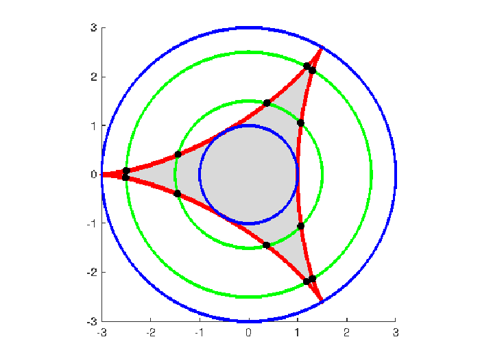
see Figure 1 Set , so that
For every fixed , let denote the roots of ordered with respect to magnitude. The set of norms of these roots is the image of under the exponential map. We would like to determine for which we have that . The lopsidedness certificate in this example implies that if
It follows from Corollary 6.3 that if is not contained in the region (6.3). Let us write . Then, by applying a Gröbner basis computation, the boundary of (6.3) is given by the hypocycloid
| (6.5) |
In particular, if , then . Notice that implies that , so our certificate is an improvement of the lopsidedness certificate. See Figure 1 for a comparison.
For example, if we require that then we obtain the following numerical intervals in the argument of which ensures that :
Similarly, if then we obtain the following numerical intervals:


Example 6.5.
Consider the family of bivariate polynomials
where . We associate to its homogeneous support set (see Remark 2.1) and a rational lift given by
| (6.6) |
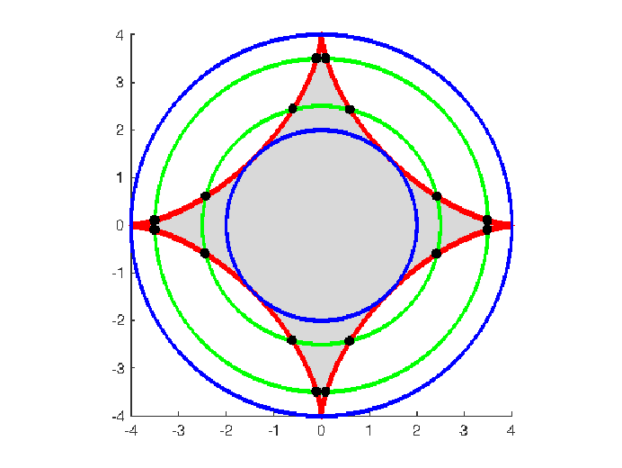
see Figure 2. Set , so that
By the lopsidedness criterion we can conclude that has a bounded component of order if . It follows from Corollary 6.3 that has a bounded component of order if is not contained in the region (6.3). Again, let us write . Then, the boundary of (6.3) is in this case given by the hypocycloid where
| (6.7) |
In particular, if , then has a bounded component of order . For example, if we require that then we obtain the following numerical intervals in the argument of which ensures the existence of a component of order :
Similarly, if then we obtain the following numerical intervals:


Corollary 6.3 is applicable also when . We leave the task of constructing an example for the curious reader, to keep the article at a reasonable length.
The fact that Theorem 6.2 requires a barycentric circuit is a serious restriction. For non-barycentric circuits the only known certificates are certain upper and lower bounds on the norms of the coefficients, see [17, Theorems 4.1 and 4.4]. Unfortunately, the lower bounds yields no new certificates in conjunction with Theorem 4.1. The upper bounds are equivalent to the lopsidedness criterion, see [17, Theorem 5.3].
We observed experimentally that a non-barycentric circuit polynomial with has a solid amoeba if and only if the coefficient of the term whose exponent corresponds to the interior point is not contained in a region bounded by a hypocycloid determined by the remaining coefficients. We believe that a similar statement as Theorem 4.1 holds for all circuits, this is the subject of an ongoing investigation.
References
- [1] M. Avendano, R. Kogan, M. Nisse, and J. Maurice Rojas, Metric estimates and membership complexity for archimedean amoebae and tropical hypersurfaces, arXiv:1307.3681, 2013.
- [2] T. de Wolff, Amoebas and their tropicalizations - a survey, Analysis Meets Geometry: The Mikael Passare Memory Volume (M. Andersson, J. Boman, C. Kiselman, P. Kurasov, and R. Sigurdsson, eds.), Trends in Mathematics, Birkhäuser, Basel, 2017, pp. 157–190.
- [3] S. Y. Favorov, Holomorphic almost periodic functions in tube domains and their amoebas, Comput. Methods Funct. Theory 1 (2001), no. 2, [On table of contents: 2002], 403–415.
- [4] M. Forsberg, M. Passare, and A. Tsikh, Laurent determinants and arrangements of hyperplane amoebas, Adv. Math. 151 (2000), no. 1, 45–70.
- [5] J. Forsgård, L. Matusevich, N. Mehlhop, and T. de Wolff, Lopsided approximation of amoebas, 2016, to appear in Math. Comp., see arXiv:1608.08663.
- [6] M. Fujiwara, Über die obere Schranke des absoluten Betrages der Wurzeln einer algebraischen Gleichung., Tohoku Math. J. 10 (1916), 167–171 (English; Japanese).
- [7] I. M. Gel’fand, M. M. Kapranov, and A. V. Zelevinsky, Discriminants, resultants and multidimensional determinants, Mathematics: Theory & Applications, Birkhäuser Boston, Inc., Boston, MA, 1994.
- [8] E. Landau, Sur quelques généralisations du théorème de M. Picard, Ann. Sci. École Norm. Sup. (3) 24 (1907), 179–201, in French.
- [9] D. Maclagan and B. Sturmfels, Introduction to Tropical Geometry, Amer. Math. Soc., Providence, R.I., 2015.
- [10] G. Mikhalkin, Amoebas of algebraic varieties and tropical geometry, Different Faces of Geometry (S. K. Donaldson, Y. Eliashberg, and M. Gromov, eds.), Kluwer, New York, 2004, pp. 257–300.
- [11] M. Passare and H. Rullgård, Amoebas, Monge-Ampére measures and triangulations of the Newton polytope, Duke Math. J. 121 (2004), no. 3, 481–507.
- [12] M. Passare and A. Tsikh, Amoebas: their spines and their contours, Idempotent mathematics and mathematical physics, Contemp. Math., vol. 377, Amer. Math. Soc., 2005, pp. 275–288.
- [13] K. Purbhoo, A Nullstellensatz for amoebas, Duke Math. J. 14 (2008), no. 3, 407–445.
- [14] H. Rullgård, Topics in geometry, analysis and inverse problems, Ph.D. thesis, Stockholm University, 2003.
- [15] D. Schleicher and R. Stoll, Newton’s method in practice: Finding all roots of polynomials of degree one million efficiently, Theoret. Comput. Sci. 681 (2017), 146–166.
- [16] J. Silipo, The Ronkin number of an exponential sum, Math. Nachr. 285 (2012), no. 8-9, 1117–1129.
- [17] T. Theobald and T. de Wolff, Amoebas of genus at most one, Adv. Math. 239 (2013), 190–213.
- [18] T. Theobald and T. de Wolff, Norms of roots of trinomials, Math. Ann. (2015), 1–29.