Safe and Resilient Multi-vehicle Trajectory Planning Under Adversarial Intruder
Abstract
Provably safe and scalable multi-vehicle trajectory planning is an important and urgent problem. Hamilton-Jacobi (HJ) reachability is an ideal tool for analyzing such safety-critical systems and has been successfully applied to several small-scale problems. However, a direct application of HJ reachability to multi-vehicle trajectory planning is often intractable due to the “curse of dimensionality.” To overcome this problem, the sequential trajectory planning (STP) method, which assigns strict priorities to vehicles, was proposed; STP allows multi-vehicle trajectory planning to be done with a linearly-scaling computation complexity. However, if a vehicle not in the set of STP vehicles enters the system, or even worse, if this vehicle is an adversarial intruder, the previous formulation requires the entire system to perform replanning, an intractable task for large-scale systems. In this paper, we make STP more practical by providing a new algorithm where replanning is only needed only for a fixed number of vehicles, irrespective of the total number of STP vehicles. Moreover, this number is a design parameter, which can be chosen based on the computational resources available during run time. We demonstrate this algorithm in a representative simulation of an urban airspace environment.
I Introduction
Recently, there has been an immense surge of interest in the use of unmanned aerial systems (UASs) for civil applications [1, 2, 3, 4, 5], which will involve unmanned aerial vehicles (UAVs) flying in urban environments, potentially in close proximity to humans, other UAVs, and other important assets. As a result, new scalable ways to organize an airspace are required in which potentially thousands of UAVs can fly together [6, 7].
One essential problem that needs to be addressed for this endeavor to be successful is that of trajectory planning: how a group of vehicles in the same vicinity can reach their destinations while avoiding situations which are considered dangerous, such as collisions. Many previous studies address this problem under different assumptions. In some studies, specific control strategies for the vehicles are assumed, and approaches such as those involving induced velocity obstacles [8, 9, 10, 11] and those involving virtual potential fields to maintain collision avoidance [12, 13] have been used. Methods have also been proposed for real-time trajectory generation [14], for path planning for vehicles with linear dynamics in the presence of obstacles with known motion [15], and for cooperative path planning via waypoints which do not account for vehicle dynamics [16]. Other related work is in the collision avoidance problem without path planning. These results include those that assume the system has a linear model [17, 18, 19], rely on a linearization of the system model [20, 21], assume a simple positional state space [22], and many others [23, 24, 25].
However, methods to flexibly plan provably safe and dynamically feasible trajectories without making strong assumptions on the vehicles’ dynamics and other vehicles’ motion are lacking. Moreover, any trajectory planning scheme that addresses collision avoidance must also guarantee both goal satisfaction and safety of UAVs despite disturbances and communication faults [7]. Furthermore, unexpected scenarios such as UAV malfunctions or even UAVs with malicious intent need to be accounted for. Finally, the proposed scheme should scale well with the number of vehicles.
Hamilton-Jacobi (HJ) reachability-based methods [26, 27, 28, 29, 30, 31] are particularly suitable in the context of UAVs because of the formal guarantees provided. In this context, one computes the reach-avoid set, defined as the set of states from which the system can be driven to a target set while satisfying time-varying state constraints at all times. A major practical appeal of this approach stems from the availability of modern numerical tools which can compute various definitions of reachable sets [32, 33, 34, 35]. These numerical tools, for example, have been successfully used to solve a variety of differential games, trajectory planning problems, and optimal control problems [36, 37, 38, 39]. However, reachable set computations involve solving a HJ partial differential equation (PDE) or variational inequality (VI) on a grid representing a discretization of the state space, resulting in an exponential scaling of computational complexity with respect to the system dimensionality. Therefore, reachability analysis or other dynamic programming-based methods alone are not suitable for managing the next generation airspace, which is a large-scale system with a high-dimensional joint state space because of the possible high density of vehicles that needs to be accommodated [7].
To overcome this problem, the priority-based Sequential Trajectory Planning (STP) method has been proposed [40, 41]. In this context, higher-priority vehicles plan their trajectories without taking into account the lower-priority vehicles, and lower-priority vehicles treat higher-priority vehicles as moving obstacles. Under this assumption, time-varying formulations of reachability [29, 31] can be used to obtain the optimal and provably safe trajectories for each vehicle, starting from the highest-priority vehicle. Thus, the curse of dimensionality is overcome at the cost of a structural assumption, under which the computation complexity scales just linearly with the number of vehicles. In addition, such a structure has the potential to flexibly divide up the airspace for the use of many UAVs and allows tractable multi-vehicle trajectory-planning. Practically, different economic mechanisms can be used to establish a priority order. One example could be first-come-first-serve mechanism, as highlighted in NASA’s concept of operations for UAS traffic management [7].
However, if a vehicle not in the set of STP vehicles enters the system, or even worse, if this vehicle has malicious intent, the original plan can lead to a vehicle colliding with another vehicle, leading to a domino effect, causing the entire STP structure to collapse. Thus, STP vehicles must plan with an additional safety margin that takes a potential intruder into account. The authors in [42] propose an STP algorithm that accounts for such a potential intruder. However, a new full-scale trajectory planning problem is required to be solved in real time to ensure safe transit of the vehicles to their respective destinations. Since the replanning must be done in real-time, the proposed algorithm in [42] is intractable for large-scale systems even with the STP structure. In this work, we propose a novel algorithm that limits the replanning to a fixed number of vehicles, irrespective of the total number of STP vehicles. Moreover, this design parameter can be chosen beforehand based on the computational resources available.
Intuitively, for every vehicle, we compute a separation region such that the vehicle needs to account for the intruder if and only if the intruder is inside this separation region. We then compute a buffer region between the separation regions of any two vehicles, and ensure that this buffer is maintained as vehicles are traveling to their destinations. Thus, to intrude every additional vehicle, the intruder must travel through the buffer region. Therefore, we can design the buffer region size such that the intruder can affect at most a specified number of vehicles within some duration. A high-level overview of the proposed algorithm is provided in Algorithm 1.
Vehicle dynamics and initial states;
Vehicle destinations and any obstacles to avoid;
Intruder dynamics;
: Maximum number of vehicles allowed to re-plan their trajectories.
Intruder avoidance and goal-satisfaction controller.
In Section II, we formalize the STP problem in the presence of disturbances and adversarial intruders. In Section III, we present an overview of time-varying reachability and basic STP algorithms in [40], [41]. In Section IV, we present our proposed algorithm. Finally, we illustrate this algorithm through a fifty-vehicle simulation in an urban environment in Section V. Notations are summarized in Table I.
II Sequential Trajectory Planning Problem
Consider vehicles (also denoted as STP vehicles) which participate in the STP process. We assume their dynamics are given by
| (1) | ||||
where , and , respectively, represent the state, control and disturbance experienced by vehicle . We partition the state into the position component and the non-position component : . We will use the sets to respectively denote the set of functions from which the control and disturbance functions are drawn.
Each vehicle has initial state , and aims to reach its target by some scheduled time of arrival . The target in general represents some set of desirable states, for example the destination of . On its way to , must avoid a set of static obstacles , which could represent any set of states, such as positions of tall buildings, that are forbidden. Each vehicle must also avoid the danger zones with respect to every other vehicle . For simplicity, we define the danger zone of with respect to to be
| (2) |
The danger zones in general can represent any joint configurations between and that are considered to be unsafe. In particular, and are said to have collided if .
In addition to the obstacles and danger zones, an intruder vehicle may also appear in the system. An intruder vehicle may have malicious intent or simply be a non-participating vehicle that could accidentally collide with other vehicles. This general definition of intruder allows us to develop algorithms that can also account for vehicles who are not communicating with the STP vehicles or do not know about the STP structure. In general, the effect of intruders on vehicles in structured flight can be unpredictable, since the intruders in principle could be adversarial in nature, and the number of intruders could be arbitrary, in which case a collision avoidance problem must be solved for each STP vehicle in the joint state-space of all intruders and the STP vehicle. Therefore, to make our analysis tractable, we make the following two assumptions.
Assumption 1
At most one intruder affects the STP vehicles at any given time. The intruder is removed after a duration of .
This assumption can be valid in situations where intruders are rare, and that some fail-safe or enforcement mechanism exists to force the intruder out of the planning space. For example, when STP vehicles are flying at a particular altitude level, the removal of the intruder can be achieved by forcing the intruder to exit the altitude level. Practically, over a large region of the unmanned airspace, this assumption implies that there would be one intruder vehicle per “planning region”. Each planning region would perform STP independently from the others. One would design planning regions to be an appropriate size such that it is reasonable to assume at most one intruder would appear. The entire large region would be composed of several planning regions.
Let the time at which intruder appears in the system be . Assumption 1 implies that any vehicle would need to avoid the intruder for a maximum duration of . Note that we do not pose any restriction on ; we only assume that once the intruder appears, it stays for a maximum duration of .
Assumption 2
The dynamics of the intruder are known and given by .
Assumption 2 is required for HJ reachability analysis. In situations where the dynamics of the intruder are not known exactly, a conservative model of the intruder may be used instead. We also denote the initial state of the intruder as Note that we only assume that the dynamics of the intruder are known, but its initial state , control and disturbance it experiences are unknown.
Given the set of STP vehicles, their targets , the static obstacles , the vehicles’ danger zones with respect to each other , and the intruder dynamics , our goal is as follows. For each vehicle , synthesize a controller which guarantees that reaches its target at or before the scheduled time of arrival , while avoiding the static obstacles , the danger zones with respect to all other vehicles , and the intruder vehicle , irrespective of the control strategy of the intruder. In addition, we would like to obtain the latest departure time such that can still arrive at on time.
Due to the high dimensionality of the joint state-space, a direct dynamic programming-based solution is intractable. Therefore, the authors in [40] proposed to assign a priority to each vehicle, and perform STP given the assigned priorities. Without loss of generality, let have a higher-priority than if . Under the STP scheme, higher-priority vehicles can ignore the presence of lower-priority vehicles, and perform trajectory planning without taking into account the lower-priority vehicles’ danger zones. A lower-priority vehicle , on the other hand, must ensure that it does not enter the danger zones of the higher-priority vehicles or the intruder vehicle ; each higher-priority vehicle induces a set of time-varying obstacles , which represents the possible states of such that a collision between and or and could occur.
It is straightforward to see that if each vehicle is able to plan a trajectory that takes it to while avoiding the static obstacles , the danger zones of higher-priority vehicles , and the danger zone of the intruder , then the set of STP vehicles would all be able to reach their targets safely. Under the STP scheme, trajectory planning can be done sequentially in descending order of vehicle priority in the state space of only a single vehicle. Thus, STP provides a solution whose complexity scales linearly with the number of vehicles. It is important to note that the trajectory planning is always feasible for the lower-priority vehicle under STP because a lower-priority vehicle can always depart early to avoid the higher-priority vehicle on its way to its destination.
When an intruder appears in the system, STP vehicles may need to avoid the intruder to ensure safety. Depending on the initial state of the intruder and its control policy, a vehicle will potentially need to apply different avoidance controls leading to different final states after avoiding the intruder. Therefore, a vehicle’s control policy that ensures its successful transit to its destination needs to account for all such possible final states, which is a trajectory planning problem with multiple initial states and a single destination, and is hard to solve in general. Thus, we divide the intruder avoidance problem into two sub-problems: (i) we first design a control policy that ensures a successful transit to the destination if no intruder appears and that successfully avoids the intruder otherwise (Algorithm 1). (ii) After the intruder disappears from the system, we replan the trajectories of the affected vehicles. Following the same theme and assumptions, the authors in [42] present an algorithm to avoid an intruder in STP formulation; however, in the worst-case, the algorithm might need to replan the trajectories for all STP vehicles. Our goal in this work is to present an algorithm that ensures that only a small and fixed number of vehicles needs to replan their trajectories, regardless of the total number of vehicles, resulting in a constant replanning time. In particular, we answer the following inter-dependent questions:
- 1.
How can each vehicle guarantee that it will reach its target set without getting into any danger zones, despite no knowledge of the intruder initial state, the time at which it appears, its control strategy, and disturbances it experiences?
- 2.
How can we ensure that replanning only needs to be done for at most a chosen fixed maximum number of vehicles after the intruder disappears from the system?
| Notation | Description | Location | Interpretation |
|---|---|---|---|
| Buffer region between vehicle and vehicle | Beginning of Section IV-B2 | The set of all possible states for which the separation requirement may be violated between vehicle and vehicle for some intruder strategy. If vehicle is outside this set, then the intruder will need atleast a duration of to go from the avoid region of vehicle to the avoid region of vehicle . | |
| Disturbance in the dynamics of vehicle | Beginning of Section II | - | |
| Disturbance in the dynamics of the intruder | Assumption 2 | - | |
| Dynamics of vehicle | Beginning of Section II | - | |
| Dynamics of the intruder | Assumption 2 | - | |
| Relative dynamics between two vehicles | Equation (12) | - | |
| The overall obstacle for vehicle | Equation (7) | The set of states that vehicle must avoid on its way to the destination. | |
| Non-position state component of vehicle | Beginning of Section II | - | |
| - | Beginning of Section IV | The maximum number of vehicles that should apply the avoidance maneuver or the maximum number of vehicles that we can replan trajectories for in real-time. | |
| Target set of vehicle | Beginning of Section II | The destination of vehicle . | |
| Base obstacle induced by vehicle at time | Equations (25), (31) and (37) in [42] | The set of all possible states that vehicle can be in at time if the intruder does not appear in the system till time . | |
| Number of STP vehicles | Beginning of Section II | - | |
| - | Equation (39) | The set of vehicles that need to replan their trajectories after the intruder disappears. These are also the set of vehicles that were forced to apply an avoidance maneuver. | |
| Induced obstacle by vehicle for vehicle | After Assumption 2 in Section II | The possible states of vehicle such that a collision between vehicle and vehicle or vehicle and the intruder vehicle (if present) could occur. | |
| Static obstacle for vehicle | Beginning of Section II | Obstacles that vehicle needs to avoid on its way to destination, e.g, tall buildings. | |
| Position of vehicle | Beginning of Section II | - | |
| th STP vehicle | Beginning of Section II | - | |
| The intruder vehicle | Assumption 1 | - | |
| Danger zone radius | Equation (2) | The closest distance between vehicle and vehicle that is considered to be safe. | |
| Separation region of vehicle at time | Beginning of Section IV-B1 | The set of all states of intruder at time for which vehicle is forced to apply an avoidance maneuver. | |
| Avoid start time of vehicle | Equation (18) | The first time at which vehicle is forced to apply an avoidance maneuver by the intruder vehicle. Defined to be if vehicle never applies an avoidance maneuver. | |
| Buffer region travel duration | Beginning of Section IV | The minimum time required for the intruder to travel through the buffer region between any pair of vehicles. | |
| Intruder avoidance time | Assumption 1 | The maximum duration for which the intruder is present in the system. | |
| Intruder appearance time | After Assumption 1 | The time at which the intruder appears in the system. | |
| Latest departure time of vehicle | End of Section II | The latest departure time for vehicle such that it safely reaches its destination by the scheduled time of arrival. | |
| Scheduled time of arrival (STA) of vehicle | Beginning of Section II | The time by which vehicle is required to reach its destination. | |
| Control of vehicle | Beginning of Section II | - | |
| Control of the intruder | Assumption 2 | - | |
| Optimal avoidance control of vehicle | Equation (15) | The control that vehicle need to apply to successfully avoid the intruder once the relative state between vehicle and the intruder reaches the boundary of the avoid region of vehicle . | |
| Nominal control | Equation (37) | The nominal control for vehicle that will ensure its successful transition to its destination if the intruder does not force it to apply an avoidance maneuver. This control law corresponds to the nominal trajectory of vehicle . | |
| The overall controller for vehicle | Equation (40) | The overall controller for vehicle that will ensure a successful and safe transit to its destination despite the worst-case intruder strategy. | |
| Avoid region of vehicle | Equation (13) | The set of relative states for which the intruder can force vehicle to enter in the danger zone within a duration of . | |
| Relative buffer region | Beginning of Section IV-B2 | The set of all states from which it is possible to reach the boundary of the avoid region of vehicle within a duration of . | |
| - | Equation (35) | The set of all states that vehicle needs to avoid in order to avoid a collision with the static obstacles while applying an avoidance maneuver. | |
| - | Equation (32) | The set of all initial states of vehicle from which it is guaranteed to safely reach its destination if the intruder does not force it to apply an avoidance maneuver and successfully and safely avoid the intruder in case needs it does. | |
| State of vehicle | Beginning of Section II | - | |
| State of the intruder vehicle | Assumption 2 | - | |
| Initial state of vehicle | Beginning of Section II | - | |
| Initial state of the intruder vehicle | Assumption 2 | - | |
| Relative state between the intruder and vehicle | Equation (12) | - | |
| Danger zone between vehicle and vehicle | Equation (2) | Set of all states of vehicle and vehicle which are within unsafe distance of each other. The vehicles are said to have collided if their states belong to . |
III Background
In this section, we first present the basic STP algorithm [40] in which disturbances and the intruders are ignored and perfect information of vehicles’ positions is assumed. We then briefly discuss the different algorithms proposed in [41] to account for disturbances in vehicles’ dynamics. All of these algorithms use time-varying reachability analysis to provide goal satisfaction and safety guarantees; therefore, we start with an overview of time-varying reachability.
III-A Time-Varying Reachability Background
We will be using reachability analysis to compute either a backward reachable set (BRS) , a forward reachable set (FRS) , or a sequence of BRSs and FRSs, given some target set , time-varying obstacle which captures trajectories of higher-priority vehicles, and the Hamiltonian function which captures the system dynamics as well as the roles of the control and disturbance. The BRS in a time interval or FRS in a time interval will be denoted by or respectively. Typically, when computing the BRS, will be some fixed final time, for example the scheduled time of arrival . When computing the FRS, will be some fixed initial time, for example the starting time or the present time.
Several formulations of reachability are able to account for time-varying obstacles [29, 31] (or state constraints in general). For our application in STP, we utilize the formulation in [31], in which a BRS is computed by solving the following final value double-obstacle HJ VI:
| (3) | ||||
In a similar fashion, the FRS is computed by solving the following initial value HJ PDE:
| (4) | ||||
In both (3) and (4), the function is the implicit surface function representing the target set . Similarly, the function is the implicit surface function representing the time-varying obstacles . The BRS and FRS are given by
| (5) | ||||
Some of the reachability computations will not involve an obstacle set , in which case we can simply set which effectively means that the outside maximum is ignored in (3). Also, note that unlike in (3), there is no inner minimization in (4). As we will see later, we will be using the BRS to determine all states that can reach some target set within the time horizon , whereas we will be using the FRS to determine where a vehicle could be at some particular time .
The Hamiltonian, , depends on the system dynamics, and the role of control and disturbance. Whenever does not depend explicitly on , we will drop from the argument. In addition, the optimization of Hamiltonian gives the optimal control and optimal disturbance , once is determined. For BRSs, whenever the existence of a control (“”) or disturbance is sought, the optimization is a minimum over the set of controls or disturbance. Whenever a BRS characterizes the behavior of the system for all controls (“”) or disturbances, the optimization is a maximum. We will introduce precise definitions of reachable sets, expressions for the Hamiltonian, expressions for the optimal controls as needed for the many different reachability calculations we use.
III-B STP Without Disturbances and Intruder
In this section, we give an overview of the basic STP algorithm assuming that there is no disturbance and no intruder affecting the vehicles. The majority of the content in this section is taken from [40].
Recall that among the STP vehicles , has a higher priority than if . In the absence of disturbances, we can write the dynamics of the STP vehicles as
| (6) |
In STP, each vehicle plans its trajectory while avoiding static obstacles and the obstacles induced by higher-priority vehicles . Trajectory planning is done sequentially in descending priority, . During its trajectory planning process, ignores the presence of lower-priority vehicles . From the perspective of , each of the higher-priority vehicles induces a time-varying obstacle denoted that needs to avoid. Therefore, each vehicle must plan its trajectory while avoiding the union of all the induced obstacles as well as the static obstacles. Let be the union of all the obstacles that must avoid on its way to :
| (7) |
With full position information of higher-priority vehicles, the obstacle induced for by is simply
| (8) |
Each higher-priority vehicle ignores . Since trajectory planning is done sequentially in descending order of priority, the vehicles would have planned their trajectories before does. Thus, in the absence of disturbances, is a priori known, and therefore are known, deterministic moving obstacles, which means that is also known and deterministic. Therefore, the trajectory planning problem for can be solved by first computing the BRS , defined as follows:
| (9) | ||||
The BRS can be obtained by solving (3) with , , and the Hamiltonian
| (10) |
The optimal control for reaching while avoiding is then given by
| (11) |
from which the trajectory can be computed by integrating the system dynamics, which in this case are given by (6). In addition, the latest departure time can be obtained from the BRS as . The basic STP algorithm is summarized in Algorithm 2.
III-C STP With Disturbances and Without Intruder
Disturbances and incomplete information significantly complicate the STP scheme. The main difference is that the vehicle dynamics satisfy (1) as opposed to (6). Committing to exact trajectories is therefore no longer possible, since the disturbance is a priori unknown. Thus, the induced obstacles are no longer just the danger zones centered around positions, unlike in (8). In particular, a lower-priority vehicle needs to account for all possible states that the higher-priority vehicles could be in. To do this, the lower-priority vehicle needs to have some knowledge about the control policy used by each higher-priority vehicle. Three different methods are presented in [41] to address the above issues. The methods differ in terms of control policy information that is known to a lower-priority vehicle.
- •
Centralized control: A specific control strategy is enforced upon a vehicle; this can be achieved, for example, by some central agent such as an air traffic controller.
- •
Least restrictive control: A vehicle is required to arrive at its targets on time, but has no other restrictions on its control policy. When the control policy of a vehicle is unknown, the least restrictive control can be safely assumed by lower-priority vehicles.
- •
Robust trajectory tracking: A vehicle declares a nominal trajectory which can be robustly tracked under disturbances.
In each case, a vehicle can compute all possible states that a higher-priority vehicle can be in based on the control strategy information known to the lower priority vehicle. A collision avoidance between and is thus ensured. We refer to the obstacle , induced in the presence of disturbances but in the absence of intruders, as base obstacle and denote it as from here on. Further details of each algorithm are presented in [41].
IV Response to Intruders
In this section, we propose a method to allow vehicles to avoid an intruder while maintaining the STP structure. Our goal is to design a control policy for each vehicle that ensures separation with the intruder and other STP vehicles, and ensures a successful transit to the destination.
As discussed in Section II, depending on the initial state of the intruder and its control policy, a vehicle may arrive at different states after avoiding the intruder. To make sure that the vehicle still reaches its destination, a replanning of vehicle’s trajectory is required. Since the replanning must be done in real-time, we also need to ensure that only a small number of vehicles require replanning. In this work, a novel intruder avoidance algorithm is proposed, which will need to replan trajectories only for a small fixed number of vehicles, irrespective of the total number of STP vehicles. Moreover, this number is a design parameter, which can be chosen based on the resources available during run time.
Let denote the maximum number of vehicles that we can replan the trajectories for in real-time. Also, let . We divide our algorithm in two parts: the planning phase and the replanning phase. In the planning phase, our goal is to divide the flight space of vehicles such that at any given time, any two vehicles are far enough from each other so that an intruder needs at least a duration of to travel from the vicinity of one vehicle to that of another. Since the intruder is present for a total duration of , this division ensures that it can only affect at most vehicles despite its best efforts. In particular, we compute a separation region for each vehicle such that the vehicle needs to account for the intruder if and only if the intruder is inside this separation region. We then compute a buffer region between the separation regions of any two vehicles such that the intruder requires atleast a duration of to travel through this region. A high-level overview of the planning phase is presented in Algorithm 1. The planning phase ensures that after the intruder disappears, at most vehicles have to replan their trajectories. In the replanning phase, we re-plan the trajectories of affected vehicles so that they reach their destinations safely.
Note that our theory assumes worst-case scenarios in terms of the behavior of the intruder, the effect of disturbances, and the planned trajectories of each STP vehicle. This way, we are able to guarantee safety and goal satisfaction of all vehicles in all possible scenarios given the bounds on intruder dynamics and disturbances. To achieve denser operation of STP vehicles, known information about the intruder, disturbances, and specifies of STP vehicle trajectories may be incorporated; however, these considerations are out of the scope of this paper.
The rest of the section is organized as follows. In Sections IV-A, we discuss the intruder avoidance control that a vehicle needs to apply within the separation region. In Sections IV-B and IV-C, we compute the separation and buffer regions for vehicles. Trajectory planning that maintains the buffer region between every pair of vehicles is discussed in Section IV-D. Finally, the replanning of the trajectories of the affected vehicles is discussed in Section IV-E.
IV-A Optimal Avoidance Controller
In this section, our goal is to compute the control policy that a vehicle can use to avoid entering in the danger region . We also compute the set of states from which the joint states of and can enter the danger zone despite the best efforts of to avoid , which is then used to compute the separation region of in Section IV-B1.
We define relative dynamics of the intruder with state with respect to with state :
| (12) |
Given the relative dynamics, the set of states from which the joint states of and can enter danger zone in a duration of despite the best efforts of to avoid is given by the backward reachable set :
| (13) | ||||
The Hamiltonian to compute is given as:
| (14) |
We refer to as avoid region from here on. The interpretation of is that if starts inside this set, i.e., , then the intruder can force to enter the danger zone within a duration of , regardless of the control applied by the vehicle. If starts at the boundary of this set (denoted as ), i.e., , it can barely successfully avoid the intruder for a duration of using the optimal avoidance control (referred to as avoidance maneuver from here on)
| (15) |
Finally, if starts outside this set, i.e., , then and cannot instantaneously enter the danger zone , irrespective of the control applied by them at time . In fact, can safely apply any control as long as it is outside the boundary of this set, but will have to apply the avoidance maneuver to avoid the intruder once it reaches the boundary.
In the worst case, might need to avoid the intruder for a duration of starting at ; thus, the least we must have is that to ensure successful avoidance. Otherwise, regardless of what control a vehicle applies, the intruder can force it to enter the danger zone .
Assumption 3
.
Intuitively, assumption 3 enforces a condition on the detection of the intruder by STP vehicles. For example, if STP vehicles are equipped with circular sensors, then assumption 3 implies that STP vehicle must be able to detect a intruder that is within a distance of , where
| (16) |
otherwise, there exists an intruder control strategy such that and will collide irrespective of the control used by . Thus, is the minimum detection range required by any trajectory-planning algorithm to ensure a successful intruder avoidance for all intruder strategies. In general, assumption 3 is required to ensure that the intruder gives the STP vehicles “a chance” to react and avoid it. Hence, for analysis to follow, we assume that assumption 3 holds.
Note that although (15) gives us a provably successful avoidance control for avoiding the intruder if , the vehicle may not be able to apply this control because it may lead to a collision with other STP vehicles. Thus, in general, assumption 3 is only necessary not sufficient to guarantee intruder avoidance. However, we ensure that the STP vehicles are always separated enough from each other so that any vehicle can apply avoidance maneuver if need be. Thus, for the proposed algorithm, assumption 3 will also be sufficient for a successful intruder avoidance.
IV-B Separation and Buffer Regions - Case 1
In the next two sections, our goal is to compute separation and buffer regions for STP vehicles so that at most vehicles are forced to apply an avoidance maneuver during the duration .
Intuitively, we divide the duration of into intervals and ensure that atmost one vehicle can be forced to apply the avoidance maneuver during each interval. Thus, by construction, it is guaranteed that at most vehicles apply the avoidance maneuver during the time interval . We refer to this structure as the separation requirement from here on. To ensure this requirement, we use the reachability theory to find the set of all states of such that the separation requirement can be violated between the vehicle pair , , at time . During the trajectory planning of , we then ensure that the vehicle is not in one of these states at time by using this set of states as “obstacle”. The sequential trajectory planning will therefore guarantee that the separation requirement holds for every STP vehicle pair.
Mathematically, we define
| (17) |
and the avoid start time
| (18) |
By definition of , is the set of all times at which must apply an avoidance maneuver and denotes the first such time. The separation requirement can thus be written as
| (19) |
The separation requirement essentially implies that the intruder requires a time duration of atleast before it can force any additional vehicle to apply an avoidance maneuver. Thus, any two STP vehicles should be “separated” enough from each other at any given time for such a requirement to hold.
We now focus on finding what that “separation set” (also referred to as the buffer region) between . Since the path planning is done in a sequential order, we assume that we have already planned a path for and compute the buffer region that needs to maintain to ensure that the separation requirement is satisfied. For this computation, it is sufficient to consider the following two mutually exclusive and exhaustive cases:
- 1.
Case 1:
- 2.
Case 2:
In this section, we consider Case 1. Case 2 is discussed in the next section.
In Case 1, the intruder forces , the higher-priority vehicle, to apply avoidance control before or at the same time as , the lower-priority vehicle. To ensure the separation requirement in this case, we begin with the following observation which narrows down the intruder scenarios that we need to consider:
Observation 1
Without loss of generality, we can assume that the intruder appears in the system at the boundary of the avoid region of , i.e., . Equivalently, we can assume that .
Since , reaches the boundary of the avoid region of before it reaches the boundary of the avoid region of . Furthermore, by the definition of the avoid region, vehicles and need not account for the intruder until it reaches the boundary of the avoid region of . Thus, it is sufficient to consider the worst case .
IV-B1 Separation region
Recall that the separation region denotes the set of states of the intruder for which a vehicle is forced to apply an avoidance maneuver. In this section our goal is to find , the separation region of at the avoid start time. By virtue of Observation 1, we will use and interchangeably here on.
As discussed in Section IV-A, needs to apply avoidance maneuver at time only if . To compute set , we thus need to translate these relative states to a set in the state space of the intruder. Therefore, if all possible states of at time are known, then can be trivially computed.
Recall from Section III-C that the base obstacle at time represents all possible states of at time , if the intruder doesn’t appear in the system until that time. This is precisely the set that we are interested in to compute the separation region. Depending on the information known to a lower-priority vehicle about ’s control strategy, we can use one of the three methods described in Section 5 in [42] (and Section III-C of this paper) to compute the base obstacles . In particular, the base obstacles are respectively given by equations (25), (31) and (37) in [42] for the centralized control, the least restrictive control and the robust trajectory tracking algorithms (the three proposed algorithms to account for disturbances in STP). We will explain the computation of the base obstacles further in Section IV-D.
IV-B2 Buffer Region
We are now ready to compute the buffer region , the set of states for which the separation requirement can be violated between the vehicle pair . Conversely, if is outside the buffer region, the separation requirement is satisfied between . We start with recalling the following three results/facts
To compute , we first compute , the set of all states that can reach the set within a duration of . Ensuring that the intruder is outside this set at time guarantees that it will need a duration of atleast before it can force to apply an avoidance maneuver (equivalently, reach the avoid region of ). Since the possible states of the intruder at is given by , we thus simply need to ensure that is outside . Thus, the minimum buffer region is given by:
| (21) |
We refer to as the relative buffer region here on, which is given by the following BRS:
| (22) | ||||
The Hamiltonian to compute is given by:
| (23) |
Intuitively, represents the set of all relative states from which it is possible to reach the boundary of within a duration of . Note that we use instead of as the target set for our computation above because the BRS is computed using the relative state (and not .)
To summarize, we can ensure that as long as . This will be ensured by using as an obstacle during the path planning of (see Section IV-D). Consequently, can force at most vehicles to apply an avoidance maneuver during a duration of .
IV-B3 Obstacle Computation
In Sections IV-B1 and IV-B2, we computed a buffer region between and such that the separation requirement is satisfied. However, it still needs to be ensured that a vehicle does not collide with other vehicles while applying an avoidance maneuver. In this section, we find the set of states that needs to avoid to avoid accidentally entering in during an avoidance maneuver. Since the trajectory planning is done in a sequential fashion, being a lower priority vehicle, also needs to avoid the states that can lead it to while is avoiding the intruder. These sets of states are then used as obstacles during the path planning of , which ensures that it never enters these “potentially unsafe” states.
To find this obstacle set, we consider the following two exhaustive cases:
- 1.
Case A: The intruder affects , but not , i.e., and .
- 2.
Case B: The intruder first affects and then , i.e., .
For each case, we compute the set of states that needs to avoid at time to avoid entering in eventually. Let and denote the corresponding sets of “obstacles” for the two cases. We begin with the following observation:
Observation 2
To compute obstacles at time , it is sufficient to consider the scenarios where . This is because if , then and/or will already be in the replanning phase at time (see assumption 1) and hence the two vehicles cannot be in conflict at time . On the other hand, if , then wouldn’t apply any avoidance maneuver at time .
- •
Case A: In this case, only applies an avoidance maneuver; therefore, should avoid the set of states that can lead to a collision with at time while is applying an avoidance maneuver. Note that since (by Observation 1), is given by the states that can reach while avoiding the intruder, starting from some state in the base obstacle, . These states can be obtained by computing a FRS from the base obstacles.
(24) represents the set of all possible states that can reach after a duration of starting from inside . This FRS can be obtained by solving the HJ VI in (4) with the following Hamiltonian:
(25) Since , the induced obstacles in this case can be obtained as:
(26) Observation 3
Since the base obstacles represent all possible states of a vehicle in the absence of an intruder, the base obstacle at any time is contained within the FRS of the base obstacle at any earlier time , computed forward for a duration of That is, , where , as before, denotes the FRS of computed forward for a duration of . The same argument can be applied to the FRSs computed from two different base obstacles and , i.e., if .
- •
Case B: In this case, first applies an avoidance maneuver followed by . Once starts applying avoidance control at time , it might deviate from its pre-planned control strategy. From the perspective of , can apply any control during . Furthermore, itself must apply avoidance maneuver during . Thus, the main challenge in this case is to ensure that and do not enter into even when both vehicles are applying avoidance maneuver and hence can apply any control from each other’s perspective. Thus at time , not only needs to avoid the states that could be in at time , but also all the states that could lead it to in future under some control actions of and . To compute this set of states, we make the following key observation:
Observation 4
For computing , it is sufficient to consider . If , then is not applying any avoidance maneuver at time and hence should only avoid the states that could be in at time . However, this is already ensured during computation of . If , then for a given , still needs to avoid the same set of states at time that it would have if .
Due to the separation and buffer regions, we have . This along with Observation 4 implies that . Also, from Observation 2, we have . Thus, . Since the intruder is present for a maximum duration of , might be applying any control during from the perspective of . In particular, for any given , can reach any state in at time , starting from some state in at time . Here, represents the FRS of computed forward for a duration of and is given by (24).
Taking into account all possible , is contained in the set:
(28) at time , where the upper bound on corresponds to the upper bound on . From Observation 3, we have for all . Therefore, .
From the perspective of , it needs to avoid all states at time that can reach for some control action of during time duration . This will ensure that and will not enter into each other’s danger zones regardless of the avoidance maneuver applied by them. This set of states is given by the following BRS:
(29) where
The Hamiltonian to compute is given by
(30) Finally, the induced obstacle in this case is given by
(31)
IV-C Separation and Buffer Regions - Case 2
We now consider Case 2: . In this case, the intruder forces , the lower-priority vehicle, to apply avoidance control before , the higher-priority vehicle. The separation region, the buffer region and the obstacles in this case can be computed in a similar manner to that in Case 1. The buffer region in this case is denoted as to differentiate it from Case 1 (i.e., the order of and indexes has been switched). Similarly, the obstacles for Case 2 are denoted as and , corresponding to the two cases similar to that in Section (IV-B3). For brevity purposes, this computation is presented in the Appendix.
IV-D Trajectory Planning
In this section, our goal is to plan the trajectory of each vehicle such that it is guaranteed to safely reach its target in the absence of an intruder, and to ensure collision avoidance with vehicles or obstacles if forced to apply an avoidance maneuver. We also need to make sure that the trajectories of the vehicles are such that the separation requirement is satisfied at all times. To obtain such a trajectory, we take into account all the “obstacles” computed in previous sections which ensure that the vehicle will not collide with any other vehicle, as long as it is outside these obstacles.
Before, we plan such a trajectory, we need to compute one final set of obstacles. In particular, we need to compute the set of states states that needs to avoid in order to avoid a collision with static obstacles while it is applying an avoidance maneuver. Since applies avoidance maneuver for a maximum duration of , this set is given by the following BRS:
| (32) | ||||
The Hamiltonian to compute is given by:
| (33) |
represents the set of all states of at time that can lead to a collision with a static obstacle for some time for some control strategy of .
During the trajectory planning of , if we use and as obstacles at time , then the separation requirement is ensured between and for all intruder strategies and . Similarly, if obstacles computed in sections IV-B3 and IV-C are used as obstacles in trajectory planning, then we can guarantee collision avoidance between and while they are avoiding the intruder. Thus, the overall obstacle for is given by:
| (34) | ||||
Given , we compute a BRS for trajectory planning that contains the initial state of and avoids these obstacles:
| (35) | ||||
The Hamiltonian to compute the BRS in (35) is given by:
| (36) |
Note that ensures goal satisfaction for in the absence of intruder. The goal satisfaction controller is given by:
| (37) |
When intruder is not present in the system, applies the control and we get the “nominal trajectory” of . Once intruder appears in the system, applies the avoidance control and hence might deviate from its nominal trajectory. The overall control policy for avoiding the intruder and collision with other vehicles is thus given by:
| (38) |
If starts within and uses the control , it is guaranteed to avoid collision with the intruder and other STP vehicles, regardless of the control strategy of . Finally, since we use separation and buffer regions as obstacles during the trajectory planning of , it is guaranteed that for all . Therefore, atmost vehicles are forced to apply an avoidance maneuver. The planning phase is summarized in Algorithm 3.
Remark 1
Note that given and , the base obstacles required for the computation of the separation region in Section IV-B1 can be computed using equations (25), (31) and (37) in [42]. Also, if we use the robust trajectory tracking method to compute the base obstacles, we would need to augment the obstacles in (34) by the error bound of , (for details, see Section 5A-3 in [42]). The BRS in (35) in this case is computed assuming no disturbance in ’s dynamics.
Vehicle destinations and static obstacles ;
Intruder dynamics and the maximum avoidance time ;
Maximum number of vehicles allowed to re-plan their trajectories .
IV-E Replanning after intruder avoidance
As discussed in Section IV-D, the intruder can force some STP vehicles to deviate from their planned nominal trajectory; therefore, goal satisfaction is no longer guaranteed once a vehicle is forced to apply an avoidance maneuver. Therefore, we have to replan the trajectories of these vehicles once disappears. The set of all vehicles for whom replanning is required, , can be obtained by checking if a vehicle applied any avoidance control during , i.e.,
| (39) |
Note that due to the presence of separation and buffer regions, at most vehicles can be affected by , i.e., . Goal satisfaction controllers which ensure that these vehicles reach their destinations can be obtained by solving a new STP problem, where the starting states of the vehicles are now given by the states they end up in, denoted , after avoiding the intruder. Note that we can pick beforehand and design buffer regions accordingly. Thus, by picking compatible based on the available computation resources during run-time, we can ensure that this replanning can be done in real time. Moreover, flexible trajectory-planning algorithms such as FaSTrack [43] can be used that can perform replanning efficiently in real-time.
Let the optimal control policy corresponding to this liveness controller be denoted . The overall control policy that ensures intruder avoidance, collision avoidance with other vehicles, and successful transition to the destination for vehicles in is given by:
| (40) |
Note that in order to re-plan using a STP method, we need to determine feasible for all vehicles. This can be done by computing an FRS:
| (41) | ||||
where represents the state of at ; takes into account the fact that now needs to avoid all other vehicles in and is defined in a way analogous to (7). The FRS in (41) can be obtained by solving
| (42) | ||||
where represent the FRS, obstacles during re-planning, and the initial state of , respectively. The new of is now given by the earliest time at which intersects the target set , . Intuitively, this means that there exists a control policy which will steer the vehicle to its destination by that time, despite the worst case disturbance it might experience. The replanning phase is summarized in Algorithm 4.
Remark 2
Note that even though we have presented the analysis for one intruder, the proposed method can handle multiple intruders as long as only one intruder is present at any given time.
Vehicle dynamics (1) and new initial states ;
Vehicle destinations and static obstacles ;
Total base obstacle set induced by all other vehicles in .
V Simulations
We now illustrate the proposed algorithm using a fifty-vehicle example.
V-A Setup
Our goal is to simulate a scenario where UAVs are flying through an urban environment. This setup can be representative of many UAV applications, such as package delivery, aerial surveillance, etc. For this purpose, we use the city of San Francisco (SF), California, USA as our planning region, as shown in Figure 1. Practically speaking, depending on the UAV density, it may be desirable to have smaller planning regions that together cover the SF area; however, such considerations are out of the scope of this paper.

Each box in Figure 1 represents a area of SF. The origin point for the vehicles is denoted by the Blue star. Four different areas in the city are chosen as the destinations for the vehicles. Mathematically, the target sets of the vehicles are circles of radius in the position space, i.e. each vehicle is trying to reach some desired set of positions. In terms of the state space , the target sets are defined as , where are centers of the target circles. The four targets are represented by four circles in Figure 1. The destination of each vehicle is chosen randomly from these four destinations. Finally, tall buildings in downtown San Francisco are used as static obstacles, denoted by black contours in Figure 1. We use the following dynamics for each vehicle:
| (43) | ||||
where is the state of vehicle , is the position and is the heading. represents ’s disturbances, for example wind, that affect its position evolution. The control of is , where is the speed of and is the turn rate; both controls have a lower and upper bound. To make our simulations as close as possible to real scenarios, we choose velocity and turn-rate bounds as , , , aligned with the modern UAV specifications [44, 45]. The disturbance bound is chosen as , which corresponds to moderate winds on the Beaufort wind force scale [46]. Note that we have used same dynamics and input bounds across all vehicles for clarity of illustration; however, our method can easily handle more general systems of the form in which the vehicles have different control bounds and dynamics.
The goal of the vehicles is to reach their destinations while avoiding a collision with the other vehicles or the static obstacles. The vehicles also need to account for the possibility of the presence of an intruder for a maximum duration of , whose dynamics are given by (43). The joint state space of this fifty-vehicle system is 150-dimensional (150D); therefore, we assign a priority order to vehicles and solve the trajectory planning problem sequentially. For this simulation, we assign a random priority order to fifty vehicles and use the algorithm proposed in Section IV to compute a separation between STP vehicles so that they do not collide with each other or the intruder.
V-B Results
In this section, we present the simulation results for ; occasionally, we also compare the results for different values of to highlight some key insights about the proposed algorithm. As per Algorithm 3, we begin with computing the avoid region . To compute the avoid region, relative dynamics between and are required. Given the dynamics in (43), the relative dynamics are given by [27]:
| (44) | ||||
where is the relative state between and . Given the relative dynamics, the avoid region can be computed using (13). For all the BRS and FRS computations in this simulation, we use Level Set Toolbox [35]. Also, since the vehicle dynamics are same across all vehicles, we will omit the vehicle index from sets wherever applicable. The avoid region for STP vehicles is shown in the top-right plot of Figure 2.
As long as starts outside the avoid region, is guaranteed to be able to avoid the intruder for a duration of . Given , we can compute the minimum required detection range given by (16) for the circular sensors, which turns out to be in this case, corresponding to a detection of in advance (given the speed of ). So as long as the vehicles can detect the intruder within , the proposed algorithm guarantees collision avoidance with the intruder as well as a safe transit to their respective destinations.
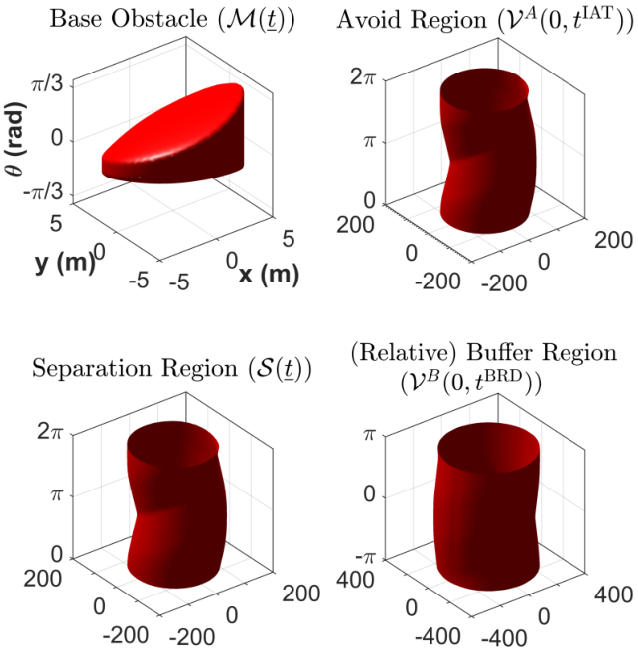
Next, we compute the separation and buffer regions between vehicles. For the computation of base obstacles, we use RTT method [41]. In RTT method, a nominal trajectory is declared by the higher-priority vehicles, which is then guaranteed to be tracked with some known error bound in the presence of disturbances. The base obstacles are thus given by a “bubble” around the nominal trajectory. For further details of RTT method, we refer the interested readers to Section 4C in [41]. In presence of moderate winds, the obtained error bound is . This means that given any trajectory of vehicle, winds can at most cause a deviation of from this trajectory. The overall base obstacle around the point is shown in the top-left plot of Figure 2. The base obstacles induced by a higher-priority vehicle are thus given by this set augmented on the nominal trajectory, the trajectory that a vehicle will follow if the intruder never appears in the system, and is obtained by executing the control policy in (37) for the higher-priority vehicles.
Given of the higher-priority vehicles and , we compute the separation region as defined in (20). Relative buffer region , defined in (22), is similarly computed. The results are shown in the bottom two plots of Figure 2. Finally, we compute the buffer region as defined in (21). The resultant buffer region is shown in Blue in Figure 3. If is inside the base obstacle set and is outside the buffer region, we can ensure that the intruder will have to spend a duration of at least to go from the boundary of the avoid region of to the boundary of the avoid region of .

For the comparison purposes, we also computed the buffer regions for and . As shown in Figure 3, a bigger buffer is required between vehicles when is smaller. Intuitively, when is smaller, a larger buffer is required to ensure that the intruder spends more time “traveling” through this buffer region so that it can affect fewer vehicles in the same duration.
These buffer region computations along with the induced obstacle computations were similarly performed sequentially for each vehicle to obtain in (34). This overall obstacle set was then used during their trajectory planning and the control policy was computed, as defined in (37). Finally, the corresponding nominal trajectories were obtained by executing control policy . The nominal trajectories and the overall obstacles for different vehicles are shown in Figure 4. The numbers in the figure represent the vehicle numbers. The nominal trajectories (solid lines) are well separated from each other to ensure collision avoidance even during a worst-case intruder “attack”. At any given time, the vehicle density is low to ensure that the intruder cannot force more than three vehicles to apply an avoidance maneuver. This is also evident from large obstacles induced by vehicles for the lower priority vehicles (dashed circles). This lower density of vehicles is the price that we pay for ensuring that the replanning can be done efficiently in real-time. We discuss this trade-off further in section V-C.

In the absence of an intruder the vehicles transit successfully to their destinations with control policy , but they can deviate from the shown nominal trajectories if an intruder appears in the system. In particular, if a vehicle continues to apply the control policy in the presence of an intruder, it might lead to a collision. In Figure 5, we plot the distance between an STP vehicle and the intruder when the vehicle applies the control policy (Red line) vs when it applies (Blue line). Black dashed line represents the collision radius between the vehicle and the intruder. As evident from the figure, if the vehicle continues to apply the control policy in the presence of an intruder, the intruder enters in its danger zone. Thus, it is forced to apply the avoidance control, which can cause a deviation from the nominal trajectory, but will successfully avoid the intruder.
Under the proposed algorithm, the intruder will affect the maximum number of vehicles ( vehicles), when it appears at the boundary of the avoid region of a vehicle, immediately travels through the buffer region between vehicles and reaches the boundary of the avoid region of another vehicle at and then the boundary of the avoid region of another vehicle at and so on. This strategy will make sure that the intruder forces maximum vehicles to apply an avoidance maneuver during a duration of . This is illustrated for a small simulation of 4 vehicles in Figure 6. In this case at , (Black vehicle) appears at the boundary of the avoid region of (Blue vehicle) (see Figure 6(a)). Immediately, it travels through the buffer region between and and at , reaches the boundary of the avoid region of (Red vehicle), as shown in Figure 6(a). The trajectories that will follow while applying the avoidance control, and and will follow while trying to collide with each other are also shown. Following the same strategy, reaches the boundary of the avoid region of (Green vehicle) at , and will just barely reach the boundary of the avoid region of (Pink vehicle) at . However, it won’t be able to force to apply an avoidance maneuver as the duration of will be over by then. Thus the avoid start time of the four vehicles are given as , , and . The set of vehicles that will need to replan their trajectories after the intruder disappears is given by . As expected, .
The relative buffer region between vehicles is computed under the assumption that both the STP vehicle and the intruder are trying to collide with each other; this is to ensure that the intruder will need at least a duration of to reach the boundary of the avoid region of the next vehicle, irrespective of the control applied by the vehicle. However, a vehicle will be applying the control policy unless the intruder forces it to apply an avoidance maneuver, which may not necessarily correspond to the policy that the vehicle will use to deliberately collide with the intruder. Therefore, it is very likely that the intruder will need a larger duration to reach the boundary of the avoid region of next vehicle, and hence it will be able to affect less than vehicles even with its best strategy to affect maximum vehicles. This is also evident from Figure 7. In this case, again appears at the boundary of the avoid region of at , as shown in Figure 7(a). The respective targets of the vehicles are also shown. Following its best strategy, the intruder immediately moves to travel through the buffer region between and . However, now applies the control policy , i.e. it is trying to reach its target, unless the intruder reaches the boundary of its avoid region, which does not happen until . Now, intruder again tries to travel through the avoid region of and , but is not able to reach the boundary of the avoid region of before it is removed from the system at . Thus, the intruder is able to force only two vehicles to apply an avoidance maneuver. The avoid start time of the four vehicles are given as , , and . The set of vehicles that will need to replan their trajectories is given by . This conservatism in our method is discussed further in Section V-C.
The time for planning and replanning for each vehicle is approximately 15 minutes on a MATLAB implementation on a desktop computer with a Core i7 5820K processor. With a GPU-parallelized CUDA implementation in C++ using two GeForce GTX Titan X graphics processing units, this computation time is reduced to approximately 9 seconds per vehicle. So for , replanning would take less than 30 seconds. Reachability computations are highly parallelizable, and with more computational resources, replanning should be possible to do within a fraction of seconds.
V-C Discussion
The simulations illustrate the effectiveness of reachability in ensuring that the STP vehicles safely reach their respective destinations even in the presence of an intruder. However, they also highlight some of the conservatism in the worst-case reachability analysis. For example, in the proposed algorithm, we assume the worst-case disturbances and intruder behavior while computing the buffer region and the induced obstacles, which results in a large separation between vehicles and hence a lower vehicle density overall, as evident from Figure 4. Similarly, while computing the relative buffer region, we assumed that a vehicle is deliberately trying to collide with the intruder so we once again consider the worst-case scenario, even though the vehicle will only be applying the nominal control strategy , which is usually not be same as the worst-case control strategy. This worst-case analysis is essential to guarantee safety regardless of the actions of STP vehicles, the intruder, and disturbances, given no other information about the intruder’s intentions and no model of disturbances except for the bounds. However, the conservatism of our results illustrates the need and the utility of acquiring more information about the intruder and disturbances, and of incorporating knowledge of the nominal strategy in future work.
VI Conclusion and Future Work
We propose an algorithm to account for an adversarial intruder in sequential trajectory planning. All vehicles are guaranteed to successfully reach their respective destinations without entering each other’s danger zones despite the worst-case disturbance and the intruder attack the vehicles could experience. The proposed method ensures that only a fixed number of vehicles need to replan their trajectories once the intruder disappears, irrespective of the total number of vehicles. Moreover, this fixed number is an input to the algorithm and hence can be chosen such that the replanning process is feasible in real-time. The proposed method is illustrated in a fifty-vehicle simulation, set in the urban environment of San Francisco city in California, USA. Future work includes exploring methods that can account for multiple simultaneous intruders and reduce conservatism in the current analysis.
References
- [1] B. Tice, “Unmanned aerial vehicles: The force multiplier of the 1990s,” Airpower Journal, 1991.
- [2] W. DeBusk, “Unmanned aerial vehicle systems for disaster relief: Tornado alley,” in Infotech@ Aerospace Conferences, 2010.
- [3] Amazon.com, Inc., “Amazon Prime Air,” 2016. [Online]. Available: http://www.amazon.com/b?node=8037720011
- [4] AUVSI News, “UAS aid in South Carolina tornado investigation,” 2016. [Online]. Available: http://www.auvsi.org/blogs/auvsi-news/2016/01/29/tornado
- [5] BBC Technology, “Google plans drone delivery service for 2017,” 2016. [Online]. Available: http://www.bbc.com/news/technology-34704868
- [6] Joint Planning and Development Office, “Unmanned Aircraft Systems (UAS) comprehensive plan,” Federal Aviation Administration, Tech. Rep., 2014.
- [7] T. Prevot, J. Rios, P. Kopardekar, J. Robinson III, M. Johnson, and J. Jung, “UAS Traffic Management (UTM) concept of operations to safely enable low altitude flight operations,” in Proc. AIAA Aviation Technol., Integration, and Operations Conf., 2016.
- [8] P. Fiorini and Z. Shiller, “Motion planning in dynamic environments using velocity obstacles,” Int. J. Robotics Research, vol. 17, no. 7, pp. 760–772, Jul. 1998.
- [9] G. Chasparis and J. Shamma, “Linear-programming-based multi-vehicle path planning with adversaries,” in Proc. Amer. Control Conf., 2005.
- [10] J. Van den Berg, L. Ming, and D. Manocha, “Reciprocal velocity obstacles for real-time multi-agent navigation,” in Proc. IEEE Int. Conf. Robotics and Automation, 2008.
- [11] A. Wu and J. How, “Guaranteed infinite horizon avoidance of unpredictable, dynamically constrained obstacles,” Autonomous Robots, vol. 32, no. 3, pp. 227–242, 2012.
- [12] R. Olfati-Saber and R. Murray, “Distributed cooperative control of multiple vehicle formations using structural potential functions,” IFAC Proceedings Volumes, vol. 35, no. 1, pp. 495–500, 2002.
- [13] Y. Chuang, Y. Huang, M. D’Orsogna, and A. Bertozzi, “Multi-vehicle flocking: Scalability of cooperative control algorithms using pairwise potentials,” in Proc. IEEE Int. Conf. Robotics and Automation, 2007.
- [14] F. Lian and R. Murray, “Real-time trajectory generation for the cooperative path planning of multi-vehicle systems,” in Proc. IEEE Conf. Decision and Control, 2002.
- [15] A. Ahmadzadeh, N. Motee, A. Jadbabaie, and G. Pappas, “Multi-vehicle path planning in dynamically changing environments,” in Proc. IEEE Int. Conf. Robotics and Automation, 2009.
- [16] J. Bellingham, M. Tillerson, M. Alighanbari, and J. How, “Cooperative path planning for multiple UAVs in dynamic and uncertain environments,” in Proc. IEEE Conf. Decision and Control, 2002.
- [17] R. Beard and T. McLain, “Multiple UAV cooperative search under collision avoidance and limited range communication constraints,” in Proc. IEEE Conf. Decision and Control, 2003.
- [18] T. Schouwenaars and E. Feron, “Decentralized cooperative trajectory planning of multiple aircraft with hard safety guarantees,” in Proc. AIAA Guidance, Navigation and Control Conf., 2004.
- [19] D. Stipanović, P. Hokayem, M. Spong, and D. Šiljak, “Cooperative avoidance control for multiagent systems,” ASME J. Dynamic Systems, Measurement, and Control, vol. 129, no. 5, p. 699, 2007.
- [20] M. Massink and N. De Francesco, “Modelling free flight with collision avoidance,” in Proc. Int. Conf. Engineering of Complex Computer Systems, 2001.
- [21] M. Althoff and J. Dolan, “Set-based computation of vehicle behaviors for the online verification of autonomous vehicles,” in Proc. IEEE Int. Conf. Intelligent Transportation Systems, 2011.
- [22] Y. Lin and S. Saripalli, “Collision avoidance for UAVs using reachable sets,” in Proc. Int. Conf. Unmanned Aircraft Systems, 2015.
- [23] E. Lalish, K. Morgansen, and T. Tsukamaki, “Decentralized reactive collision avoidance for multiple unicycle-type vehicles,” in Proc. Amer. Control Conf., 2008.
- [24] G. Hoffmann and C. Tomlin, “Decentralized cooperative collision avoidance for acceleration constrained vehicles,” in Proc. IEEE Conf. Decision and Control, 2008.
- [25] M. Chen, J. Shih, and C. Tomlin, “Multi-vehicle collision avoidance via Hamilton-Jacobi reachability and mixed integer programming,” in Proc. IEEE Conf. Decision and Control, 2016.
- [26] E. Barron, “Differential games with maximum cost,” Nonlinear analysis: Theory, methods & applications, vol. 14, no. 11, pp. 971–989, 1990.
- [27] I. Mitchell, A. Bayen, and C. Tomlin, “A time-dependent Hamilton-Jacobi formulation of reachable sets for continuous dynamic games,” IEEE Trans. Autom. Control, vol. 50, no. 7, pp. 947–957, 2005.
- [28] O. Bokanowski, N. Forcadel, and H. Zidani, “Reachability and minimal times for state constrained nonlinear problems without any controllability assumption,” J. Control and Optimization, vol. 48, no. 7, pp. 4292–4316, 2010.
- [29] O. Bokanowski and H. Zidani, “Minimal time problems with moving targets and obstacles,” IFAC Proceedings Volumes, vol. 44, no. 1, pp. 2589–2593, 2011.
- [30] K. Margellos and J. Lygeros, “Hamilton–Jacobi formulation for reach–avoid differential games,” IEEE Trans. Autom. Control, vol. 56, no. 8, pp. 1849–1861, 2011.
- [31] J. Fisac, M. Chen, C. Tomlin, and S. Sastry, “Reach-avoid problems with time-varying dynamics, targets and constraints,” in Proc. ACM Int. Conf. Hybrid Systems: Computation and Control, 2015.
- [32] J. Sethian, “A fast marching level set method for monotonically advancing fronts,” National Academy of Sciences, vol. 93, no. 4, pp. 1591–1595, 1996.
- [33] S. Osher and R. Fedkiw, Level Set Methods and Dynamic Implicit Surfaces. Springer-Verlag, 2006.
- [34] I. Mitchell, “Application of level set methods to control and reachability problems in continuous and hybrid systems,” Ph.D. dissertation, Stanford University, 2002.
- [35] ——, “A toolbox of level set methods,” Department of Computer Science, University of British Columbia, Vancouver, BC, Canada, http://www. cs. ubc. ca/˜ mitchell/ToolboxLS/toolboxLS.pdf, Tech. Rep. TR-2004-09, 2004.
- [36] A. Bayen, I. Mitchell, M. Osihi, and C. Tomlin, “Aircraft autolander safety analysis through optimal control-based reach set computation,” AIAA J. Guidance, Control, and Dynamics, vol. 30, no. 1, pp. 68–77, 2007.
- [37] J. Ding, J. Sprinkle, S. Sastry, and C. Tomlin, “Reachability calculations for automated aerial refueling,” in Proc. IEEE Conf. Decision and Control, 2008.
- [38] P. Bouffard, “On-board model predictive control of a quadrotor helicopter: Design, implementation, and experiments,” Master’s thesis, University of California, Berkeley, 2012.
- [39] H. Huang, J. Ding, W. Zhang, and C. Tomlin, “A differential game approach to planning in adversarial scenarios: A case study on capture-the-flag,” in Proc. IEEE Int. Conf. Robotics and Automation, 2011.
- [40] M. Chen, J. Fisac, S. Sastry, and C. Tomlin, “Safe sequential path planning of multi-vehicle systems via double-obstacle Hamilton-Jacobi-Isaacs variational inequality,” in Proc. European Control Conf., 2015.
- [41] S. Bansal, M. Chen, J. Fisac, and C. Tomlin, “Safe sequential path planning of multi-vehicle systems under presence of disturbances and imperfect information,” in Proc. Amer. Control Conf., 2017.
- [42] M. Chen, S. Bansal, J. Fisac, and C. Tomlin, “Robust Sequential Path Planning Under Disturbances and Adversarial Intruder,” IEEE Trans. Control Syst. Technol., to appear.
- [43] S. Herbert, M. Chen, S. Han, S. Bansal, J. Fisac, and C. Tomlin, “FaSTrack: a modular framework for fast and guaranteed safe motion planning,” Proc. IEEE Conf. Decision and Control, 2017.
- [44] 3D Robotics, “Solo specs: Just the facts,” 2015. [Online]. Available: https://news.3dr.com/solo-specs-just-the-facts-14480cb55722#.w7057q926
- [45] New Atlas, “Amazon Prime Air.” [Online]. Available: http://newatlas.com/amazon-new-delivery-drones-us-faa-approval/36957/
- [46] Wikipedia, “Beaufort scale.” [Online]. Available: https://en.wikipedia.org/wiki/Beaufort_scale#Modern_scale
VII Appendix
VII-A Separation and Buffer Regions - Case 2
In this section, we consider Case 2: . In this case, the intruder forces , the lower-priority vehicle, to apply an avoidance maneuver before , the higher-priority vehicle. The analysis in this case is similar to that of Case 1 (Section IV-B). However, there are a few subtle differences, which we point out wherever relevant. We start our analysis with an observation similar to Observation 1:
Observation 5
Without loss of generality, we can assume that . Equivalently, we can assume that .
VII-A1 Separation region
Similar to Section IV-B1, we want to compute the set of all states of the intruder for which is forced to apply an avoidance maneuver. Since, applies the avoidance maneuver after in this case, will need to avoid the intruder for a maximum duration of . This is due to the fact that our design of the buffer region in Section VII-A2 ensures that it takes the intruder at least a duration of to go from the boundary of the avoid region of to that of . can thus be obtained as:
| (45) |
VII-A2 Buffer Region
The idea behind the design of buffer region is same as that in Case 1: we want to make sure that spends at least a duration of to go from the boundary of the avoid region of one STP vehicle to the boundary of the avoid region of some other STP vehicle. Mathematically, we want to compute the set of all states such that if starts in this set at time , it cannot reach before , regardless of the control applied by and during interval . Similar to Section IV-B2, this set is given by :
| (46) | ||||
where
| (47) |
In absolute coordinates, we thus have that if the intruder starts outside at time , then it cannot reach before time . Finally, if we can ensure that the avoid region of at time is outside , then implies that . Mathematically, if we define the set,
| (48) |
then as long as . Thus, if , then the separation requirement (19) is satisfied for Case 2. Further, if , then the separation requirement is satisfied regardless of any intruder strategy.
Note that we use instead of in (48) because is computed using the relative state and we are interested in finding the “unsafe” states for when the intruder is outside .
VII-A3 Obstacle Computation
We now compute the set of states that needs to avoid in order to avoid entering in the danger zone of eventually. We consider the following two mutually exclusive and exhaustive cases:
- 1.
Case A: The intruder affects , but not , i.e., and .
- 2.
Case B: The intruder first affects and then , i.e., .
For each case, we compute the set of states that needs to avoid at time to avoid entering in eventually. We also let and denote the set of obstacles corresponding to Case A and Case B respectively.
- •
Case A: In this case, we need to ensure that does not collide with while it is avoiding the intruder. Since is not avoiding the intruder in this particular case, the set of possible states of at time is given by . To compute , we begin with the following observation:
Observation 6
By Observation 2, it is sufficient to consider the scenarios where . Since is forced to apply an avoidance maneuver for the time interval , it needs to be ensured that avoids all states at time that can lead to a collision with during the interval for some avoidance control. Therefore, it is sufficient to consider the scenario , as it will maximize the avoidance duration for the obstacle computation at time .
Mathematically, needs to avoid all states at time that can reach for some control action of during time duration . here is given by:
(49) represent the set of all states that are in potential collision with at time . Note that since the intruder is present in the system for a maximum duration of and since (by Observation 6), we have that .
Avoiding will ensure that and will not enter into each other’s danger zones regardless of the avoidance maneuver applied by . The set of states that needs to avoid at time is thus given by the following BRS:
(50) The Hamiltonian to compute is given by:
(51) represents the set of all states of at time from which it is possible for to reach for some . Thus, the induced obstacle in this case is given as
(52) - •
Case B: In this case, the intruder first affects and then . Recall that and apply their first avoidance maneuver at and respectively. Since the intruder appears for a maximum duration of and , from the perspective of , can apply any control during the duration and hence can be anywhere in the set at , where denotes the FRS of base obstacle computed forward for a duration of . thus needs to make sure that it avoids all states at time that can reach , regardless of the control applied by during . We now make the following key observation:
Observation 7
Observation 3 implies that if . Therefore, the biggest obstacle, , is induced by at if is as early as possible. Hence, it is sufficient for to avoid this biggest obstacle to ensure collision avoidance with at time . Given the separation and buffer regions between and , we must have . Hence, the biggest obstacle is induced by when .
Intuitively, Observation 7 implies that the biggest obstacle is induced by when intruder forces to apply the avoidance maneuver and immediately begins traveling through the buffer region between two vehicles to force to apply an avoidance maneuver after a duration of . Therefore, needs to avoid at time , where
(53) where we have substituted . In (53), due to Observation 2 and because the intruder can appear for a maximum duration of . Equation (53) can be equivalently written as:
(54) where the second equality holds because of Observation 3. The set of states that needs to avoid at time is thus given by the following BRS:
(55) The Hamiltonian to compute is given by:
(56) Finally, the induced obstacle in this case is given as
(57)