Impurity-assisted electric control of spin-valley qubits in monolayer
Abstract
We theoretically study a single-electron spin-valley qubit in an electrostatically defined quantum dot in a transition metal dichalcogenide monolayer, focusing on the example of MoS2. Coupling of the qubit basis states for coherent control is challenging, as it requires a simultaneous flip of spin and valley. Here, we show that a tilted magnetic field together with a short-range impurity, such as a vacancy, a substitutional defect, or an adatom, can give rise to a coupling between the qubit basis states. This mechanism renders the in-plane -factor nonzero, and allows to control the qubit with an in-plane ac electric field, akin to electrically driven spin resonance. We evaluate the dependence of the in-plane -factor and the electrically induced qubit Rabi frequency on the type and position of the impurity. We reveal highly unconventional features of the coupling mechanism, arising from symmetry-forbidden intervalley scattering, in the case when the impurity is located at a S site. Our results provide design guidelines for electrically controllable qubits in two-dimensional semiconductors.
pacs
76.20.+q, 73.63.Kv, 71.70.Ej, 73.I Introduction
The electron spin in confined semiconductor quantum dots[1, 2] (QDs) represents an ideal qubit system for encoding information at the quantum level, and a promising building block for quantum information processing. All-electric manipulation of electron spins in QDs is enabled by spin-orbit interaction in two-dimensional electron systems as well as in nanowires [3, 4, 5, 6, 7, 8]. The electronic valley degree of freedom[9], relevant, e.g., in silicon[10, 11], carbon nanostructures, and transition metal dichalcogenides (TMDCs), has also been proposed for quantum information processing purposes. This degree of freedom could be utilized as a qubit on its own[12, 13, 14], or together with the electron spin, forming a combined spin-valley qubit[15, 14, 16, 17, 18].
The rise of two-dimensional (2D) materials and van der Waals heterostructures [19, 20] promoted 2D semiconducting TMDCs as alternative platforms for electronics, spintronics[21, 22], and valleytronics[23] applications, opening up new opportunities in nanoelectronics and optoelectronics with two-dimensional crystals[24]. An appealing feature of TMDCs is the strong spin-orbit interaction, which is characteristic of both the valence and conduction bands[25, 26], and arises due to the presence of the heavy transition-metal atoms of the material. In particular, the broken inversion symmetry of monolayer (ML) TMDCs gives rise to a strong spin-valley locking, whereby the Bloch states close to the valleys have an out-of-plane spin polarization[27]. Furthermore, the possibility of electrostatically defining QDs in TMDCs such as MoS2, WS2 and WSe2[28, 29, 30, 31, 32, 33] offers new opportunities for spin-based quantum information processing[34, 35, 36, 37, 38, 39]. On the one hand, the nuclear-spin-free environment[37, 38], achievable via isotopic purification, is expected to prolong the qubit lifetime compared to III-V materials such as GaAs – in fact, this strategy has already proven to boost decoherence times in diamond and silicon[40]. On the other hand, the spin-orbit interaction present in TMDCs offers the possibility of efficient spin control via electric fields, which has potential advantages over magnetic control.
In this work, we consider a single electron confined in a QD, which is electrostatically defined in the conduction band of a ML TMDC (see Fig. 1). The two lowest-energy states in this setup form a spin-valley qubit: the strong spin-orbit interaction and the broken inversion symmetry lock the spin to the valley degree of freedom, and thereby the qubit basis states are characterized by opposite spin in opposite valleys, and , in analogy with the spin-valley (or ’Kramers’) qubit in carbon nanotubes[18]. An interesting feature of the spin-valley qubit is that it is difficult to induce a coupling between the basis states, since that requires a simultaneous flip of the spin and the valley. On the one hand, this is an advantage, since it results in a suppressed qubit relaxation, which might imply a prolonged qubit lifetime. On the other hand, this makes it difficult to control the qubit with resonant excitation.
Here, we show that a short-range impurity (e.g., vacancy, substitutional atom, adatom) in a ML-TMDC QD (see Fig. 1) can couple the basis states of the spin-valley qubit, and thereby allow for resonant qubit control via an ac electric field, in the spirit of electrically driven spin resonance. The two main target quantities we calculate are (1) the in-plane -factor , which is made finite by the presence of a short-range impurity, and (2) the Rabi frequency characterizing the speed of the electrically induced dynamics of the spin-valley qubit. We calculate how these two quantites depend on the system parameters, in particular their dependence and on the relative position of the impurity and the QD centre. Based on recent results[36, 41, 42] on symmetry-forbidden intervalley scattering in ML-TMDCs, we reveal that the spatial patterns and depend drastically on the type of the impurity (Fig. 3): qualitatively different spatial patterns are obtained for a defect located at a transition-metal site (Mo-type impurity, e.g., a Mo vacancy in MoS2), and for one located at a chalcogen site (S-type impurity, e.g., an S vacancy in MoS2). We discuss the role of symmetry-forbidden intervalley scattering for adatoms as well (see Table 1). We also highlight the fact that the impurity-induced coupling between the spin-valley qubit states increases as the spin-orbit splitting decreases. Therefore, we expect that the associated effects are most easily observable in the ML-TMDC with the smallest conduction-band spin-orbit splitting, that is, in MoS2.
The rest of the paper is organized as follows. In Sec. II we introduce the setup and the ingredients of our model: the envelope function approximation, the spin-orbit and Zeeman interactions, the impurity matrix elements, and the electrical drive. In Sec. III we describe intervalley scattering between the electronic states, and the important differences between the Mo-type and S-type impurities. In Sec. IV we introduce the spin-valley qubit. In Sec. V we derive the in-plane -factor of the spin-valley qubit and in Sec. VI we describe electrically driven Rabi oscillations of the qubit. In Sec. VII we quantify our generic results in the special case of MoS2, and conclude in Sec. VIII.
II Setup and model
The setup we consider is shown in Fig. 1. The material hosting the spin-valley qubit is a ML-TMDC, e.g., MoS2, lying in the - plane. We consider an electrostatically defined QD, where a single electron is confined with a parabolic, cylindrically symmetric potential
| (1) |
which is centered at the position . Here, is the effective mass of the electron, and is the angular frequency of the confinement. The typical length scale of the confinement is the oscillator length, defined as . In principle, the QD can be formed either in the conduction band or in the valence band – throughout the paper we use a terminology corresponding to the conduction band. Here and henceforth, calligraphic font (e.g., ) is used to denote real-space Hamiltonians.
In the absence of spin-orbit interaction, magnetic fields, and impurites, the real-space single-electron Hamiltonian of this system reads , where the first two terms are the kinetic energy and the crystal potential, respectively. The confinement potential varies slowly in space (, where is the lattice constant), therefore we can build the description of the electronic states upon the envelope-function Hamiltonian
| (2) |
The eigenfunctions of have the form , where is the th 1D harmonic-oscillator eigenstate, and the corresponding energy eigenvalue is .
Having the envelope functions at hand, we can express the corresponding real-space wave functions as
| (3) |
Here, the spin [valley] degree of freedom is incorporated via the spin quantum number [valley index ] , is the Fourier transform of the envelope function , and is the spin wave function. Furthermore, is the conduction-band Bloch function at the point of the Brillouin zone, approximated up to first order in theory (see details in Appendices A and C). Note that is a well localized function around , so, e.g., the state dominantly contains those Bloch functions whose wave vectors are within a small radius of the valley . The normalization condition is . In what follows, we will exploit time reversal symmetry to enforce .
Beside the Hamiltonian , which incorporates the kinetic energy, crystal potential and confinement potential discussed above, we now add to our model the spin-orbit interaction, the magnetic field, the electric field, and the impurity. To formulate this complete Hamiltonian, we use the basis defined in Eq. (3). In this basis, the real-space Hamiltonian is represented as
| (4) |
with the creation operators defined via
| (5) | |||||
| (6) |
Even if the magnetic field is zero, the fourfold degenerate orbital states are split due to the intrinsic spin-orbit interaction, that plays a significant role in ML-TMDC. Typically, spin-orbit splitting is expected to exceed (or at least be comparable with) the orbital level spacing in a QD [35]. We describe the spin-orbit splitting using the Hamiltonian
| (7) |
where is the third Pauli matrix in valley space, defined as , and , and are spin Pauli matrices. As a result of the spin-orbit interaction, the fourfold degeneracy of the orbital ground state is split to two Kramers doublets by an energy , in a way that the ground-state Kramers doublet is labelled with valley and spin indices as and . The electron can occupy some superposition within the two-dimensional subspace of the lower-energy Kramers doublet, i.e., the electron represents a Kramers qubit or spin-valley qubit.
The external magnetic field is represented by the following Hamiltonian
| (8) |
where the terms describe the spin and valley Zeeman splitting. Furthermore, is the spin -factor, is the material dependent valley -factor, and is the Bohr-magneton. In the presence of , the spin-valley qubit basis states (i.e., the lower-energy Kramers doublet and ) are split by the energy , so the corresponding out-of-plane -factor is finite and also material dependent. On the other hand, in an in-plane magnetic field, the spin-valley qubit remains degenerate, that is, the in-plane -factor () in a clean ML-TMDC QD is zero. The simple explanation behind this is that the Kramers-doublet have different spin and valley quantum numbers, and the in-plane -field does not couple the different valleys.
Note that in Eq. (8), we neglect orbital effects of the magnetic field beyond the valley Zeeman effect, as those would not contribute to our results within the third-order perturbative description we will apply below. Note, however, that the omitted orbital effects might be important in slightly different settings, e.g., when the spin-valley physics of excited QD orbitals is described.
The impurity is modelled as a spin-independent scattering centre, described by an electrostatic potential . We choose our reference frame such that the impurity is located at the origin; therefore, the relative position of the impurity and the QD centre is represented by the QD centre location defined above. Because of the short-range character, the impurity couples different orbitals and valley effectively, hence it is expressed in our basis of Eq. (3) as a dense matrix:
| (9) |
where we introduced the QD impurity matrix elements
| (10) |
In what follows, we will denote the absolute value and the complex phase of the intervalley impurity matrix element as and .
Finally, to control the spin-valley qubit, we apply an oscillating electric field along the axis with amplitude and driving angular frequency , which is represented by the real-space Hamiltonian . In our model, we take this into account via
| (11) |
where is the electron charge. This completes our model Hamiltonian .
III Intervalley scattering
Our goal is to describe the impurity-induced effects (in-plane -factor and electrically driven qubit Rabi oscillations) using our QD model introduced above. To proceed toward this goal, we need to relate the impurity-induced matrix elements to the microscopic character of the impurity. As we reveal below, Mo-type impurities and S-type impurities imply qualitatively different intervalley matrix elements, due to symmetry-forbidden intervalley scattering[36, 41, 42].
Combining Eqs. (10) and (3), we express the intervalley QD impurity matrix elements with the bulk Bloch functions as follows:
| (12) |
where we introduced the bulk intervalley impurity matrix elements
| (13) |
These bulk matrix elements and their dependence of the symmetry of the impurity have been characterized, and also quantified for Mo and S vacancies in MoS2, using density functional theory[41, 42]. Note that it is experimentally established that such defects are dominant in ML-TMDC samples[43, 44, 45, 46]. The key findings of the symmetry analysis in Refs. 41, 42, and their consequences for our problem, are as follows.
(i) Mo-type impurity. If the impurity is located at a transition-metal site, e.g., a Mo vacancy in MoS2, then the bulk intervalley scattering impurity matrix element connecting the and points is finite in general, . In this case, since the Fourier transform of the envelope function is localized around , we obtain a finite result if we use the approximation when evaluating Eq. (12), and this will provide a good approximation. This approximation results in a intervalley QD impurity matrix element
| (14) |
where is the sample area. Based on the numerical results of Ref. 41, for a Mo vacancy in MoS2 we estimate .
(ii) S-type impurity. If the impurity is located at a chalcogen site, e.g., an S vacancy in MoS2, then the bulk intervalley impurity matrix element, evaluated exactly between and , vanishes: . (Note that in the MoS2 valence band, is zero for both Mo and S vacancy.) Numerical results in Ref. 41 also reveal that is nonzero, and its absolute value scales linearly with around , that is, . Using symmetry arguments, we generalize this result in Appendix B, where we show that the bulk intervalley matrix element can be described for short wave vectors as
| (15) |
where and . Based on the numerical results of Ref. 41, for an S vacancy in MoS2 we estimate . The approximation (15) is then used for evaluating the intervalley QD impurity matrix element in Eq. (12), yielding
| (16) |
Due to the simple form of the harmonic-oscillator envelope functions, the intervalley QD impurity matrix elements (14) and (16) can be evaluated analytically. Note that here and henceforth we consider the case of a single impurity in the QD. It is straightforward to generalize our results to an impurity ensemble and provide a statistical description, see, e.g., corresponding work in the context of carbon nanotubes [47, 15, 48].
Symmetry-forbidden intervalley scattering, characteristic of S vacancies as described above, can also appear for other short-range impurities. A summary of our findings is shown in Table 1. Naturally, for substitutional atoms replacing Mo [S] in the lattice, we expect to find a nonzero [zero] direct intervalley impurity matrix element, as discussed in (i) [(ii)] above, as long as the substitutional atom does not change the corresponding symmetries. Furthermore, we extend the symmetry analysis discussed in this section and in Appendix B for the case of adatoms. The four typical high-symmetry locations for adatoms are hollow-site (adatom on the out-of-plane axis piercing the center of a Mo-S hexagon), bridge (adatom in the plane of the S-Mo-S bonds in a given unit cell), atop-Mo (adatom on the out-of-plane axis piercing a Mo atom) and atop-S (adatom on the out-of-plane axis piercing a S atom). In case of an atop-Mo [atop-S] adatom, intervalley scattering is allowed [forbidden], see (i) [(ii)]. For a bridge adatom, we find that even though it does preserve a symmetry, namely the S-Mo-S plane within the unit cell remains a mirror plane, this does not give a restriction on the intervalley matrix element. For a hollow-site adatom however, the three-fold rotational symmetry around the axis, together with the symmetry of the conduction-band wave function, implies that direct intervalley scattering is symmetry-forbidden, as in case (ii) above.
| impurity type | direct intervalley scattering |
|---|---|
| Mo vacancy | allowed |
| S vacancy | forbidden |
| Mo-type substitutional | allowed |
| S-type substitutional | forbidden |
| atop-Mo adatom | allowed |
| atop-S adatom | forbidden |
| hollow-site adatom | forbidden |
| bridge adatom | allowed |
IV Spin-valley qubit
We now have all the elements to characterize a spin-valley qubit in a ML-TMDC quantum dot. We consider the perturbative case, when the basis states of the spin-valley qubit are energetically well separated from the other states, i.e., the coupling matrix elements between the qubit and the other states are much smaller than their energy difference:
| (17) |
Therefore we treat as the unperturbed Hamiltonian and as the perturbation. The two lowest-energy eigenstate of the unperturbed Hamiltonian are and ; we call these the unperturbed spin-valley qubit basis states. Below, we consider the undriven case to derive the in-plane -factor, and the driven case with finite to describe the electrically induced qubit Rabi oscillations. In both cases, we apply Schrieffer-Wolff perturbation theory[49, 50] to derive a effective Hamiltonian for the spin-valley qubit. In both cases, the perturbed qubit basis state associated to and will be denoted by and , respectively.
V In-plane -factor
In a clean dot, the in-plane magnetic field does not couple the basis states of the spin-valley qubit, so the in-plane -factor is zero. However, the impurity-induced intervalley matrix element combined with a finite in-plane magnetic field does couple the qubit basis states via intermediate states at higher energies, see Fig. 2a. Therefore, in the presence of impurities, a finite in-plane -factor is expected for the spin-valley qubit.
To evaluate the in-plane -factor, we use second-order Schrieffer-Wolff perturbation theory[49]. From that, we obtain the effective qubit Hamiltonian
| (18) |
where
| (19) | |||||
| (20) |
, and , , are Pauli matrices acting on the perturbed qubit basis states and . The second-order term in Eq. (20) is interpreted as a Zeeman interaction of the qubit with the in-plane magnetic field , which is turned on by the presence of the impurity. Fig. 2a illustrates one term in the perturbative sum that generates , i.e., one path contributing to this interaction: the lowest two blue lines represent the unperturbed qubit basis states, other blue lines represent other eigenstates of the unperturbed Hamiltonian, whereas the gray arrows represent perturbation matrix elements connecting those states.
From Eq. (18), we see that the presence of the impurity does not affect the out-of-plane -factor , at least in this order of perturbation theory. Furthermore, the in-plane -factor is expressed as
| (21) |
Note that this is essentially the same result as obtained by Flensberg and Marcus[18] for carbon nanotubes, see their Eq. (5).
In the rest of this section, we consider impurities that preserve the threefold rotational symmetry of the lattice, either with a rotation axis containing an Mo atom (e.g., a Mo vacancy), or with a rotation axis containing an S atom (e.g., an S vacancy). We show that the dependence of the in-plane -factor on the location of the QD center with respect to the vacancy is qualitatively different for the Mo and S types.
The in-plane -factor is governed by the intervalley impurity matrix element . For a Mo-type impurity, Eq. (14) implies that this matrix element inherits the spatial dependence of the squared wave function at the impurity position:
| (22) |
Due to Eq. (21), inherits the same Gaussian spatial dependence:
| (23) |
with
| (24) |
To evaluate for the case of an S-type impurity, we use Eq. (16), and there we need the Fourier components of the ground-state QD orbital:
| (25) |
(Recall that our reference frame is chosen such that the impurity is located at the origin and the QD center is displaced to .) Then, the intervalley matrix element for the S-type impurity reads
| (26) |
which implies via Eq. (21) that
| (27) |
with
| (28) |
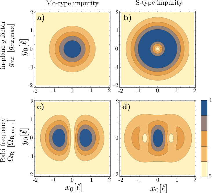
Clearly, the dependencies of and on are qualitatively different, which is illustrated in Fig. 3a and b. Both plots show circular symmetry: the results depend only on the length of but not on its direction, see Eq. (22) and (26). In case of the Mo-type impurity, Fig. 3a, the in-plane -factor decreases monotonically as is increased, following the Gaussian probability density of the envelope function at the position of the impurity. However, the in-plane factor due to an S-type impurity, Fig. 3b, is different, it is zero if the impurity is at the QD center, and reaches its maximal value if the impurity is at a distance from the QD center.
These results imply that in principle, the in-plane -factor in a MoS2 QD with a short-range impurity can be tuned electrically, by reshaping or replacing the QD as the voltages on the confinement gates are changed. For example, in the presence of an S-type impurity, the impurity-induced intervalley coupling, and thereby the corresponding decoherence processes, could be suppressed by electrostatically tuning the QD to , i.e., without spatially separating the impurity and the electron. Also, the dependence of the in-plane factor on the impurity position is qualitatively different for Mo-type and S-type impurities. This implies that experiments, where, e.g., magneto-transport spectroscopy maps the factor as a function of QD shape and location, could reveal information about the type, number, and position of the impurities in the QD.
VI Electrically driven qubit Rabi oscillations
Here we show that the spin-valley qubit defined in the MoS2 QD can be coherently controlled by an ac electric field, if a tilted magnetic field is applied, and at least one short-range impurity is present in the dot. In this case, the ac electric field induces qubit Rabi oscillations, when the qubit evolves coherently and cyclically between the two basis states and , if the driving frequency is chosen to be resonant with the qubit’s Larmor frequency . Our goal is to calculate the Rabi frequency characterizing these oscillations.
Similarly to the preceding section, here we also map our Hamiltonian , acting in an infinite-dimensional Hilbert space, to a two-dimensional effective qubit Hamiltonian. Note that in this case, is time dependent due to the presence of the ac electric field in . We use time-dependent Schrieffer-Wolff perturbation theory[50], treating as the perturbation, to obtain the qubit Hamiltonian. We find that the leading-order time-dependent term in the effective qubit Hamiltonian appears in the 3rd order of perturbation theory, and reads
| (29) |
where
| (30) |
This coupling appears due to the interplay of the in-plane magnetic field, the ac electric field and the impurity. Fig. 2b illustrates one of the three-step paths via virtual intermediate states that contribute to this coupling. Note that the fact that the only intervalley impurity matrix element appearing in Eq. (29) is is due to the choice that the driving electric field is along the direction and that the confinement potential is parabolic.
We consider the magnetic-field hierarchy , for which the qubit Larmor frequency is dominated by the out-of-plane component of the magnetic field. In this case, the qubit Larmor frequency is given by . We want to describe the electrically induced dynamics of this qubit with the initial state being . Upon resonant or almost-resonant driving, , and assuming that the driving is weak, the dynamics remains in the two-dimensional space of the spin-valley qubit, and the qubit will show simple Rabi oscillations, characterized by the Rabi frequency given by Eq. (30).
From Eqs. (30), the Rabi frequency is proportional to the impurity matrix element , which can be calculated for a Mo-type impurity using Eq. (14). We find that the dependence of the Rabi frequency as a function of the impurity position is given by
| (31) |
where the maximal value of the Rabi frequency is
| (32) |
The dependence of the Rabi frequency Eq. (31) on the impurity position is shown in Fig. 3c. The key features are: (i) The Rabi frequency is maximized when the position of the impurity is . (ii) The Rabi frequency decreases when the impurity is moved outside from the QD. (iii) The Rabi frequency is exactly zero if the impurity is placed in the QD center, or on the line .
Feature (iii) can be explained as follows. The external ac electric field along the axis induces a spatial oscillation of the electron in the direction, therefore the relative position of the impurity and the QD also oscillates with a small amplitude. Since, as seen in Fig. 3a, the in-plane factor depends on the relative position according to the spatial oscillation of the wave function leads to a temporal oscillation of , driving a Rabi oscillation between spin-valley qubit basis states. However, in the vicinity of the line , depends on quadratically, therefore the ac electric field does not generate a time-dependent in first order, and therefore the Rabi frequency is zero.
If the impurity in the QD is S-type, then the Rabi frequency is expressed from Eqs. (30), (16), (25), and
| (33) |
as
| (34) |
where
| (35) |
The spatial dependence of the Rabi frequency is plotted in Fig. 3d; the main features are as follows. (i) the Rabi frequency reaches its maximal value if the impurity is in the centre of the QD. (ii) There is no coherent transition if the impurity is placed at the position . (iii) The Rabi frequency has a local maximum if the monovacancy is at the position . We note that the simple explanation of the previous paragraph, applied for the Mo-type impurity and based on the adiabatic modulation of the in-plane -factor, does not explain features (i) and (iii) in the case of an S-type impurity. We anticipate that in this case, the relation between the -factor and the qubit dynamics can be characterized by a combination of the ‘Zeeman-modulation’ and ‘iso-Zeeman-modulation’ mechanisms[51].
VII Quantifying the results for MoS2
In this work, the in-plane -factor and the electrically driven Rabi oscillations are described in the perturbative regime, see Eq. (17), where the spin-orbit splitting is a large energy scale. In this regime, the coupling between the spin-valley qubit basis states decreases as the spin-orbit splitting is increased. Among the semiconductor ML-TMD materials, MoS2 has the smallest spin-orbit splitting[35]. Therefore, this seems to be the material best suited to observe the effects predicted here. Here we quantify the in-plane -factor and Rabi frequency for a single-electron spin-valley qubit in a ML MoS2 QD.
We consider a QD with orbital level spacing meV. Using , the oscillator length is nm. According to numerical studies of ML MoS2, the spin-orbit gap is meV and the valley factor is [35]. We assume a magnetic field with in-plane component T, and a driving electric field with amplitude kV/m. The latter value implies that the amplitude of the electron’s spatial oscillations is 6 nm, smaller than the oscillator length , so the perturbative treatment described above is justified.
If the Mo-type impurity is a Mo vacancy, and it is placed at the QD center, then Eq. (22) combined with the numerical estimate[41] gives meV for the intervalley impurity matrix element. This value is larger than the orbital level spacing, in disagreement with the assumption Eq. (17). Therefore, our results (23) and (31) for the -factor and Rabi frequency can be applied for a Mo vacancy in MoS2 only if the distance of the vacancy from the QD centre is larger than 32 nm; in this case the orbital level spacing exceeds the impurity matrix element, and hence a perturbative treatment of the latter is valid. Of course, our results (23) and (31) can also be applied for other Mo-type defects in MoS2 or in other ML-TMDC materials, if the corresponding impurity matrix elements are below the orbital level spacing.
If the S-type impurity is a S vacancy, then the maximal value of intervalley impurity matrix element according to Eq. (26) is 0.8 eV, complying with the perturbative hierarcy of Eq. (17). Then, the value of the maximal in-plane factor Eq. (28) is , and the maximal Rabi-frequency from Eq. (35) is MHz. Note that in this example, also the intravalley QD impurity matrix element is smaller then the orbital level spacing, and therefore using the harmonic-oscillator envelope functions as the orbital basis is a reasonable approximation. (Based on the numerical results of Ref. 41, we estimate , implying eV for the parameter set considered here.)
VIII Conclusions
In this work, we have proposed and analysed a way to coherently control a single-electron spin-valley qubit, that is defined in a QD in a ML-TMDC material, e.g., MoS2. Qubit control is performed in a fashion similar to electrically driven spin resonance: a resonant ac electric field drives Rabi oscillations with the help of an in-plane magnetic field and a short-range impurity; the former flips the spin and the latter flips the valley. For the case of a S-type impurity in the QD, we estimated that electrically driven qubit Rabi frequencies of the order of 10-100 MHz can be achieved. We also revealed and discussed the unconventional dependence of the in-plane factor and the electrically driven Rabi frequency on the impurity position, which arises for S-type impurities due to symmetry-forbidden intervalley scattering. Our results provide design guidelines for efficient electric control of spin-valley qubits in monolayer MoS2, which are promising building blocks for quantum information processing experiments, expected to show boosted coherence times, especially in isotopically purified samples.
IX Acknowledgments
We acknowledge useful discussions with G. Burkard, R. Frisenda, K. Kaasbjerg, J. Pető, and L. Tapasztó. GSz and AP acknowledge the financial support of the National Research, Development and Innovation Office of Hungary via the National Quantum Technologies Program NKP-2017-00001 and the OTKA Grants 105149, 108676 and 124723. LC acknowledges funding from the European Union’s Seventh Framework Programme (FP7/2007-2013) through the ERC Advanced Grant NOVGRAPHENE (GA No. 290846) and the Comunidad de Madrid through the grant MAD2D-CM, S2013/MIT-3007. AP is supported by the ÚNKP-17-4-III New National Excellence Program of the Ministry of Human Capacities of Hungary.
Appendix A Notation and preliminaries: perturbation theory
Here, we review the elements of theory that are relevant for the description of conduction-band electrons in the ML-TMDC materials studied here. These considerations are required to describe intervalley scattering by S-type impurities, e.g., an S vacancy in MoS2.
The single-electron Hamiltonian of the perfect crystal is
| (36) |
where the crystal potential is denoted by with . The eigenstates of are Bloch states:
| (37) |
where is the band index, is the sample area, and the lattice-periodic functions are normalized as
| (38) |
The corresponding eigenvalues (i.e., the band structure) are denoted as .
Our quantum dot holds a single conduction electron in a spatially slowly varying confinement potential. In this setup, the electronic wave function can be described via Bloch states from the vicinity of the conduction-band edge, that is, from the vicinity of the and points of the Brillouin zone. For crystal momenta around, e.g., , we can use first-order perturbation theory to express the conduction-band () Bloch states with the band-edge Bloch states – this procedure is called perturbation theory. In this theory, the so-called Kohn-Luttinger basis functions are used to form a matrix representation of the Hamiltonian:
| (39) | |||||
In the Kohn-Luttinger basis, the crystal Hamiltonian reads
| (40) |
where , the fully diagonal kinetic energy term was omitted, and
| (41) |
with .
The next step in theory is to reduce the multi-band problem defined by the crystal Hamiltonian to the conduction band. For this, second-order Schrieffer-Wolff perturbation theory[49] can be applied, where the fully diagonal first term of Eq. (40) is the unperturbed Hamiltonian, and the second () term of Eq. (40) forms the perturbation. The Schrieffer-Wolff transformation has the form , where the expression for the anti-Hermitian first-order transformation matrix is[49]
| (42) |
and the resulting effective conduction-band Hamiltonian reads
| (43) |
Here, we introduced the inverse effective mass tensor via
| (44) |
where is the dyadic product. Note that since a threefold rotation around an out-of-plane axis is a symmetry of the lattice, the effective mass is isotropic, i.e., this tensor is diagonal.
The effective conduction-band Hamiltonian matrix is diagonal, so its eigenvectors can be labelled by the wave vector , and have the trivial structure . The corresponding eigenvalue is . To obtain the corresponding Bloch state , we have to invert the Schrieffer-Wolff transformation,
Making a linear expansion of the exponential, and using the the first-order result (42) for the transformation matrix, we obtain the perturbative first-order approximation for the Bloch state as
| (46) | |||||
| (47) |
where the arguments are suppressed. This result is used in this work to evaluate the linear-in-momentum component of the intervalley matrix elements of a short-range impurity. Note that this treatment, i.e., taking into account the -induced hybridisation of the conduction band with remote bands, is required only for S-type impurities, where a linear-in- expansion of the intervalley matrix element is needed to obtain a nonzero result.
Appendix B S-type impurity: symmetry constraints of the bulk intervalley matrix element
For an S-type impurity, the symmetries of the conduction-band-edge Bloch function and the atomic structure pose the constraint (15) on the linear-in- contribution of the bulk intervalley impurity matrix element , defined in Eq. (13). Here we derive this constraint, with the specification that the Bloch states in the definition (13) are given by the result (47).
The generic expression for the linear-in- bulk intervalley impurity matrix element, without any symmetry restrictions, is
| (48) |
where the 5 coefficients are complex numbers. It is natural to expect that the rotational symmetry () provides a relation between and , and that time-reversal symmetry provides a relation between and . We derive these relations here, transform them to relations between the 5 coefficients, and thereby simplify the general expression in Eq. (48).
To exploit the rotational symmetry , we start from
| (49) |
On the one hand, from Eq. (47), we know
and that this is a non-degenerate Bloch state with energy eigenvalue . On the other hand, we know[36, 41] how the band-edge Bloch states transform under rotation around an S site: with and , and in particular. Combining these with Eq. (47), we find
Importantly, this is also a Bloch state with energy . Since the Bloch states (B) and (B) have the same energy and momentum, they must be identical, up to a complex phase factor. This requirement implies
| (52) |
We describe the -valley Bloch states as time-reversed -valley Bloch states, , yielding , and
| (53) |
Combining Eqs. (52) and (53) in Eq. (49), and exploiting the rotational symmetry of the impurity potential, results in
| (54) |
To exploit time reversal symmetry , which is the complex conjugation in our case, fulfilling , we start from
| (55) |
Again, we describe the -valley Bloch states as time-reversed -valley Bloch states: . Using this together with the time-reversal symmetry of the impurity potential, i.e., that the latter is real-valued, we find
| (56) |
The symmetry-based equations (54) and (55) must hold for any values of the wave-vector components , , , . Therefore, these equations form a set of 10 complex linear equations for the 5 complex unknown coefficients. We solve this linear set, and apply the resulting relations in Eq. (48), yielding
| (57) |
Clearly, inherits a global complex phase factor from the band-edge Bloch state , and hence with appropriate choice of global complex phase for we can make positive. Hence, we have proven that the form of the bulk intervalley impurity matrix elements follow Eq. (15), with the identification .
Note that the key difference between the Mo-type and S-type impurities is the transformation factor . I.e., both types of impurities preserve the rotation around the impurity site as a symmetry of the structure. However, the rotation around the Mo-type impurity transforms[41] the conduction-band-edge state as , that is, with , implying that is finite in general for a Mo-type impurity, and therefore can be used to approximate the intervalley impurity matrix elements between the QD wave functions.
Appendix C Quantum-dot wave functions from the envelope-function approximation
We have described the wave function of the electron in our QD via Eq. (3), i.e., as a wave packet, formed by the conduction-band Bloch states expressed from theory. Here we summarize how Eq. (3) is obtained from the envelope-function approximation (EFA).
The Hamiltonian of the electron in the QD is the sum of the crystal Hamiltonian and the QD confinement potential . The EFA is an extension of theory: it also relies on the Kohn-Luttinger matrix representation of the Hamiltonian, which is now given by Eq. (40) plus . Exploiting the spatially slowly varying nature of and the orthogonality of the functions of different bands, the interband matrix elements are neglected, . Furthermore, intervalley matrix elements of are neglected. This approximation is justified by the numerical results of Ref. 36, which imply that in our example, the order of magnitude of the confinement-induced intervalley matrix element does exceed 1 neV, it remains well below the impurity-induced intervalley matrix element of a single S vacancy (, see our Section VII).
Similarly to theory, the next step in the EFA is to reduce the multi-band problem of to the conduction band via the Schrieffer-Wolff transformation, treating the confinement potential as part of the perturbation. Importantly, since the interband matrix elements of the confinement potential are neglected, the interband perturbation remains the same as in the absence of the confinement potential, which implies that the Schrieffer-Wolff transformation matrix has exactly the same form as in theory, i.e., Eq. (42). The transformation results in the following effective conduction-band Hamiltonian (cf. Eq. (43)):
| (58) |
Recall that the effective mass tensor is isotropic; this fact was used in Eqs. (1) and (2).
Solutions of the matrix Schrödinger equation
| (59) |
are usually derived by Fourier transforming this equation to a real-space envelope-function Schrödinger equation, yielding Eq. (2), finding the solution of the latter, and Fourier transforming the envelope function to momentum space, yielding the coefficients .
To express the real-space wave function corresponding to the eigenvector of the transformed Hamiltonian , we have to invert the Schrieffer-Wolff transformation [cf. Eq. (A)]:
| (60) |
Using a linear expansion of the Schrieffer-Wolff transformation matrix in the perturbation, we obtain
| (61) |
which is then utilized in the main text as Eq. (3). In words, Eq. (61) expresses the fact that each electronic real-space energy eigenfunction of the QD is a packet of Bloch waves from the vicinity of the point, and the coefficients of this wave packet can be obtained from the envelope-function Schrödinger equation.
Appendix D The complete third-order qubit Hamiltonian
In the main text, we have presented the effective spin-valley qubit Hamiltonian that is required to describe the in-plane factor and the electrically driven Rabi oscillations. For completeness, here we present the third-order effective Hamiltonian, including the third-order time-independent term that was not discussed in the main text.
Recall that performing a second-order (time-independent) Schrieffer-Wolff transformation yields as shown by Eqs. (18), (19), and (20). Performing a third-order time-dependent Schrieffer-Wolff transformation[50] we find
| (62) |
where the first- and second-order terms are the same as above, the time-dependent third-order term is given in Eq. (29), and the time-independent third-order term is
| (63) | |||||
As in the main text, , , are Pauli matrices acting on the perturbed states and , see Sec. IV. The three subsequent terms describe the nonlinear Zeeman effect, and a higher-order correction of the out-of-plane and in-plane -factors, respectively.
References
- [1] R. Hanson, L. P. Kouwenhoven, J. R. Petta, S. Tarucha, and L. M. K. Vandersypen, Rev. Mod. Phys. 79, 1217 (2007).
- [2] J. R. Petta, A. C. Johnson, J. M. Taylor, E. A. Laird, A. Yacoby, M. D. Lukin, C. M. Marcus, M. P. Hanson, and A. C. Gossard, Science 309, 2180 (2005).
- [3] C. Flindt, A. S. Sørensen, and K. Flensberg, Phys. Rev. Lett. 97, 240501 (2006).
- [4] V. N. Golovach, M. Borhani, and D. Loss, Phys. Rev. B 74, 165319 (2006).
- [5] E. I. Rashba, Phys. Rev. B 78, 195302 (2008).
- [6] K. C. Nowack, F. H. L. Koppens, Y. V. Nazarov, and L. M. K. Vandersypen, Science 318, 1430 (2007).
- [7] S. Nadj-Perge, S. M. Frolov, E. P. A. M. Bakkers, and L. P. Kouwenhoven, Nature 468, 1084 (2010).
- [8] S. Nadj-Perge, V. S. Pribiag, J. W. G. van den Berg, K. Zuo, S. R. Plissard, E. P. A. M. Bakkers, S. M. Frolov, and L. P. Kouwenhoven, Phys. Rev. Lett. 108, 166801 (2012).
- [9] C. E. Nebel, Nat. Mater. 12, 690 (2013).
- [10] R. Maurand, X. Jehl, D. Kotekar-Patil, A. Corna, H. Bohuslavskyi, R. Laviéville, L. Hutin, S. Barraud, M. Vinet, M. Sanquer, and S. De Franceschi, Nat. Comm. 7, 13575 (2016).
- [11] F. A. Zwanenburg, A. S. Dzurak, A. Morello, M. Y. Simmons, L. C. L. Hollenberg, G. Klimeck, S. Rogge, S. N. Coppersmith, and M. A. Eriksson, Rev. Mod. Phys. 85, 961 (2013).
- [12] D. Culcer, A. L. Saraiva, B. Koiller, X. Hu, and S. Das Sarma, Phys. Rev. Lett. 108, 126804 (2012).
- [13] N. Rohling and G. Burkard, New Journal of Physics 14, 083008 (2012).
- [14] E. A. Laird, F. Pei, and L. P. Kouwenhoven, Nat. Nanotech. 8, 565 (2013).
- [15] A. Pályi and G. Burkard, Phys. Rev. Lett. 106, 086801 (2011).
- [16] A. Pályi and G. Burkard, Phys. Rev. B 82, 155424 (2010).
- [17] Y. Li, S. C. Benjamin, G. A. D. Briggs, and E. A. Laird, Phys. Rev. B 90, 195440 (2014).
- [18] K. Flensberg and C. M. Marcus, Phys. Rev. B 81, 195418 (2010).
- [19] K. S. Novoselov, A. Mishchenko, A. Carvalho, and A. H. Castro Neto, Science 353, 6298 (2016).
- [20] R. Roldan, L. Chirolli, E. Prada, J. A. Silva-Guillen, P. San-Jose, and F. Guinea, Chem. Soc. Rev. 46, 4387 (2017).
- [21] I. Žutić, J. Fabian, and S. Das Sarma, Rev. Mod. Phys. 76, 323 (2004).
- [22] W. Han, APL Materials 4, 032401 (2016).
- [23] J. R. Schaibley, H. Yu, G. Clark, P. Rivera, J. S. Ross, K. L. Seyler, W. Yao, and X. Xu, Nat. Rev. Materials 1, 16055 (2016).
- [24] Q. H. Wang, K. Kalantar-Zadeh, A. Kis, J. N. Coleman, and M. S. Strano, Nat Nano 7, 699 (2012).
- [25] E. Cappelluti, R. Roldán, J. A. Silva-Guillén, P. Ordejón, and F. Guinea, Phys. Rev. B 88, 075409 (2013).
- [26] R. Roldán, M. P. López-Sancho, F. Guinea, E. Cappelluti, J. A. Silva-Guillén, and P. Ordejón, 2D Materials 1, 034003 (2014).
- [27] A. Kormányos, V. Zólyomi, N. D. Drummond, P. Rakyta, G. Burkard, and V. I. Fal’ko, Phys. Rev. B 88, 045416 (2013).
- [28] X.-X. Song, D. Liu, V. Mosallanejad, J. You, T.-Y. Han, D.-T. Chen, H.-O. Li, G. Cao, M. Xiao, G.-C. Guo, and G.-P. Guo, Nanoscale 7, 16867 (2015a).
- [29] G. Luo, Z.-Z. Zhang, H.-O. Li, X.-X. Song, G.-W. Deng, G. Cao, M. Xiao, and G.-P. Guo, Frontiers of Physics 12, 128502 (2017).
- [30] X.-X. Song, Z.-Z. Zhang, J. You, D. Liu, H.-O. Li, G. Cao, M. Xiao, and G.-P. Guo, Scientific Reports 5, 16113 EP (2015b).
- [31] M. Javaid, D. W. Drumm, S. P. Russo, and A. D. Greentree, Nanotechnology 28, 125203 (2017).
- [32] K. Wang, T. Taniguchi, K. Watanabe, and P. Kim, “Engineering quantum confinement in semiconducting van der waals heterostructure,” ArXiv:1610.02929 (unpublished).
- [33] Z.-Z. Zhang, X.-X. Song, G. Luo, G.-W. Deng, V. Mosallanejad, T. Taniguchi, K. Watanabe, H.-O. Li, G. Cao, G.-C. Guo, F. Nori, and G.-P. Guo, Sci. Adv. 3, 1701699 (2017).
- [34] J. Klinovaja and D. Loss, Phys. Rev. B 88, 075404 (2013).
- [35] A. Kormányos, V. Zólyomi, N. D. Drummond, and G. Burkard, Phys. Rev. X 4, 011034 (2014).
- [36] G.-B. Liu, H. Pang, Y. Yao, and W. Yao, New Journal of Physics 16, 105011 (2014).
- [37] Y. Wu, Q. Tong, G.-B. Liu, H. Yu, and W. Yao, Phys. Rev. B 93, 045313 (2016).
- [38] A. J. Pearce and G. Burkard, 2D Materials 4, 025114 (2017).
- [39] M. Brooks and G. Burkard, Phys. Rev. B 95, 245411 (2017).
- [40] K. M. Itoh and H. Watanabe, MRS Communications 4, 143 (2014).
- [41] K. Kaasbjerg, T. Low, and A.-P. Jauho, ArXiv e-prints (2016), arXiv:1612.00469 [cond-mat.mes-hall] .
- [42] K. Kaasbjerg, J. H. J. Martiny, T. Low, and A.-P. Jauho, Phys. Rev. B 96, 241411 (2017).
- [43] J. Hong, Z. Hu, M. Probert, K. Li, D. Lv, X. Yang, L. Gu, N. Mao, Q. Feng, L. Xie, J. Zhang, D. Wu, Z. Zhang, C. Jin, W. Ji, X. Zhang, J. Yuan, and Z. Zhang, Nat Commun 6, 6293 (2015).
- [44] W. Zhou, X. Zou, S. Najmaei, Z. Liu, Y. Shi, J. Kong, J. Lou, P. M. Ajayan, B. I. Yakobson, and J.-C. Idrobo, Nano Letters 13, 2615 (2013).
- [45] Y.-C. Lin, T. Björkman, H.-P. Komsa, P.-Y. Teng, C.-H. Yeh, F.-S. Huang, K.-H. Lin, J. Jadczak, Y.-S. Huang, P.-W. Chiu, A. V. Krasheninnikov, and K. Suenaga, Nature Communications 6, 6736 (2015).
- [46] P. Vancsó, G. Z. Magda, J. Pető, J.-Y. Noh, Y.-S. Kim, C. Hwang, L. Biró, and L. Tapasztó, Sci. Rep. 6, 29726 (2016).
- [47] A. Pályi and G. Burkard, Phys. Rev. B 80, 201404 (2009).
- [48] G. Széchenyi and A. Pályi, Phys. Rev. B 89, 115409 (2014).
- [49] R. Winkler, Spin-Orbit Coupling Effects in Two-Dimensional Electron and Hole Systems (Springer-Verlag, 2003).
- [50] J. Romhányi, G. Burkard, and A. Pályi, Phys. Rev. B 92, 054422 (2015).
- [51] A. Crippa, R. Maurand, L. Bourdet, D. Kotekar-Patil, A. Amisse, X. Jehl, M. Sanquer, R. Laviéville, H. Bohuslavskyi, L. Hutin, S. Barraud, M. Vinet, Y.-M. Niquet, and S. D. Franceschi, “Electrical spin driving by g-matrix modulation in spin-orbit qubits,” ArXiv:1710.08690 (unpublished).