Design of graph filters and filterbanks
Abstract
Basic operations in graph signal processing consist in processing signals indexed on graphs either by filtering them, to extract specific part out of them, or by changing their domain of representation, using some transformation or dictionary more adapted to represent the information contained in them. The aim of this chapter is to review general concepts for the introduction of filters and representations of graph signals. We first begin by recalling the general framework to achieve that, which put the emphasis on introducing some spectral domain that is relevant for graph signals to define a Graph Fourier Transform. We show how to introduce a notion of frequency analysis for graph signals by looking at their variations. Then, we move to the introduction of graph filters, that are defined like the classical equivalent for 1D signals or 2D images, as linear systems which operate on each frequency of a signal. Some examples of filters and of their implementations are given. Finally, as alternate representations of graph signals, we focus on multiscale transforms that are defined from filters. Continuous multiscale transforms such as spectral wavelets on graphs are reviewed, as well as the versatile approaches of filterbanks on graphs. Several variants of graph filterbanks are discussed, for structured as well as arbitrary graphs, with a focus on the central point of the choice of the decimation or aggregation operators.
1Graph Fourier Transform and Frequencies
1.1Introduction
Graph Signal Processing (GSP) has been introduced in the recent past using at least two complementary formalisms: on the one hand, the discrete signal processing on graphs [1] which emphasizes the adjacency matrix as a shift operator on graph and develops an equivalent of Discrete Signal Processing (DSP) for signals on graphs; and on the other hand, the approaches rooted in graph spectral analysis, which rely on the spectral properties of a Laplacian matrix (or operator) on a graph [2, 3, 4]. Both approaches yield an analogy for harmonic analysis of graph signals through the definition of a Graph Fourier Transform as being the projection of a signal in the spectral domain of the chosen matrix or operator. While the technical details vary, and some interpretations in the vertex domain may differ, the fundamental objective of both approaches is to decompose a signal onto components of different frequencies and to design filters that can extract or modify parts of a graph signal according to these frequencies, e.g. providing notions of low-pass, band-pass, or high-pass filters for graph signals. In this section, both approaches (along with other variations) are seen as specific instances of the general guideline for defining Graph Fourier Transform and its associated frequency analysis.
Notations.
Vectors are written in bold with small letters, and matrices in bold and capital letters. Let be a graph with the set of nodes, the set of edges, and the weighted adjacency matrix in . If , there is no connection from node to node , otherwise, is the weight of the edge starting from and pointing to 11 1 In the literature, the converse convention is sometimes chosen (e.g. in [1]), hence the occasionally appearing in this chapter.. If an undirected edge exists between and , then . We restrict ourselves to adjacency matrices with positive or null entries: . Finally, the symbol denotes the identity matrix (its dimension should be clear with the context), and is a vector whose -th entry is equal to while all other entries are equal to .
1.2Graph Fourier Transform
Definition 1.1 (graph signal).
A graph signal is a vector whose component is considered to be defined on vertex .
A Graph Fourier Transform (GFT) is defined via a choice of reference operator admitting a spectral decomposition. Representing a graph signal in this spectral domain is interpreted as a GFT. We review the standard properties and the various definitions proposed in the literature.
Consider a matrix . To be admissible as a reference operator for the graph, it is often required that for any pair of nodes , and are equal to zero if and are not connected, as this will help for efficient implementations of filters (see in 2.4). We assume furthermore that is diagonalizable in . In fact, if is not diagonalizable, one needs to consider Jordan’s decomposition, which is out-of-scope of this chapter. We refer the reader to [1] for technical details on how to handle this case. Nevertheless, in practice, we claim that it often suffices to consider only diagonalizable operators, since: i) diagonalizable matrices in are dense in the space of matrices; and ii) graphs under consideration are generally measured (should they model social, sensor or biological networks,…) with some inherent noise. So, if one ends up unluckily with a non-diagonalizable matrix, a small perturbation within the noise level will make it diagonalizable – provided the graphs have no specific regularities that are to be kept. Still, we may assume with only a small loss of generality that the reference operator has a spectral decomposition:
| (1) |
with and in . The columns of , denoted , are the right eigenvectors of , while the lines of , denoted , are its left eigenvectors. is the diagonal matrix of the eigenvalues . The GFT is defined as the transformation of a graph signal from the canonical “node” basis to its representation in the eigenvector basis:
Definition 1.2 (Graph Fourier Transform).
For a given diagonalizable reference operator acting on a graph , the GFT of a graph signal is:
| (2) |
The GFT’s coefficients are simply the projections on the left eigenvectors of :
| (3) |
Moreover, the GFT is invertible: . While, in general, the complex Fourier modes are not orthogonal to each other, when is symmetric, the following additional properties hold true.
The special case of symmetric reference operators. If in addition to be real, is also symmetric, then and are real matrices, and may be found orthonormal, that is: . In this case, , the GFT of is simply
with coefficients , and the Parseval relation holds: . Hereafter, when a symmetric operator is encountered, one should have these properties in mind.
Finally, the interpretation of the graph Fourier modes in terms of oscillations and frequencies will be the scope of Section 1.3. In the following, we list possible choices of reference operators, all diagonalizable with different and , thus all defining different possible GFTs.
GFT for undirected graphs
Undirected graphs are characterized by symmetric adjacency matrices: . This does not necessarily mean that has to be chosen symmetric as well, as we will see with the example below.
The following choices of are the most common in the undirected case.
The combinatorial Laplacian [symmetric].
The first choice for , advocated in [2, 3, 4] is to
use the graph’s combinatorial Laplacian, having properties studied in [5]. It is defined as
where is the diagonal matrix of nodes’ strengths, defined as .
If the adjacency matrix is binary (i.e., unweighted), this strength reduces to the degree of each node.
The advantages of using are twofold.
i) It is an intuitive manner to define the GFT: being the discretized version of the continuous Laplacian operator which admits the Fourier modes as eigenmodes, it is fair to use by analogy the eigenvectors of as graph Fourier modes. Moreover, this choice is associated to a complete theory of vector calculus (e.g., gradients) for graph signals [6] that is useful to solve PDE’s on graphs. ii) has well known mathematical properties [5], giving
ways to characterize the graph or functions and processes on the graph (see also [7]).
Most prominently, it is semi-definite positive (SDP) and its eigenvalues, being all positive or null, will
serve in the following to bind eigenvectors with a notion of frequency.
The normalized Laplacian [symmetric]. A second choice for is the normalized Laplacian
. An interesting property of this choice of Laplacian is that all its eigenvalues lie between 0 and 2 [5].
The adjacency matrix, or deformed Laplacian [symmetric]. Another choice for is the adjacency matrix22
2
We use instead of for consistency purposes with [1], whose convention for directed edges in the adjacency matrix is converse to ours: what they call is what we call . Without any influence in the undirected case, it has an impact in the directed case. , as advocated in [1]. One readily sees that the eigenbasis of and the eigenbasis of the deformed Laplacian , where is the operator 2-norm, are the same. Therefore, the corresponding GFTs are equivalent and, for consistency in the presentation, we will use here.
The random walk Laplacian [not symmetric]. The random walk Laplacian is yet another Laplacian reading: , where
serves also to describe a uniform random walk on the graph.
Even though is not symmetric, we know it diagonalizes in . In fact, if is an eigenvector of with eigenvalue , then is an eigenvector of with same eigenvalue. Thus, has the same eigenvalues as , and its Fourier basis is real but not orthonormal.
Other possible definitions of the reference operator. For instance, the consensus operator (of the form with some suitable ) [8],
a geometric Laplacian [9], or some other deformed Laplacian one may think of, are valid alternatives.
All these operators imply a different spectral domain (different and ) and, provided one has a nice frequency interpretation (which is the object of Section 1.3), they all define possible GFTs. In the graph signal processing literature, the first three operators (, and ) are the most widely used.
GFT for directed graphs
For directed graphs, the adjacency matrix is no longer symmetric – is not necessarily equal to – which does not automatically imply that the reference operator is not symmetric (e.g., the case below). This case is of great interest in some applications where the graph is naturally directed such as hyperlink graphs (there is a directed edge between website and website if there is a hyperlink in website directing to ). In directed graphs, the degree of node is separated in its out-degree, , and its in-degree, .
Some straightforward approaches [not symmetric]. It is possible to readily transpose the previous notions to the directed case, choosing either or to replace in the different formulations: e.g. as in [10], as in [11],
.
A notable choice is to directly use as in [1] (we recall that and are equivalent for they share the same eigenvectors and thus, define the same GFT).
These matrices are no longer strictly speaking Laplacians as they are no longer SDP, but one may nonetheless consider them as reference operators defining possible GFTs. Note that these definitions entail to choose (rather arbitrarily) either or in their formulations, with the notable exception of . In fact, naturally generalizes to the directed case and is a classical choice of in this context [1].
Chung’s directed Laplacian [symmetric]. A less common approach in the graph signal processing community is the one provided by the directed Laplacians introduced by Chung [12]. To define these Laplacians appropriate to the directed case, let us first introduce the random walk transition matrix (or operator) defined as . It admits a stationary probability33 3 Assuming the random walk is ergodic, i.e. irreducible and non-periodic. such that . Writing , Chung defines the following two directed Laplacians:
| (4) | ||||
| (5) |
Both the combinatorial and the normalized directed Laplacians verify the properties of Laplacian matrices:
SDP, negative (or null) entries everywhere except on the diagonal and real symmetric.
It is easy to see that (4) and (5) generalise the definitions of the undirected case since for an undirected graph,
, ; hence is the combinatorial Laplacian , and is its normalized version .
Other possible definitions of the reference operator. The previous definitions of and for undirected graphs may also be generalized to the directed Laplacian framework to obtain:
| (6) |
Additional notes. Other GFTs for directed graphs were proposed via the Hermitian Laplacian as introduced in [13], which generalizes . A very different approach is to construct a Graph Fourier basis directly from an optimization scheme, requiring some notion of smoothness, or generalization of it – see [14, 15]. We will not consider this recent approach here.
1.3Frequencies of graph signals
To complement the notion of GFT, one needs to introduce some frequency analysis of the Fourier modes on the graph. The general way of doing so is to compute how fast a mode oscillates on the graph, and the tool of preference is to compute their variations along the graph. Let us first note the following facts:
- •
In the undirected case, is semi-definite positive (SDP). In fact, one may write:
(7) This function is also called the Dirichlet form. Similarly, is also SDP:
(8) As far as we know, the Dirichlet forms of and do not have such a nice formulation as a sum of local quadratic variations over all edges of the graph. They are nevertheless SDP because: i) and have the same spectrum; ii) the symmetry of implies real eigenvalues, and the maximum eigenvalue of being by definition of the norm, the minimum eigenvalue of is 0.
- •
In the directed case, all directed Laplacians , , and are SDP due to similar arguments. and also have Dirichlet forms in terms of a sum of local quadratic variations, e.g.:
(9) The other reference operators , , , are not SDP as their eigenvalues may be complex. Nevertheless, the real part of their eigenvalues are always non-negative. This is quite clear for . For , as the sum of row of is equal to , Gershgorin circle theorem ensures that all eigenvalues of are non-negative. For , as is a stochastic matrix, the Perron-Frobenius theorem ensures that its eigenvalues are in the disk of radius 1 in the complex plane, hence the real part of ’s eigenvalues are non-negative. As and have the same set of eigenvalues, it is also true for .
To sum up, all the reference operators considered are either SDP (with real non-negative eigenvalues) or have eigenvalues whose real component is non-negative.
Definition 1.3 (Graph frequency).
Let be a reference operator. If its eigenvalues are real, the generalized graph frequency of a graph Fourier mode is:
| (10) |
If its eigenvalues are complex, two different definitions of the generalized graph frequency of a graph Fourier mode exist:
| (11) |
Remarks. In the complex eigenvalues case, it is a matter of choice wether we consider the imaginary part of the eigenvalues or not. There is no current consensus on this question. Also, note that all eigenvectors associated to the same have the same frequency. We thus define the frequency of an eigenspace, denoted by .
Justification: the link between frequency and variation. Two types of variation measures have been considered in the literature to show the consistency between this definition of graph frequencies and a notion of oscillation over the graph. The first one is based on the quadratic forms of the Laplacian operators. For instance, in the undirected case with the combinatorial Laplacian, Eq. (7) applied to any normalized Fourier mode defined from reads:
| (12) |
The larger the local quadratic variations of , the larger its frequency . Eqs. (8) and (9) (as well as its counterpart for ) enable to make this variation-frequency link for and . The second general type of variation that has been defined [16] is the total variation between a signal and its shifted version on the graph (where “shifting” a signal is understood as applying the adjacency matrix to it). For instance, in the case of , the associated variation reads44 4 In [16], the norm is used, but the norm can be used equivalently: this is a matter of how one wants to normalize the eigenvectors. In this paper, we consider the classical Euclidean norm, hence .:
| (13) |
where designate the eigenvalues of and the one of maximum magnitude. The variation of the graph Fourier mode from thus reads:
| (14) |
The larger the total variation of , that is, the further is from its shifted version along the graph, the larger its frequency55 5 There is a direct correspondence between , the eigenvalues of , and : . We thus recover the results in [16]: the closer is from in the complex plane, the smaller the total variation of the associated Fourier mode .. For , a similar approach detailed in [10] links the variation of to its frequency .
It may also happen that for some operator , none of these two types of variations (quadratic forms or total variation) show natural. Then, one may use the variation based on another related operator to define frequencies. For instance, in [11, 17], authors considered the random walk Laplacians as the reference operator to define the GFT, while the directed combinatorial Laplacian is used to measure the variations. With these choices, they showed that is equal to up to a normalization constant. Another example of such a case is in [18] where one of the reference operators to build filters is the isometric translation introduced in [19] while the variational operators are built upon the combinatorial Laplacian. Note finally that other notions of variations like the Hub authority score can be drawn from the literature. We refer the reader to [20] for details on that, as well as a complementary discussion on GFTs and their related variations.
Definition 1.3 associates graph frequencies only to graph Fourier modes. For an arbitrary signal, we have the following definition of its frequency analysis:
Definition 1.4 (Frequency analysis).
The frequency analysis of any graph-signal on is given by its components at frequency , as given in Definition 1.3.
a)  b)
b) 
c)
d)
1.4Implementation and illustration
Implementation. The implementation of the GFT requires to diagonalize , costing operations in general, and memory space to store . Then, applying to a signal to obtain costs operations. These costs are prohibitive for large graphs ( nodes). Recent works investigate how to reduce these costs, by tolerating an approximation on . In the cases where is symmetric, authors in [22, 23] suggest to approximate by a product of Givens rotations, using a truncated Jacobi algorithm. The resulting approximated fast GFT requires operations to compute the Givens rotations, and operations to compute the approximate GFT of . The difficulty in designing fast GFTs boils down to the difficulty of deciphering eigenvalues that are very close to one another. This difficulty disappears once we consider smooth filtering operations that are much easier to efficiently approximate, as we will see in the next section.
Illustrations. To illustrate the GFT and the notion of frequency, we show in Fig. 1 two graph signals on the Karate club graph [21], corresponding to instances of a low frequency and a high frequency signal, respectively. We also show their GFTs, computed for three different choices of : , and .
The choice of normalization and the choice to take explicitly the degree matrix into account or not in the definition of has a quantitative impact on the GFTs. Nevertheless, qualitatively, a graph signal that varies slowly (resp. rapidly) along any path of the graph is low-frequency (resp. high-frequency). In Fig. 2, we show how the GFT is not only sensitive to the graph signal but also to the underlying graph structure.
a) 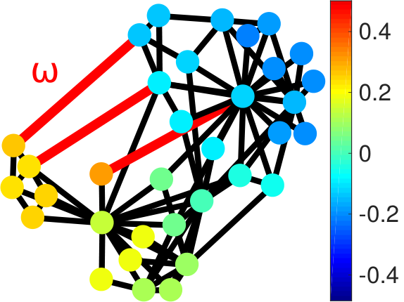 b)
b)
2Graph filters
In this section, we assume that the reference operator of the graph on which we wish to design filters is diagonalizable in as in the previous section. The order of the eigenvalues and eigenvectors is chosen frequency-increasing. That is, given a choice of frequency definition (either or ), one has .
2.1Definition of graph filters
The reference operator has an eigendecomposition as in Eq. (1), and it can also be written as a sum of projectors on all its eigenspaces:
| (15) |
where the sum is on all different eigenvalues and is the projector on the eigenspace associated to eigenvalue , i.e.:
Definition 2.1 (wide-sense definition of a graph filter).
The most general definition of a graph filter is an operator that acts separately on all the eigenspaces of , depending on their eigenvalue . Mathematically, any function
| (16) | ||||
| (17) |
defines a graph filter such that
| (18) |
The decomposition of the filter on each eigenspace of with eigenvalue is associated to a filtering weight that attenuates or increases the importance of this eigenspace in the decomposition of the signal of interest. In fact, one may write the action of on a graph signal as:
| (19) |
For any function , let us write as a shorthand notation for . A graph filter can be written as:
| (20) |
Using functional calculus of operators, this is equivalently written as , which calls for some interpretation remarks. In fact, this expression opens the way to interpret what is the action of a graph filter in the vertex domain. Firstly, note that applying to a graph signal is in fact a local computation on the graph: on each node, the resulting transformed signal is a weighted sum of the values of the original signal on its (direct) neighbours. Therefore, in the node space, a filter can be interpreted as an operator that weights the information on the signal transmitted through edges of the graph, the same way classical filters are built on the basic operation of time-shift. This fundamental analogy shift/reference operator was first made in [1] with the adjacency matrix and was particularly pertinent in that case. Yet, in the GSP literature, some authors extended this analogy to all reference operators, using sometimes the generic term “graph shift operators” for their designation.
Now, to illustrate the notion of graph filtering in the spectral domain, consider the graph signal and . The -th Fourier component of being, by construction, , its filtered version reads:
| (21) |
Hence the -th Fourier component of the filtered signal is , recalling the classical interpretation of filtering as a multiplication in the Fourier domain. We call the frequency response of the filter.
In many cases, it is more convenient and natural to restrict ourselves to functions that associate the same real number to all values of . That is, considering any two eigenvalues and associated to the same frequency , we restrict ourselves to functions such that . This entails the following narrowed-sense definition of a graph filter.
Definition 2.2 (narrowed-sense definition of a graph filter).
Any function
| (22) | ||||
| (23) |
defines a narrowed-sense graph filter such that
| (24) |
Examples of narrowed-sense filters:
- •
The constant filter equal to : . In this case, and : all frequencies are allowed to pass, and no component is filtered out.
- •
The Kronecker delta in : . If there exists one (or several) eigenvalues of such that , then . If not, then . For this filter, only the frequency is allowed to pass.
- •
The ideal low-pass with cut-off frequency : if , and otherwise. In this case: , i.e., only frequencies up to are allowed to pass.
- •
The heat kernel : the weight associated to is exponentially decreasing with the frequency . Actually is the solution of the graph diffusion (or heat) equation (see [2]) at time with initial condition .
2.2Properties of graph filters
From now on, in order to simplify notations and concepts in this introductory chapter on graph filtering, we will restrict ourselves to symmetric reference operators, such as , , or in the undirected case, or the directed Laplacians or in the directed case. In this case, the eigenvalues are real such that the frequency definition is straightforward , both filter definitions are equivalent such that the frequency response reads
| (25) | ||||
| (26) |
and one may find a real orthonormal graph Fourier basis such that . A filtering operator associated to thereby reads:
| (27) |
All results presented in the following may be (carefully) generalized to the unsymmetric case.
Definition 2.3.
We write the set of finite-order polynomials in :
| (28) |
Proposition 2.1.
is equal to the set of graph filters.
Proof.
Consider . Then, defining , one has: , i.e., is a filter. Now, consider a filter, i.e., there exists such that . Consider the polynomial that interpolates through all pairs . The maximum degree of such a polynomial is as there are maximum points to interpolate, and may be smaller if eigenvalues have multiplicity larger than one. Thereby, one may write: . Writing , this means that . ∎
Consequence: An equivalent definition of a graph filter is a polynomial in of maximal degree .
Definition 2.4.
We write the set of all diagonal operators in the graph Fourier space:
| (29) |
Proposition 2.2.
The set of graph filters is included in . Both sets are equal iff all eigenspaces of are of dimension one (i.e., all eigenvalues are of multiplicity one).
Proof.
By definition of graph filters, they are included in . Now, in general, an element of is not necessarily a graph filter. In fact, given , all diagonal entries of may be chosen independently, which is not the case for the diagonal entries of corresponding to the same eigenspace. Thus, both sets are equal iff all eigenspaces are of dimension one. ∎
Consequence: In the case where all eigenvalues are simple, an equivalent definition of a graph filter is a diagonal matrix in the graph Fourier basis.
Definition 2.5.
We write the set of matrices that commute with :
| (30) |
Proposition 2.3.
. The equality holds iff all eigenvalues of are simple.
Proof.
A polynomial in necessarily commutes with , thus . Now, in general, an element in is not necessarily in . In fact, if , then with . Suppose . In this case, commutativity does not constrain at all, thereby is not necessarily in . Now, if we suppose that all eigenvalues have multiplicity one, i.e., all diagonal entries of are different, the only solution for is to be a diagonal matrix, i.e., . We showed in Prop. 2.2 that the set of graph filters is equal to iff all eigenvalues have multiplicity one, therefore: iff all eigenvalues have multiplicity one. ∎
Consequence: In the case where all eigenvalues are simple, an equivalent definition of a graph filter is a linear operator that commutes with .
2.3Some designs of graph filters
From the previous sections, it should now be clear that the frequency response of a filter only alters the frequencies corresponding to the discrete set of eigenvalues of (see Eq. (18)). More generally though, the frequency response of a graph filter can be defined over a continuous range of ’s, leading to the notion of universal filter design, i.e. a filter whose frequency response is designed for all ’s and not only adapted to the specific eigenvalues of . On the contrary, a graph-dependent filter design depends specifically on these eigenvalues.
FIR filters. From the results of Section 2.2, a natural class of graph filters is given in the form of Finite Impulse Response (FIR) filters, as by eq. (28) with a polynomial of finite order, which realizes a weighted Moving Average (MA) filtering of a signal. Also, one can design any universal filter by fitting the desired response with a polynomial . The larger is, the closer the filter can approximate the desired shape. If the approximation is done only using the , the design is graph-dependent, else it is universal if fitting some function function .
Let us then go back to the interpretation of as a graph shift operator in the node space and see how it operates for FIR filters. Applied to a graph signal, the terms in eq. (28), act as a -hops local computation on the graph: on each node, the resulting filtered signal is a weighted sum of the values of the original signal lying in its -th neighbourhood, that is, nodes attainable with a path of length along the graph. Then, like for classical signals, FIR filters only imply a finite neighbourhood of each nodes, and this will translate in Section 2.4 into distributed, fast implementations of these filters. Still, FIR filters are usually poor at approximating filters with sharp changes of desired frequency response, as illustrated for instance in Fig. 1 of [24].
ARMA filters. A more accurate and approximation of can be obtained with a rational design [24, 25, 26]:
| (31) |
Such a rational filter is called an Auto-Regressive Moving Average filter of order and is commonly noted ARMA. Again, it is known from classical DSP that an ARMA design, being a IIR (Infinite Impulse Response) filter, is more versatile at approximating various shapes of filters, especially with sharp changes in the frequency response. The filtering relation for ARMA filters can be written in the node domain as: . This ARMA filter expression will lead to the distributed implementation, discussed later in 2.4. For instance, for an ARMA(1,0) (i.e., an AR(1)) one will have to use: .
Example: A first design of low-pass graph filtering is given by the simplest least-square denoising problem, where the the Dirichlet form is used as Tikhonov regularization promoting smoothness on the graph. Using the (undirected) Laplacian and assuming one observes , the filter is given by;
| (32) |
The solution is then given in the spectral domain (for ) by with . It turns out to be a (universal) AR(1) filter.
Design of coefficients. To design the coefficients of ARMA filters, the classical approach is to find the set of coefficients and to approximate the desired as a rational function. However, as recalled in [24, 25], the usual design in DSP are not easily transposed to the GSP framework because the frequency response is given in terms of the ’s, and not in terms of or .
Henceforth, it has been studied in [24, 25] how to approximate the filter coefficients in a universal manner (i.e., with no specific reference to the graph spectrum) using a Shank’s method: 1) Determine the by first finding a polynomial approximation of , and solve the system of equations to identify the ’s. Then 2) solve the least-square problem to minimize w.r.t. to find the ’s.
A second method is to approximate the filter response in a graph-dependent design, on the specific frequencies only. To do so, the method in [27], instead of fitting the polynomial ratio, solves the following optimization problem:
| (33) |
Using again a polynomial approximation , the solution derives from the least square solution (see details in [27]).
AR filters to model random processes. We do not discuss much in this chapter random processes on graphs ; for that see the framework to study stationary random processes on graphs in [28, 29]. Still, a remark can be done for the parametric modeling of random processes. As introduced in [1], one can model a process on a graph as the output of a graph filter, generally taken as an ARMA filter. Here, we discuss the case of AR filters. The linear prediction is written as:
| (34) |
The coefficients of this filter can directly be obtained by numerical inversion of where . The solution is given by the pseudo-inverse: which minimizes the squared error , w.r.t to . Another possibility would be to estimate the coefficients of the AR model by means of the orthogonality principle leading to the Yule-Walker (YW) equations, as follows:
| (35) |
Depending to the structure of the reference operator , we have:
- 1)
If is symmetric (, as often for undirected graph), the autocorrelation function involved in this YW system is: ;
- 2)
When is unitary (for instance with as the isometric operator from [19]), the corresponding autocorrelation will be and the usual techniques to solve the YW system can be used.
Experimentally, it was found that the isometric operator of [19] or a consensus operator are the one that offer a more exact and stable modeling [18].
2.4Implementations of graph filters
Given a frequency response , how to effectively implement the action of the corresponding graph filter on a graph signal ?
The direct approach. It consists in first diagonalizing to obtain and ; then computing the filter matrix ; before finally left-multiplying the graph signal by to obtain its filtered version. The overall computational cost of this procedure is arithmetic operations due to the diagonalization and memory space as the graph Fourier transform is in general dense.
The polynomial approximate filtering approach. More efficiently though, we can first, quickly estimate and (for instance via the power method) and second, look for a polynomial that best approximates on the whole interval . Let us call the coefficients of this approximate polynomial. We have:
| (36) |
The number of required arithmetic operations is , where is a trade-off between precision and computational cost. Also, the easier is approachable by a low-order polynomial, the better the approximation. At the same time, the larger is, the more accurate the approximation is. The authors of [30] recommend as a natural choice for the approximation polynomials, the Chebychev polynomials as they are known to be optimal in the -norm sense.
In some circumstances, other choices can be preferred. For instance, when approximating the ideal low-pass, Chebychev polynomials yield Gibbs oscillations around the cut-off frequency that turn penalising for smooth filters. In that case, other choices are possible [31], such as the Jackson-Chebychev polynomials that attenuate such unwanted oscillations.
The Lanczos approximate filtering approach. In [32], and based on works by [33], authors propose an approximate filtering approach based on Lanczos iterations. Given a signal , the Lanczos algorithm computes an orthonormal basis of the Krylov subspace associated to : , as well as a small tridiagonal matrix such that: . The approximate filtering then reads:
| (37) |
At fixed , this approach has a typical complexity in , possibly raised to if a reorthonomalisation is needed to stabilize the algorithm;
a cost that is comparable to that of the polynomial approximation approach.
Theoretically, the quality of approximation is similar (see [32] for details). In practice however, it has been observed that if the spectrum is regularly spaced, polynomial approximations should be prefered, while the Lanczos method has an edge over others in the case of irregularly-spaced spectra. This is understandable as Krylov subspaces are also used for diagonalisation purposes (see for instance, chapter 6 of [34]) and thus naturally adapt to the underlying spectrum.

Distributed implementation of ARMA filters. The ARMA filters being defined through a rational fraction, are IIR filters. Henceforth, the polynomials approach to distribute and fasten the computation are not the most efficient ones. The methods developed in [25, 26] yield a distributed implementation of ARMA filters. The first point is to remember that the rational filter off eq. (31) can be implemented from its partial fraction decomposition as a sum of polynomial fractions of order 1 only. Then, the distributed implementation of filtering can be done by studying the 1st order recursion [25]:
| (38) |
where is the filter output at iteration . The operator M is chosen equal to , with the same eigenvectors as , and with a minimal spectral radius that ensures good convergence properties for the recursion. The coefficient and are chosen in so that, with and , the proposed recursion reproduces the effect of the following ARMA(1,0) filter: . The coefficients and are the residue and the pole of the rational function, respectively.
Because M is local in the graph, the recursive application of eq. (38) is local and the algorithm is then naturally distributed on the graph, with a memory and operation at each recursion in for filters in parallel to compute the output of a ARMA filter.
This approach is shown in [25, 26] to converge efficiently. Moreover, in [24], the behavior of this design is also studied in time-varying settings, when the graph and the signal are possibly time-varying; it is then shown that the recursion can remain stable and usable as a distributed implementation of IIR filters.
3Filterbanks and multiscale transforms on graphs
To process and filter signals on graphs, it is attractive to develop equivalent of multiscale transforms such as wavelets, i.e. ways to decompose a graph signal on components at different scales, or frequency ranges. The road to multiscale transforms on graphs has originally been tackled in the vertex domain [35] to analyse data on networks. Thereafter, a general design of multiscale transforms was based on the diffusion of signals on the graph structure, leading to the powerful framework of Diffusion Wavelets [36, 37]. This latter works were already based on a diffusion operators, usually a Laplacian or a random walk operator, whose powers are decomposed in order to obtain a multiscale orthonormal basis. The objective was to build a kind of equivalent of discrete wavelet transforms for graph signals.
In this chapter, we focus on two other constructions of multiscale transforms on graphs which are more related to the Graph Fourier Transform. The frequency analysis and filters described here are: 1) the method of [3] which develops an analog of continuous wavelet transform on graphs, 2) approaches that combine filters on graphs with graph decompositions through decimation (pioneered in [4] with decimation of bipartite graphs) or aggregation of nodes; in a nutshell, these methods are very close to the filter banks implementation of discrete wavelets [38].
3.1Continuous multi-scale transforms
In the following, we work with undirected graphs and , whose eigenvalues are contained in the interval . The generalization to other operators can be done using the guidelines of previous sections.
The first continuous multiscale transform based on the graph Fourier transform was introduced via the spectral graph wavelet transform [3] (and inherent of some properties of the concept of diffusion polynomial frames [39]). These wavelets were defined by analogy to the classical wavelets in the following sense. Classically, a wavelet family centered around time and at scale is the translated and dilated version of a mother wavelet , generally defined as a zero-mean, square integrable function. Mathematically it is expressed for all and as:
| (39) |
or equivalently, in the frequency domain, with the continuous Fourier transform:
| (40) |
Then, for a signal , the wavelet coefficient at scale and instant is given by the inner product .
By analogy, transposing eq. (40) with GFT, a spectral graph wavelet at scale and node reads66 6 Note that the scale parameter stays continuous, but the localization parameter is discretized to the set of nodes of the graph.:
| (41) |
where the graph filter plays the role of the wavelet bandpass filter . The shifted scaled wavelet identifies to the impulse response of to a Dirac localized on node . In particular, the shape of the filter originally proposed in [3] was:
with , , and four parameters, and the unique cubic polynomial interpolation that preserves continuity and the derivative’s continuity. Several properties on the obtained wavelets may be theoretically derived, for instance the notion of locality (the fact that wavelets’ energy is mostly contained around the node on which it is centered). Given a selection of scales and a graph signal , the signal wavelet coefficient associated to the node and the scale reads: . Then, a question that naturally arises is that of invertibility of the wavelet transform: can one recover any signal from its wavelet coefficients? As defined here, the wavelet transform is not invertible as it does not take into account –due to the zero-mean constraint of the wavelets– the signal’s information associated to the null frequency, i.e., associated to the first eigenvector . To enable invertibility, one may simply add any low-pass filter to the set of filters of the wavelet transform. We write their associated atoms:
| (42) |
The following theorem derives:
Theorem 3.1 (Theorem 5.6 in [3]).
Given a set of scales , the set of atoms forms a frame with bounds , given by:
| (43) | ||||
| (44) |
where .
In theory, invertibility is guaranteed provided that is different from 0. Nevertheless, in practice, one should strive to design filter shapes (wavelet and low-pass filters) and to choose a set of scales such that is as close as possible to in order to deal with well-conditioned inverses. Doing so, we obtain the so-called tight (or snug) frames, i.e. frames such that (or ). An approach is to use classical dyadic decompositions using bandlimited filters such as in Table 1 of [40]. Another desirable property of such frames is their discriminatory power: the ability at discerning different signals only by considering their wavelet coefficients. For a filterbank to be discriminative, each filter element needs to take into account information from a similar number of eigenvalues of the Laplacian. The eigenvalues of an arbitrary graph being unevenly spaced on , one needs to compute or estimate the exact density of the spectrum of the graph under consideration [41].
3.2Discrete multi-scale transforms
A second general way to generate multiscale transforms is via a succession of filtering and decimation operations, as in Fig. 4. This scheme is usually cascaded as in 5, and each level of the cascade represents a scale of description of the input signal. Thereby, as soon as decimation enters into the process, we talk about “discrete” multi-scale transforms, as the scale parameter can no longer be continuously varied. For details on this particular approach to multiscale transforms in classical signal processing, we refer e.g. to the book by Strang and Nguyen [38]. In the following, we directly consider the graph-based context. Let us first settle notations:
- •
The decimation operator may be generally defined by partitioning the set of nodes into two sets and . As this subdivision is a partition, we have and . Moreover, let us define the downsampling operator associated to : given any graph signal , is the reduction of to . We also define the upsampling operator . Given a signal defined on , is the zero-padded version of on the whole graph. The combination of both operators reads: , where is the indicator function of . Moreover, we define
(45) - •
We define and respectively a low-pass and a high-pass graph filter, called analysis filters. and are also two graph filters, called synthesis filters. All filters are associated to their frequency responses , , and .
The signal is called the approximation of , whereas is generally understood as the necessary details to recover from its approximation.
Given the scheme of Fig. 4, one writes the processed signal as:
| (46) | ||||
| (47) |
When designing such discrete filterbanks, and in order to enable perfect reconstruction (), one deals with two main equations linking all four filters and the matrix :
| (48) | |||
| (49) |
Left-multiplying by and right-multiplying by , one obtains equivalently:
| (50) | |||
| (51) |
Eq.(50) is purely spectral, and may be seen as a set of equations:
| (52) |
On the other hand, Eq. (51) is not so simple due to the decimation operation and needs to be investigated in detail.
In 1D classical signal processing (equivalent to the undirected circle graph), the decimation operator samples one every two nodes. Moreover, given , one classically has the following aliasing phenomenon (Theorem 3.3 of [38]):
| (53) |
This means that the decimation operations may be explictly described in the Fourier space, which greatly simplifies calculations by enabling to write Eq. (51) as a purely spectral equation as well. Moreover, this also entails that the combined filtering-decimation operations may be understood as a global multiscale filter (yet with discrete scales), thereby connecting with the previous approach. Now, the central question that remains is how to mimick the filtering/decimation approach on general graphs?
In Section 3.2.1, it will be shown that for very well structured graphs such as bipartite graphs or -cyclic graphs, generalizations of the decimation operator may be defined and their effect explicitly described as graph filters. Then the case of arbitrary graph is studied in 3.2.2 where the “one every two nodes” paradigm is not transposable directly; several approaches to do that will then be reviewed.
3.2.1Filterbanks on bipartite graphs and other strongly structured graphs
Filterbanks on bipartite graphs. Bipartite graphs are graphs where the nodes are partitioned in two sets of nodes and such that all links of the graph connect a node in with a node in . On bipartite graphs, the “one-every-two-node” paradigm has a natural extension: decimation ensembles are set to and . Leveraging the fact that bipartite graphs’ spectra are symmetrical77 7 i.e., if is an eigenvalue of , then so is around the value 1, Narang and Ortega [4] show the bipartite graph spectral folding phenomenon:
| (54) |
(with as in eq. 15). This means that for any filter one has:
| (55) |
Eq. (51) therefore boils down to a second set of purely spectral equations:
| (56) |
Eqs. (52) and (56) give us equations linking the parameters of the four filters to ensure perfect reconstruction. The other degrees of liberty are free to be used to design filterbanks with other desirable properties of filterbanks, such as (bi-)orthogonality, compact-supportness of the atoms, and of course also to adapt to the specific application for which these filters are designed.
Filterbanks on other regular structures. Extending these ideas, several authors have proposed similar approaches to define filterbanks on other regular structures such as -block cyclic graphs [42] or circulant graphs [43, 44]. In any case, writing decimation operations exactly as graph filters requires regular structures on graphs inducing at least some regularity in the spectrum one may take advantage of. All these approaches lead to exact reconstruction procedures. However, arbitrary graphs do not have such regularities, and other approaches are required.
3.2.2Filterbanks on arbitrary graphs
To extend the filterbanks approach to arbitrary graphs, one needs to either generalize the decimation operators, or to bypass it by working with operator of aggregation of nodes. We discuss in this last part some solutions that were proposed in the literature. A complementary and thoughtful discussion on graph decimation, graph aggregation and graph reconstruction can be found in sections III and IV of [45]. For that, the two key questions are:
- •
how to generalize the decimation operator on arbitrary graphs? We will see that generalized decimation operators either try to mimick the classical decimation and attempt to sample “one every two nodes”, or aggregate nodes to form supernodes according in general to some graph cut objective function.
- •
how to build the new coarser-scale graph from the decimated nodes (or aggregated supernodes)? In fact, after each decimation, if one wants to cascade the filterbank, a new coarse-grain graph has to be built in order to define the next level’s graph filters. The nodes (resp. supernodes) are set thanks to decimation (resp. aggregation): but how do we link them together?
Graph decimation. The first work to generalize filterbanks on arbitrary graphs is due to Narang and Ortega [4] and consists in decomposing the graph into an edge-disjoint collection of bipartite subgraphs, and then to apply the scheme presented in Section 3.2.1 on each of the subgraphs. In this collection, each subgraph has the same node set, and the union of all subgraphs sums to the original graph. To perform this decomposition (which is not unique), the same authors propose a coloring-based algorithm, called Harary’s decomposition. Sakiyama and Tanaka [46] also used this decomposition as one of their design’s cornerstone. Unsatisfied by the NP-completeness of the coloring problem (even though heuristics exist), Nguyen and Do [47] propose another decomposition method based on maximum spanning trees.
The bipartite paradigm’s main advantage comes from the fact that decimation has an explicit formulation in the graph’s Fourier space, thereby enabling exact filter designs depending on the given task. In our opinion, when applied to arbitrary graphs, its main drawback comes from the non-unicity of the bipartite subgraphs decomposition, as well as the seamingly arbitrariness of such a decomposition: from a graph signal point-of-view, what is the meaning of a bipartite decomposition? Letting go of this paradigm, and slightly changing the general filterbank design presented in Section 3.2.1, other generalized graph decimations have been proposed. For instance, in [48], authors propose to separate the graph in two sets according to its max cut, i.e., maximizing . In [45], authors suggest similarly to partition the graph into two sets according to the polarity of the last eigenvector (i.e. the eigenvector associated to the highest frequency). In [49], authors use an original approach based on random forests to sample nodes, where they have a probabilistic version of “equally-spaced” nodes on the graph.
Graph aggregation. Another paradigm in graph reduction is graph aggregation, where, instead of selecting nodes as in decimation, aggregates entire regions of the graph in “supernodes”. In general, these methods are based on first clustering the nodes in a partition . Each of these subsets will define a supernode of the coarse graph: this reduced graph thus contains supernodes. Once a rule is chosen to connect these supernodes together (the object of the next paragraph), the coarse graph is fully defined, and the method may be iterated to obtain a multiresolution of the initial graph’s structure. All these methods differ mainly on the choice of the algorithm or the objective function to find this partition. For instance, one may find methods based on random walks [50], on short time diffusion distances [51], on the algebraic distance [52], etc. Other multiresolution approaches may also be found in [53, 54, 55]. One may also find many approaches from the network science community in the connex field of community detection [56, 57], and in particular multiscale community detection [58, 59, 60]. All these methods are concerned about providing a multiresolution description of the graph structure, but do not consider any graph signal. Recently, graph signal processing filterbanks have been proposed to define a multiscale representation of graph signals based on these approaches. In [61], we proposed such an approach where we define a generalized Haar filterbank: instead of averaging and differentiating over pairs of nodes as in the classical Haar filterbank, we average and differentiate over the subsets of a partition in subgraphs. In [62], authors propose a similar approach and define other types of filterbanks such as the hierarchical graph Laplacian eigentransform. Another similar Haar filterbank may be found in [37]. All these methods are independent of exactly which aggregation algorithm one chooses to find the partition. Let us also cite methods that provide multiresolution approaches without necessarily defining low-pass and high-pass filters explictly in the graph Fourier domain [63, 37, 64]. Finally, let us point out that these methods may be extended to graph partitions containing overlaps, as in [65].
Coarse graph reconstruction. Once one decided how to decimate nodes, or how to partition them in supernodes, how should one connect these nodes together in order to form a consistent reduced graph?
In order to satisfy constraints such as interlacement (coarsely speaking, that the spectrum of the reduced graph is representative of the spectrum of the initial graph) and sparsity, Shuman et al. [45] propose a Kron reduction followed by a sparsification step. The Laplacian of the reduced graph is thus defined as the Schur complement of the initial graph’s Laplacian relative to the unsampled nodes. The sparsification step is performed via a sparsifier based on effective resistances by Spielman and Srivastava [66] that approximately preserves the spectrum. In [49], authors propose another approach to the intuitive idea that the initial and coarse graph should have similar spectral properties: they look for the coarse Laplacian matrix that satisfies an intertwining relation. In [47], authors connect nodes according to the set of nested bipartite graphs obtained by their maximum spanning tree algorithm. In aggregation methods [61, 62], there is an inherent natural way of connecting supernodes: the weight of the link between supernodes and is equal to the sum of the weights of the links connecting nodes in to nodes in .
Illustrations. We show in Fig. 6 an example of multiresolution analysis of a given graph signal on the Minnesota traffic graph, using a method of successive graph aggregation to compute the details and approximations at different scales. The specific method for this illustration is the one detailed in [61].

Conclusion
The purpose of this chapter was to introduce the reader to a basic understanding of what is a Graph Fourier Transform. We stressed how it can be generally introduced for undirected or directed graphs, by choosing a reference operator whose spectral domain will define the frequency domain for graph signals. Then, we led the reader to the more elaborated designs of graph filters and multiscale transforms on graphs. The first section is voluntarily introductory, and almost self-contained. Indeed, we endeavoured to delineate a general guideline that shows, in an original manner, that there is no major discrepancy between choosing a Laplacian, an Adjacency, or a random walk operator…as long as one chooses accordingly, the appropriate notion of frequency to analyse graph signals. Then, after a proper definition of graph filters, our objective was to review the literature and to propose guidelines and pointers to the relevant results on graph filters and related multiscale transforms. This last part being written as a review, we beg for reader’s indulgence, as many details are skipped, and some works are only reported here in a sketchy manner.
Acknowledgements
This work was supported by the ANR grant Graphsip ANR-14-CE27-0001-02 and ANR-14-CE27-0001-03.
References
- [1] A. Sandryhaila and J. Moura, “Discrete signal processing on graphs,” Signal Processing, IEEE Transactions on, vol. 61, no. 7, pp. 1644–1656, April 2013.
- [2] D. Shuman, S. Narang, P. Frossard, A. Ortega, and P. Vandergheynst, “The emerging field of signal processing on graphs: Extending high-dimensional data analysis to networks and other irregular domains,” Signal Processing Magazine, IEEE, vol. 30, no. 3, pp. 83–98, May 2013.
- [3] D. Hammond, P. Vandergheynst, and R. Gribonval, “Wavelets on graphs via spectral graph theory,” Applied and Computational Harmonic Analysis, vol. 30, no. 2, pp. 129–150, 2011.
- [4] S. Narang and A. Ortega, “Perfect reconstruction two-channel wavelet filter banks for graph structured data,” Signal Processing, IEEE Transactions on, vol. 60, no. 6, pp. 2786–2799, June 2012.
- [5] F. Chung, Spectral graph theory. Amer Mathematical Society, 1997, no. 92.
- [6] L. Grady and J. R. Polimeni, Discrete Calculus: Applied Analysis on Graphs for Computational Science. Springer, 2010.
- [7] A. Barrat, M. Barthlemy, and A. Vespignani, Dynamical processes on complex networks. Cambridge University Press, 2008.
- [8] S. Kar and J. M. F. Moura, “Consensus + innovations distributed inference over networks: cooperation and sensing in networked systems,” IEEE Signal Processing Magazine, vol. 30, no. 3, pp. 99–109, May 2013.
- [9] H. Rabiei, F. Richard, O. Coulon, and J. Lefevre, “Local spectral analysis of the cerebral cortex: New gyrification indices,” IEEE Transactions on Medical Imaging, vol. 36, no. 3, pp. 838–848, March 2017.
- [10] R. Singh, A. Chakraborty, and B. S. Manoj, “Graph fourier transform based on directed laplacian,” in 2016 International Conference on Signal Processing and Communications (SPCOM), June 2016, pp. 1–5.
- [11] H. Sevi, G. Rilling, and P. Borgnat, “Multiresolution analysis of functions on directed networks,” in Wavelets and Sparsity XVII, Aug 2017.
- [12] F. Chung, “Laplacians and the Cheeger inequality for directed graphs,” Annals of Combinatorics, vol. 9, no. 1, pp. 1–19, 2005. [Online]. Available: http://link.springer.com/article/10.1007/s00026-005-0237-z
- [13] G. Yu and H. Qu, “Hermitian laplacian matrix and positive of mixed graphs,” Applied Mathematics and Computation, vol. 269, no. Supplement C, pp. 70 – 76, 2015. [Online]. Available: http://www.sciencedirect.com/science/article/pii/S0096300315009649
- [14] S. Sardellitti, S. Barbarossa, and P. D. Lorenzo, “On the graph fourier transform for directed graphs,” IEEE Journal of Selected Topics in Signal Processing, vol. 11, no. 6, pp. 796–811, Sept 2017.
- [15] R. Shafipour, A. Khodabakhsh, G. Mateos, , and E. Nikolova, “A digraph fourier transform with spread frequency components,” in Proc. of IEEE Global Conf. on Signal and Information Processing, Nov 2017.
- [16] A. Sandryhaila and J. Moura, “Discrete signal processing on graphs: Frequency analysis,” Signal Processing, IEEE Transactions on, vol. 62, no. 12, pp. 3042–3054, June 2014.
- [17] H. Sevi, G. Rilling, and P. Borgnat, “Analyse fréquentielle et filtrage sur graphes dirigés,” in 26e Colloque sur le Traitement du Signal et des Images. GRETSI-2017, Sept 2017, p. id. 220.
- [18] S. Ben Alaya, P. Gonçalves, and P. Borgnat, “Linear prediction on graphs based on autoregressive models,” in Graph Signal Processing Workshop, May 2016.
- [19] B. Girault, P. Goncalves, and E. Fleury, “Translation on graphs : An isometric shift operator,” Signal Processing Letters, IEEE, vol. 22, no. 12, Dec. 2015.
- [20] A. Anis, A. Gadde, and A. Ortega, “Efficient sampling set selection for bandlimited graph signals using graph spectral proxies,” IEEE Transactions on Signal Processing, vol. 64, no. 14, pp. 3775–3789, July 2016.
- [21] W. Zachary, “An information flow model for conflict and fission in small groups,” Journal of anthropological research, vol. 33, no. 4, pp. 452–473, 1977.
- [22] L. LeMagoarou, R. Gribonval, and N. Tremblay, “Approximate fast graph Fourier transforms via multi-layer sparse approximations,” IEEE Transactions on Signal and Information Processing over Networks, vol. PP, no. 99, pp. 1–1, 2017.
- [23] L. LeMagoarou, N. Tremblay, and R. Gribonval, “Analyzing the approximation error of the fast graph fourier transform,” in proceedings of the Asilomar Conference on Signals, Systems, and Computers, Nov 2017.
- [24] E. Isufi, A. Loukas, A. Simonetto, and G. Leus, “Autoregressive Moving Average Graph Filtering,” IEEE Transactions on Signal Processing, vol. 65, no. 2, pp. 274–288, Jan. 2017.
- [25] A. Loukas, A. Simonetto, and G. Leus, “Distributed autoregressive moving average graph filters,” IEEE Signal Processing Letters, vol. 22, no. 11, pp. 1931–1935, Nov 2015.
- [26] X. Shi, H. Feng, M. Zhai, T. Yang, and B. Hu, “Infinite Impulse Response Graph Filters in Wireless Sensor Networks,” Signal Processing Letters, IEEE, vol. 22, no. 8, pp. 1113–1117, 2015.
- [27] J. Liu, E. Isufi, and G. Leus, “Autoregressive moving average graph filter design,” in 6th Joint WIC/IEEE Symposium on Information Theory and Signal Processing in the Benelux, May 2016.
- [28] N. Perraudin and P. Vandergheynst, “Stationary signal processing on graphs,” IEEE Transactions on Signal Processing, vol. 65, no. 13, pp. 3462–3477, July 2017.
- [29] A. G. Marques, S. Segarra, G. Leus, and A. Ribeiro, “Stationary graph processes and spectral estimation,” IEEE Transactions on Signal Processing, vol. 65, no. 22, pp. 5911–5926, Nov 2017.
- [30] D. Shuman, P. Vandergheynst, and P. Frossard, “Chebyshev polynomial approximation for distributed signal processing,” in Distributed Computing in Sensor Systems and Workshops (DCOSS), 2011 International Conference on, June 2011, pp. 1–8.
- [31] N. Tremblay, G. Puy, R. Gribonval, and P. Vandergheynst, “Compressive spectral clustering,” in Proceedings of the 33 rd International Conference on Machine Learning (ICML), vol. 48. JMLR: W&CP, 2016, pp. 1002–1011. [Online]. Available: http://jmlr.csail.mit.edu/proceedings/papers/v48/tremblay16.pdf
- [32] A. Susnjara, N. Perraudin, D. Kressner, and P. Vandergheynst, “Accelerated filtering on graphs using Lanczos method,” arXiv preprint arXiv:1509.04537, 2015. [Online]. Available: https://arxiv.org/abs/1509.04537
- [33] E. Gallopoulos and Y. Saad, “Efficient Solution of Parabolic Equations by Krylov Approximation Methods,” SIAM Journal on Scientific and Statistical Computing, vol. 13, no. 5, pp. 1236–1264, 1992. [Online]. Available: https://doi.org/10.1137/0913071
- [34] Y. Saad, Numerical Methods for Large Eigenvalue Problems, 2nd ed., ser. Classics in Applied Mathematics 66. SIAM, 2011.
- [35] M. Crovella and E. Kolaczyk, “Graph wavelets for spatial traffic analysis,” in INFOCOM 2003. Twenty-Second Annual Joint Conference of the IEEE Computer and Communications. IEEE Societies, vol. 3, 2003, pp. 1848–1857.
- [36] R. Coifman and M. Maggioni, “Diffusion wavelets,” Applied and Computational Harmonic Analysis, vol. 21, no. 1, pp. 53–94, 2006.
- [37] M. Gavish, B. Nadler, and R. R. Coifman, “Multiscale wavelets on trees, graphs and high dimensional data: Theory and applications to semi supervised learning,” in Proceedings of the 27th International Conference on Machine Learning (ICML-10), 2010, pp. 367–374.
- [38] G. Strang and T. Nguyen, Wavelets and filter banks. SIAM, 1996.
- [39] M. Maggioni and H. Mhaskar, “Diffusion polynomial frames on metric measure spaces,” Applied and Computational Harmonic Analysis, vol. 24, no. 3, pp. 329–353, May 2008. [Online]. Available: http://linkinghub.elsevier.com/retrieve/pii/S106352030700070X
- [40] N. Leonardi and D. Van De Ville, “Tight wavelet frames on multislice graphs,” Signal Processing, IEEE Transactions on, vol. 61, no. 13, pp. 3357–3367, July 2013.
- [41] D. Shuman, C. Wiesmeyr, N. Holighaus, and P. Vandergheynst, “Spectrum-adapted tight graph wavelet and vertex-frequency frames,” Signal Processing, IEEE Transactions on, vol. PP, no. 99, pp. 1–1, 2015.
- [42] O. Teke and P. P. Vaidyanathan, “Extending Classical Multirate Signal Processing Theory to Graphs ; Part I: Fundamentals,” IEEE Transactions on Signal Processing, vol. 65, no. 2, pp. 409–422, Jan. 2017.
- [43] V. N. Ekambaram, G. C. Fanti, B. Ayazifar, and K. Ramchandran, “Circulant structures and graph signal processing,” in 2013 IEEE International Conference on Image Processing, Sep. 2013, pp. 834–838.
- [44] M. S. Kotzagiannidis and P. L. Dragotti, “Splines and wavelets on circulant graphs,” CoRR, vol. abs/1603.04917, 2016. [Online]. Available: http://arxiv.org/abs/1603.04917
- [45] D. I. Shuman, M. J. Faraji, and P. Vandergheynst, “A Multiscale Pyramid Transform for Graph Signals,” IEEE Transactions on Signal Processing, vol. 64, no. 8, pp. 2119–2134, Apr. 2016.
- [46] A. Sakiyama and Y. Tanaka, “Oversampled graph Laplacian matrix for graph filter banks,” Signal Processing, IEEE Transactions on, vol. 62, no. 24, pp. 6425–6437, Dec 2014.
- [47] H. Nguyen and M. Do, “Downsampling of signals on graphs via maximum spanning trees,” Signal Processing, IEEE Transactions on, vol. 63, no. 1, pp. 182–191, Jan 2015.
- [48] S. Narang and A. Ortega, “Local two-channel critically sampled filter-banks on graphs,” in Image Processing (ICIP), 2010 17th IEEE International Conference on, Sept 2010, pp. 333–336.
- [49] L. Avena, F. Castell, A. Gaudillière, and C. Mélot, “Intertwining wavelets or Multiresolution analysis on graphs through random forests,” 2017.
- [50] S. Lafon and A. B. Lee, “Diffusion maps and coarse-graining: a unified framework for dimensionality reduction, graph partitioning, and data set parameterization,” IEEE Transactions on Pattern Analysis and Machine Intelligence, vol. 28, no. 9, pp. 1393–1403, Sep. 2006.
- [51] O. E. Livne and A. Brandt, “Lean Algebraic Multigrid (LAMG): Fast Graph Laplacian Linear Solver,” SIAM Journal on Scientific Computing, vol. 34, no. 4, pp. B499–B522, 2012. [Online]. Available: https://doi.org/10.1137/110843563
- [52] D. Ron, I. Safro, and A. Brandt, “Relaxation-based coarsening and multiscale graph organization,” Multiscale Modeling & Simulation, vol. 9, no. 1, pp. 407–423, 2011. [Online]. Available: http://epubs.siam.org/doi/abs/10.1137/100791142
- [53] I. Dhillon, Y. Guan, and B. Kulis, “Weighted Graph Cuts without Eigenvectors A Multilevel Approach,” Pattern Analysis and Machine Intelligence, IEEE Transactions on, vol. 29, no. 11, pp. 1944–1957, Nov. 2007.
- [54] G. Karypis and V. Kumar, “A Fast and High Quality Multilevel Scheme for Partitioning Irregular Graphs,” SIAM Journal on Scientific Computing, vol. 20, no. 1, pp. 359–392, 1998. [Online]. Available: http://dx.doi.org/10.1137/S1064827595287997
- [55] F. Murtagh and P. Contreras, “Algorithms for hierarchical clustering: an overview,” Wiley Interdisciplinary Reviews: Data Mining and Knowledge Discovery, vol. 2, no. 1, pp. 86–97, 2012. [Online]. Available: http://dx.doi.org/10.1002/widm.53
- [56] M. E. Newman, “Modularity and community structure in networks,” Proceedings of the National Academy of Sciences, vol. 103, no. 23, pp. 8577–8582, 2006.
- [57] S. Fortunato, “Community detection in graphs,” Physics Reports, vol. 486, no. 3-5, pp. 75–174, 2010.
- [58] J. Reichardt and S. Bornholdt, “Statistical mechanics of community detection,” Phys. Rev. E, vol. 74, no. 1, p. 016110, Jul. 2006. [Online]. Available: http://link.aps.org/doi/10.1103/PhysRevE.74.016110
- [59] M. Schaub, J. Delvenne, S. Yaliraki, and M. Barahona, “Markov dynamics as a zooming lens for multiscale community detection: non clique-like communities and the field-of-view limit,” PloS one, vol. 7, no. 2, p. e32210, 2012.
- [60] N. Tremblay and P. Borgnat, “Graph Wavelets for Multiscale Community Mining,” Signal Processing, IEEE Transactions on, vol. 62, no. 20, pp. 5227–5239, Oct. 2014.
- [61] ——, “Subgraph-Based Filterbanks for Graph Signals,” IEEE Transactions on Signal Processing, vol. 64, no. 15, pp. 3827–3840, Aug. 2016.
- [62] J. Irion and N. Saito, “Applied and computational harmonic analysis on graphs and networks,” in Wavelets and Sparsity XVI, vol. 9597, Sep. 2015, pp. 95 971F–95 971F–15. [Online]. Available: http://dx.doi.org/10.1117/12.2186921
- [63] A. B. Lee, B. Nadler, and L. Wasserman, “Treelets: An Adaptive Multi-Scale Basis for Sparse Unordered Data,” The Annals of Applied Statistics, vol. 2, no. 2, pp. 435–471, 2008. [Online]. Available: http://www.jstor.org/stable/30244207
- [64] G. Mishne, R. Talmon, I. Cohen, R. R. Coifman, and Y. Kluger, “Data-Driven Tree Transforms and Metrics,” IEEE Transactions on Signal and Information Processing over Networks, vol. PP, no. 99, pp. 1–1, 2017.
- [65] A. D. Szlam, M. Maggioni, R. R. Coifman, and J. C. Bremer Jr, “Diffusion-driven multiscale analysis on manifolds and graphs: top-down and bottom-up constructions,” in Proc SPIE, vol. 5914, 2005, p. 59141D.
- [66] D. A. Spielman and N. Srivastava, “Graph Sparsification by Effective Resistances,” SIAM Journal on Computing, vol. 40, no. 6, pp. 1913–1926, 2011. [Online]. Available: http://dx.doi.org/10.1137/080734029