Hidden charm pentaquark and $\Lambda(1405)$ in the $\Lambda^{0}_{b}\to\eta_{c}K^{-}p(\pi\Sigma)$ reaction

The analysis of the $\Lambda^{0}_{b}\to J/\psi K^{-}p$ reaction of LHCb and the interpretation of the $J/\psi p$ spectrum in terms of the two pentaquark states, $P_{c}(4380)$ and $P_{c}(4450)$ [1, 2] has stirred a wave of theoretical work trying to understand the nature of the states. Prior to the experiment there were predictions based on molecular states of the $\bar{D}\Sigma_{c}-\bar{D}\Lambda_{c}$ and $\bar{D}^{*}\Sigma_{c}-\bar{D}^{*}\Lambda_{c}$ nature [3, 4]. These would be hidden charm molecular states, and in the case of $\bar{D}^{*}\Sigma_{c}-\bar{D}^{*}\Lambda_{c}$ a state with spin-parity $J^{P}=3/2^{-}$ appears with mass similar to the $P_{c}(4450)$. These two systems, studied within coupled channels, couple also to $\eta_{c}N$ in the first case and to $J/\psi N$ in the second one, the channel where the $P_{c}(4450)$ state was observed. The works of Refs. [3, 4] stimulated further research with this type of molecular states, studied with different dynamics in Refs. [5, 6, 7, 8, 9], or quark models [10], all them prior to the LHCb experiment. After the experimental observation many ideas have been proposed to interprete the nature of those pentaquark states. Molecular states coming from the interaction of meson-baryon have been suggested [11, 12, 13, 14, 15, 16, 17, 18, 19, 20, 21, 22, 23, 24, 25, 26, 27]. Pentaquark structures of type diquark-diquark-antiquark nature have also been proposed [28, 29]. Other different quark rearrangements have been suggested [30, 31, 32, 33], as well as QCD sum rules [34, 35], and new methods of production in different reactions have also been investigated [36, 37, 38, 39, 40, 41, 42, 43, 44]. The properties of these hidden charm states in light quark matter have also been studied in Ref. [45]. Reviews on the subject have also been written with detailed discussion of different works and ideas in Refs. [46, 47, 48, 49, 50, 51, 52, 53, 54, 55].

A suggestion to explain the $P_{c}(4450)$ peak as a manifestation of a triangle singularity [56, 57] was shown in Ref. [58] to be unable to explain the experimental feature with the preferred quantum numbers of the experiment $3/2^{-}$ or $5/2^{+}$.

Prior also to the experimental measurement of the $\Lambda^{0}_{b}\to J/\psi K^{-}p$ reaction [2, 1], a theoretical study was done in Ref. [59], where it was shown that the $K^{-}p$ was produced in isospin $I=0$ (as was later on corroborated by experiment) and also the invariant $K^{-}p$ mass distribution in $s$-wave (related to the $\Lambda(1405)$ production) and the invariant $\pi\Sigma$ mass distribution in the related $\Lambda^{0}_{b}\to J/\psi\pi\Sigma$ reaction, were studied.

The experimental analysis of the $\Lambda^{0}_{b}\to J/\psi K^{-}p$ reaction [2, 1] also showed the contribution of the $K^{-}p$ mass distribution from the $\Lambda(1405)$, which was in qualitative agreement with the one found in Ref. [59]. After the experiment was done, the consistency of the strength of the peak of the $P_{c}(4450)$ and the $K^{-}p$ strength coming from the $\Lambda(1405)$, were shown to be consistent with the findings of Refs. [3, 4] should the quantum number be $1/2^{-}$ [12], but this was generalized to other quantum numbers in Ref. [60]. Incidentally, in this latter work it was shown that, based on the $J/\psi p$ and $K^{-}p$ mass distributions alone, one could not determine the spin and parity of the states, nor the need for the wide $P_{c}(4380)$ state, which means that angular distributions and polarizations information must be the elements helping determining these quantum numbers in the experimental analysis.

In the present work we pay attention to the reaction of $\Lambda^{0}_{b}\to\eta_{c}K^{-}p$, which is under analysis by the LHCb collaboration [61] and make predictions for the $\eta_{c}p$ and $K^{-}p$ mass distributions. Simultaneously, we also study the $\Lambda^{0}_{b}\to\eta_{c}\pi\Sigma(\pi\Sigma\equiv\pi^{+}\Sigma^{-},\pi^{0}\Sigma^{0},\pi^{-}\Sigma^{+})$ reaction and make predictions for the $\pi\Sigma$ mass distribution which shows the $\Lambda(1405)$ shape. We use the predictions made for the $\bar{D}\Sigma_{c}-\bar{D}\Lambda_{c}$ and coupled channels in Refs. [3, 4] and can relate the $\pi\Sigma$ mass distribution with those of $\eta_{c}p$ and $K^{-}p$. The interesting thing is that a clear peak emerges in the $\eta_{c}p$ mass distribution due to a $1/2^{-}$ dynamically generated state, mostly for $\bar{D}\Sigma_{c}$, which couples relatively strongly to the $\eta_{c}p$ channel. The predictions done here should be of much use to guide experimental search and to get relevant conclusion from a comparison with experiment when this is finished.

This article is organized as follows. In Sec. II, we present the theoretical formalism of the decay of $\Lambda^{0}_{b}\to\eta_{c}K^{-}p$, explaining in detail the hadronization and final state interactions of the $\eta_{c}p$ and $K^{-}p$ pairs. Numerical results and discussions are presented in Sec. III, followed by a summary in the last section.

Following Ref. [59] we write the first step in the $\Lambda^{0}_{b}\to\eta_{c}K^{-}p$ reaction at the quark level, which proceeds as shown in Fig. 1. The $ud$ diquark in the $\Lambda^{0}_{b}$ is in $I=0$ and they are spectators in the decay. The final state $sud$ is again in $I=0$ and hence, only $\Lambda^{*}$ states should show up in the final state apart of the $c\bar{c}$ that now forms the $\eta_{c}$. Note that, apart from the $bcW$ coupling in the first weak vertex, the next coupling $csW$ is Cabibbo favored.

We must now proceed to produce $K^{-}p$ from the $sud$ cluster of the final state and we are interested in $K^{-}p$ in $s$-wave, which is what couples to the $\Lambda(1405)$, the dominant term close to the $K^{-}p$ threshold, as shown in the experimental analysis of the $\Lambda^{0}_{b}\to J/\psi K^{-}p$ reaction [2, 1]. Since $K^{-}p$ in $s$-wave has negative parity and the $u$, $d$ quarks are spectators, the $s$ quark must be produced in orbital angular momentum $L=1$ in the diagram of Fig. 1. Yet, since finally in $K^{-}p$ all quarks are in the ground state, the hadronization, introducing a $q\bar{q}$ pair with the quantum number of the vacuum, must involve the $s$ quark to bring it back to the ground state. This is shown in Fig. 2.

The details of the hadronization are shown in Ref. [59], with the resulting hadronic structure $|H>$ given by ¹¹ 1 Note that the $|\eta\Lambda>$ and $|\eta^{\prime}\Lambda>$ terms have a different sign than in Ref. [59]. This is due to the fact that in Ref. [59] the prescription of Close [62] for the baryon states in terms of quarks was used. However, when using chiral Lagrangians, as we do here, one has to adhere to a different sign convention which is shown in Table III of the work [63]. The $\Lambda$, $\Sigma^{+}$, and $\Xi^{0}$ states have opposite sign to those of Close [64, 63].

As in Ref. [59] we neglect the $\eta^{\prime}\Lambda$ channel in our study since it has a much larger mass than $\eta\Lambda$ or $K^{-}p$.

We should note that the $\eta_{c}pK^{-}$ final state can be produced in a different way as shown in Fig. 3. The mechanism proceeds via $\bar{c}s$ production via external emission [65] followed by hadronization via $\bar{u}u$ creation, producing $K^{-}\bar{D}^{0}\Lambda^{+}_{c}$ as shown in Fig. 3 (a). The $\bar{D}^{0}\Lambda^{+}_{c}$ undergo final state interaction to produce $\eta_{c}p$ as shown in Fig. 3 (b). Yet, this mechanism is much suppressed due to the fact that it involves the product of the $\bar{D}^{0}\Lambda^{+}_{c}$ and $\eta_{c}p$ couplings to the resonance, $R$, that is found in Ref. [3, 4]. Indeed, these couplings are $g_{R,\bar{D}\Lambda_{c}}=-0.08+{\rm i}0.06$ and $g_{R,\eta_{c}p}=-0.94+{\rm i}0.03$ compared to the $\bar{D}\Sigma_{c}$ coupling of $g_{R,\bar{D}\Sigma_{c}}=2.96-{\rm i}0.21$. The mechanism that we study here to produce the hidden charm resonance, through rescattering of the $\eta_{c}p$ state has much larger strength than the mechanism of Fig. 3 and we disregard this latter one.

The last step to generate the $\eta_{c}pK^{-}$ involves final state interaction of the meson-baryon components of $|H>$ in Eq. (1). This is depicted diagrammatically in Fig. 4, where $\eta_{c}p$ and $K^{-}p$ final state interactions are considered.

In Fig. 4 we consider the final state interaction of $\eta_{c}p$ because there is a resonance $R$ generated by $\bar{D}\Sigma_{c}$, $\bar{D}\Lambda_{c}$, and $\eta_{c}N$ in Refs. [3, 4] and the $\eta_{c}N$ is one of the channels that has a relatively large coupling to this resonance. In Ref. [3] we find a state of $I=1/2$, $J^{P}=1/2^{-}$, with

Then the transition matrix for $\Lambda^{0}_{b}\to\eta_{c}pK^{-}$ in Fig. 4 is given by,

where $h_{i}$ is the weight of the production of the different meson-baryon states in Eq. (1),

In Eq. (3), $G_{\eta_{c}}p$ is the $\eta_{c}p$ loop function, which depends on the invariant mass $M_{\eta_{c}}p$ of the final $\eta_{c}p$ system, while $G_{i}$ ($i=K^{-}p$, $\bar{K}^{0}n$, and $\eta\Lambda$) denotes the meson-baryon loop function, which depends on the invariant mass $M_{K^{-}p}$ of the final $K^{-}p$ system. The factor $V_{P}$ is the strength of the tree level $\Lambda^{0}_{b}\to\eta_{c}K^{-}p$, which is unknown in our approach. This means we will only look at invariant mass distributions relative to each other.

The amplitude $t_{\eta_{c}p\to\eta_{c}p}$ is given by

and $t_{i\to K^{-}p}$ ($i=K^{-}p$, $\bar{K}^{0}n$, and $\eta\Lambda$) are the transition matrix elements evaluated with the chiral unitary approach in Ref. [66]. The $t$ matrix is given in terms of the Bethe-Salpeter equation by

with $V$ the transition potential evaluated from the chiral Lagrangians [67] and $G$ the loop function for the intermediate meson-baryon states, which is the same appearing in Eq. (3). We use the same as in Ref. [66] with cut off regularization and a cut off, $q_{\rm max}=630$ MeV. As for the $G_{\eta_{c}p}$ loop function we use the same as in Ref. [3], which in this case is done using dimensional regularization with the scale parameter $\mu=1000$ MeV and the subtraction constant $a_{\mu}=-2.3$.

It is obvious that with the phase space available for $K^{-}p$ production one obtains a large range of invariant masses that accommodates the excitation of many $\Lambda^{*}$ states, as in the $\Lambda^{0}_{b}\to J/\psi K^{-}p$ reaction of Refs. [2, 1] (see also the alternative analysis in Ref. [60]). This means that in the $K^{-}p$ invariant mass distribution we aim at getting only the mass distribution close to $K^{-}p$ threshold in $s$-wave. The $\eta_{c}p$ interaction is OZI suppressed and it is only relevant close to the pole of $R$. Yet, since the $\Lambda^{*}$ excitation reverts into the $\eta_{c}p$ mass distribution, we will also pay not much attention to the strength of the background in $\eta_{c}p$ but to the strength of the peak.

The double mass differential width when one sums and averages the polarizations of the particles is given by [68]

By integrating over $M_{K^{-}p}$ in Eq. (7) we obtain $d\Gamma/dM_{\eta_{c}p}$. The limits of integration are found in Ref. [68]. Similarly, we can obtain the limits of $M_{\eta_{c}p}$ when we fix $M_{K^{-}p}$. By integrating over $M_{\eta_{c}p}$ in Eq. (7) we obtain $d\Gamma/dM_{K^{-}p}$. In this way Eq. (7) provides a Dalitz plot and $d\Gamma/dM_{\eta_{c}p}$, $d\Gamma/dM_{K^{-}p}$ the projection over the $\eta_{c}p$ and $K^{-}p$ invariant masses.

For the $\Lambda^{0}_{b}\to\eta_{c}\pi\Sigma$ reaction, unlike the $\Lambda^{0}_{b}\to\eta_{c}pK^{-}$ which can be produced at tree level [see Fig. 4 (a)] without final state interactions (see $|H>$ in Eq. (1), the $\eta_{c}\pi\Sigma$ states does not appear at tree level since it is not contained in $|H>$). The only way to get it is through final state interaction of the meson-baryon components of $|H>$ in Eq. (1). This can be done with the mechanism shown in Fig. 4 (c) by replacing $K^{-}p$ with $\pi\Sigma$.

Then we find

We can use the same formulas as before changing $K^{-}p$ by $\pi\Sigma$ in the final state, and $V_{P}$ is the same as in the former reaction, ²² 2 In this work, we take $V_{P}=1{\rm MeV}^{-1}$. which allows us to compare the different mass distributions. The amplitudes $t_{i\to\pi\Sigma}$, as well as $G_{i}$ are calculated with the chiral unitary approach of Ref. [66] as before.

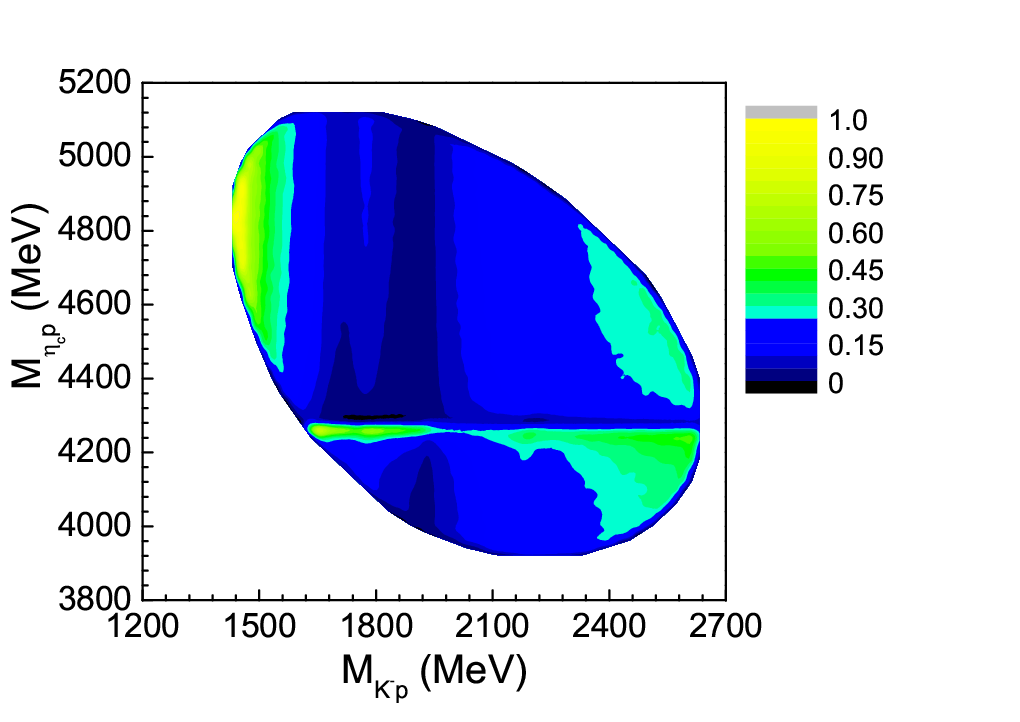
In Fig. 5, we show the Dalitz plot for the invariant masses of $\eta_{c}p$ and $K^{-}p$. In the figure we can see clearly the signals for the $\Lambda(1405)$ in $K^{-}p$, close to the $K^{-}p$ threshold and in $\eta_{c}p$ for the resonance $R$.

In Fig. 6 we show the invariant mass distribution for $K^{-}p$ ($M_{\rm inv}\equiv M_{K^{-}p}$) and $\pi\Sigma$ ($M_{\rm inv}\equiv M_{\pi\Sigma}$). We stress once more that the $K^{-}p$ is only for $s$-wave, related to the $\Lambda(1405)$ production close to threshold. We can expect extra strength from $\Lambda(1520)$ excitation and other resonances, but with the partial wave anlysis of LHCb one can separate the contributions of different resonances as done for the $\Lambda^{0}_{b}\to J/\psi K^{-}p$ reaction [2, 1], and compare with our results. Very interesting is to compare the strength and shape of $\pi\Sigma$ production with $K^{-}p$. The results for the $\pi\Sigma$ mass distribution deserve some attention. The three distributions for $\pi^{+}\Sigma^{-}$, $\pi^{0}\Sigma^{0}$, and $\pi^{-}\Sigma^{+}$ are very similar, they peak at the same energy and appear with no background. This is a consequence of the dynamics of their production. Indeed, in Eq. (1) we see that $\pi\Sigma$ is not produced at tree level. It is only produced by rescattering as seen in Eq. (8). This means that the $\Lambda(1405)$ resonance is produced clearly without background from tree level. Second, since we saw that in the final meson-baryon states we had $I=0$, this means that the $\pi\Sigma$ is produced in $I=0$ without contribution of $I=1$, for instance the $\Sigma(1385)$ or other $I=1$ background sources. This is actually a problem in many reactions producing the $\Lambda(1405)$, as photoproduction [69] or the $pp\to pK^{-}\pi\Sigma$ reaction [70]. One good consequence of this is that the different $\pi^{+}\Sigma^{-}$, $\pi^{0}\Sigma^{0}$, and $\pi^{-}\Sigma^{+}$ are produced with similar strength and peaking at the same place, which does not occur when there is contribution from both $I=0$ and $I=1$ [71]. There is another interesting feature which is that all these distributions peak at $1420$ MeV. This is a consequence of the dynamics of the $\Lambda(1405)$ and the two states (two poles in the same Rieman sheet) that are associated to it [72, 73]. In these chiral pictures, corroborated by all works in chiral dynamics, ³³ 3 See the chapter ”pole structure of the $\Lambda(1405)$ region” of the PDG [68]. there are two states, one with mass around $1420$ MeV, that couples strongly to $\bar{K}N$, and the other one at around $1385$ MeV that couples mostly to $\pi\Sigma$. The dynamics of the present reaction is such that the $\Lambda(1405)$ is initially produced by $\bar{K}N$ (see Eq. (3) and Eq. (8)), hence, it is basically the $\Lambda^{*}$ state at $1420$ MeV the one which is excited, and this is seen in Fig. 6. This selection of the upper $\Lambda^{*}$ states also occur, and is supported experimentally, in other reactions where the $\Lambda(1405)$ is initiated by the $\bar{K}N$ channel, as the $K^{-}p\to\pi^{0}\pi^{0}\Sigma^{0}$ reaction [74, 75] or the $K^{-}d\to n\pi\Sigma$ reactions [76, 77]. The discussion done here indicates that the present reaction, $\Lambda^{0}_{b}\to\eta_{c}\pi\Sigma$, is an ideal one to show in a very clean way the upper state of the two $\Lambda(1405)$ states.

Finally, in Fig. 7, we show the mass distribution of $\eta_{c}p$. We see a strong and clear peak around the mass of the dynamically generated hidden charm resonance $M_{R}=4265$ MeV. The peak has a large strength, bigger than the $K^{-}p$ strength at the peak, which indicates that it should be clearly visible. This is the comparison we want to make, and not the comparison of the strengths of the peak with the background, because the background in Fig. 7 is obviously underestimated since we do not consider the excitation of other $\Lambda^{*}$ apart from the $\Lambda(1405)$, which would fill the region below the peak in Fig. 7 with extra background. We should also warn that the mass of $R$ in Refs. [3, 4] is a prediction, but one has uncertainties in the mass, tied to the choice of the subtraction constant. Uncertainties of about 20 MeV, or even more, are expected, but the stability of the strength of the peak has been studied in similar reactions producing hidden charm states [41, 42, 43] and the same should happen here.

We have not cared about the absolute normalization in the work. However, there is an interesting exercise that we can do. Since $\eta_{c}$ and $J/\psi$ are both $c\bar{c}$ states which differ only in the spin alignments, we can use heavy quark spin symmetry (HQSS) to relate the reactions $\Lambda^{0}_{b}\to J/\psi K^{-}p$ and $\Lambda^{0}_{b}\to\eta_{c}K^{-}p$. Semileptonic decays have been investigated within the HQSS formalism [78, 79]. The nonleptonic decay with the internal emission topology is more complicated, because it has two quark vertices, rather than one in the semileptonic decay. We have done our own formulation of the problem, using Racah algebra and we show the derivation in the Appendix. The conclusion is that the rate of $\Lambda^{0}_{b}\to\eta_{c}K^{-}p$ production with $K^{-}p$ in $S$-wave is three times bigger than for $\Lambda^{0}_{b}\to J/\psi K^{-}p$ apart from phase space. This information is useful because the $\Lambda^{0}_{b}\to J/\psi K^{-}p$ has been investigated in LHCb [2, 1] and thus we should expect strengths for the $\Lambda^{0}_{b}\to\eta_{c}K^{-}p$ reaction reasonably bigger than for $\Lambda^{0}_{b}\to J/\psi K^{-}p$.

We have performed a study of the $\Lambda^{0}_{b}\to\eta_{c}K^{-}p$ and $\Lambda^{0}_{b}\to\eta_{c}\pi\Sigma(\pi^{+}\Sigma^{-},\pi^{0}\Sigma^{0},\pi^{-}\Sigma^{+})$ reactions. We identify the mechanism for the reaction at quark level and see that the $K^{-}p$ produced couples only to $\Lambda^{*}$ states and not $\Sigma^{*}$ states. The Cabibbo favored mechanism (up to the $bcW$ vertex, necessary for the weak decay) produces an $sud$ cluster in the final state that, upon hadronization, leads to $K^{-}p$, $\pi^{+}\Sigma^{-}$, $\pi^{0}\Sigma^{0}$, and $\pi^{-}\Sigma^{+}$ in the final state, and this interaction is basically mediated by the $\Lambda(1405)$ state of high mass at $1420$ MeV, such that the different $\pi\Sigma$ channels show invariant mass distributions peaking at this energy. We emphasize that the reaction is a very clean one to produce this resonance, free of contributions from $I=1$ sources.

We also take into account the $\eta_{c}p$ interaction, which is enhanced close to a dynamically generated resonance $R$, from the $\bar{D}\Sigma_{c}$, $\bar{D}\Lambda_{c}$, and $\eta_{c}N$ channels, due to a relatively large coupling of the resonance to $\eta_{c}p$, weaker than to $\bar{D}\Sigma_{c}$ (the largest component) but larger than the coupling to the $\bar{D}\Lambda_{c}$ channel.

Up to a global normalization constant, we can compare the strength of the reactions in the $K^{-}p$ mass distribution close to the $K^{-}p$ threshold, the strength of the $\pi^{+}\Sigma^{-}$, $\pi^{0}\Sigma^{0}$, and $\pi^{-}\Sigma^{+}$ mass distributions around the peak of the upper $\Lambda(1405)$ state and the strength of the $\eta_{c}p$ mass distribution at the peak of the $R$ resonance around $4265$ MeV. They all have a similar strength and should be easily identifiable.

The results shown here are predictions for ongoing experiments at LHCb, and comparison of the observed results with these predictions will be most useful to pin down the different dynamical aspects of hadron physics that we have discussed in this paper.

We would like to thank L. Zhang for suggesting this problem. This work is partly supported by the National Natural Science Foundation of China (Grants No. 11475227, 11565007, 11647309, 11735003) and the Youth Innovation Promotion Association CAS (No. 2016367). This work is also partly supported by the Spanish Ministerio de Economia y Competitividad and European FEDER funds under the contract number FIS2011-28853-C02-01, FIS2011- 28853-C02-02, FIS2014-57026-REDT, FIS2014-51948-C2- 1-P, and FIS2014-51948-C2-2-P, and the Generalitat Valenciana in the program Prometeo II-2014/068. We acknowledge the support of the European Community-Research Infrastructure Integrating Activity Study of Strongly Interacting Matter (acronym HadronPhysics3, Grant Agreement n. 283286) under the Seventh Framework Programme of EU.

We write the operator responsible for the transition of Fig. 1 and make the HQSS approach neglecting the terms of $1/m_{Q}$ ($m_{Q}$, the heavy quark mass). Considering the $W$ propagator as $D_{W}=g_{\mu\nu}/m^{2}_{W}$, we must evaluate matrix elements of the type

Making the non relativistic reduction of the $\gamma_{\mu}$ and $\gamma_{\mu}\gamma_{5}$ matrices and keeping terms of order ${\mathcal{O}}(1)$ we must keep, $\gamma^{0}\sim 1$ and $\gamma^{i}\gamma_{5}\sim\sigma^{i}$ ($i=1$, 2, 3). Thus we have to evaluate the following matrix element

where $S_{1}$ and $S_{2}$ are the third components of the spins of the $c$, $\bar{c}$, and $M$ and $M^{\prime}$ are the third spin components of the $b$ and $s$ quarks, respectively.

We next write

where $\sigma^{\mu}$ are the Pauli matrices in the spherical basis and using the Wigner Eckert theorem we have

The other consideration is that we have to combine particle-antiparticle in angular momentum. We then take into account that the state $<J,-M|(-1)^{J+M}$ behaves like a state $|JM>$. Then we combine a state with $S_{1}$ and $-S_{2}$ to form $|jm>$, the $\eta_{c}$ or $J/\psi$ state with $j=0$ or $1$, respectively.

Then Eq. (10) becomes

which implies in both terms $M^{\prime}=M-m$, as it should be.

Next one reorders the Clebsch-Gordan coefficients to produce a Racah coefficient [80] as done in Ref. [81] and we find

with $C=-2$ and $2$ for $j=0$ and $1$, respectively.

In addition one has the radial matrix element

with $c_{1}$ and $c_{2}$ corresponding to the $c$, $\bar{c}$ quarks and $b$, $s$ to the $b$, $s$ quarks, while $q$ is the momentum transfer and we have assumed that the $s$ quark is in $l=0$, as if we were producing the $\Lambda$ ground state.

When we produce $\eta_{c}K^{-}p$ with $K^{-}p$ in $S$-wave, the final state $K^{-}p$ must be obtained from the hadronization, as shown in Fig. 2, but since $K^{-}p$ in $S$-wave has negative parity the $s$ quark prior to the hadronization must have negative parity because the $ud$ quark pair is spectator and has positive parity. Then one has to have the $s$ quark excited to $l$ odd and we take $l=1$, the lowest one, which leads to $J=1/2$ that one has with $K^{-}p$ in $S$-wave. Eq. (13) is generalized in this case and we find

where $J$ is the $s$ total spin that comes from the combination of spin and the $l$ angular momentum of the $s$ quark, and $M^{\prime}$ its third component. The radial matrix element now becomes

The next step is to combine $|jm>$ with $|1/2,M-m>$ to give the initial $|\frac{1}{2},M>$ state in the case of $s$ quark with $l=0$, multiplying by the Clebsch-Gordan coefficient ${\mathcal{C}}(j\frac{1}{2}\frac{1}{2};m,M-m)$ and summing over $m$. The resulting amplitude becomes

which indicates that the $J/\psi$ production in this case would be three times bigger than for $\eta_{c}$.

On the other hand, in the case we are concerned about, with the $s$ quark in $l=1$, we must combine $|jm>$ with $|JM^{\prime}>$ to give $|\frac{1}{2}M>$, multiplying by the Clebsch-Gordan coefficient ${\mathcal{C}}(jJ\frac{1}{2};m,M^{\prime},M)$ and summing over $m$. This makes $M^{\prime}=M-m$. Once again we recombine the three Clebsch-Gordan coefficients into one Clebsch-Gordan and one Racah coefficient, $W(1\frac{1}{2}\frac{1}{2}j;\frac{1}{2}\frac{1}{2})$, with the final result for the amplitude for $J=1/2$ ($K^{-}p$ in $S$-wave),

with $C^{\prime}=\sqrt{2}$ for $j=0$ and $C^{\prime}=-\frac{\sqrt{6}}{3}$ for $j=1$. Since $|\mathcal{C}(1\frac{1}{2}\frac{1}{2};0M)|^{2}$ is independent of $M$, the probability to production $\eta_{c}K^{-}p$ in $S$-wave is now three times bigger than for $J/\psi K^{-}p$.

References

- [1] R. Aaij et al. [LHCb Collaboration], Phys. Rev. Lett. 115, 072001 (2015).
- [2] R. Aaij et al. [LHCb Collaboration], Chin. Phys. C 40, 011001 (2016).
- [3] J. J. Wu, R. Molina, E. Oset and B. S. Zou, Phys. Rev. Lett. 105, 232001 (2010).
- [4] J. J. Wu, R. Molina, E. Oset and B. S. Zou, Phys. Rev. C 84, 015202 (2011).
- [5] Z. C. Yang, Z. F. Sun, J. He, X. Liu and S. L. Zhu, Chin. Phys. C 36, 6 (2012).
- [6] C. Garcia-Recio, J. Nieves, O. Romanets, L. L. Salcedo and L. Tolos, Phys. Rev. D 87, 074034 (2013).
- [7] C. W. Xiao, J. Nieves and E. Oset, Phys. Rev. D 88, 056012 (2013).
- [8] T. Uchino, W. H. Liang and E. Oset, Eur. Phys. J. A 52, 43 (2016).
- [9] M. Karliner and J. L. Rosner, Phys. Rev. Lett. 115, 122001 (2015).
- [10] S. G. Yuan, K. W. Wei, J. He, H. S. Xu and B. S. Zou, Eur. Phys. J. A 48, 61 (2012).
- [11] R. Chen, X. Liu, X. Q. Li and S. L. Zhu, Phys. Rev. Lett. 115, 132002 (2015).
- [12] L. Roca, J. Nieves and E. Oset, Phys. Rev. D 92, 094003 (2015).
- [13] J. He, Phys. Lett. B 753, 547 (2016).
- [14] H. Huang, C. Deng, J. Ping and F. Wang, Eur. Phys. J. C 76, 624 (2016).
- [15] U. G. Meißner and J. A. Oller, Phys. Lett. B 751, 59 (2015).
- [16] C. W. Xiao and U.-G. Meißner, Phys. Rev. D 92, 114002 (2015).
- [17] M. I. Eides, V. Y. Petrov and M. V. Polyakov, Phys. Rev. D 93, 054039 (2016).
- [18] G. Yang and J. Ping, Phys. Rev. D 95, 014010 (2017).
- [19] R. Chen, X. Liu and S. L. Zhu, Nucl. Phys. A 954, 406 (2016).
- [20] Q. F. Lü and Y. B. Dong, Phys. Rev. D 93, 074020 (2016).
- [21] Y. Shimizu, D. Suenaga and M. Harada, Phys. Rev. D 93, 114003 (2016).
- [22] C. W. Shen, F. K. Guo, J. J. Xie and B. S. Zou, Nucl. Phys. A 954, 393 (2016).
- [23] C. W. Xiao, Phys. Rev. D 95, 014006 (2017).
- [24] R. Chen, J. He and X. Liu, Chin. Phys. C 41, 103105 (2017).
- [25] J. Wu, Y. R. Liu, K. Chen, X. Liu and S. L. Zhu, Phys. Rev. D 95, 034002 (2017).
- [26] Y. Shimizu and M. Harada, Phys. Rev. D 96, 094012 (2017).
- [27] Y. Yamaguchi, A. Giachino, A. Hosaka, E. Santopinto, S. Takeuchi and M. Takizawa, Phys. Rev. D 96 (2017), 114031.
- [28] R. F. Lebed, Phys. Lett. B 749, 454 (2015).
- [29] R. Zhu and C. F. Qiao, Phys. Lett. B 756, 259 (2016).
- [30] A. Mironov and A. Morozov, JETP Lett. 102, 271 (2015) [Pisma Zh. Eksp. Teor. Fiz. 102, 302 (2015)].
- [31] S. M. Gerasyuta and V. I. Kochkin, arXiv:1512.04040 [hep-ph].
- [32] E. Santopinto and A. Giachino, Phys. Rev. D 96, 014014 (2017).
- [33] P. G. Ortega, D. R. Entem and F. Fernández, Phys. Lett. B 764, 207 (2017).
- [34] H. X. Chen, W. Chen, X. Liu, T. G. Steele and S. L. Zhu, Phys. Rev. Lett. 115, 172001 (2015).
- [35] K. Azizi, Y. Sarac and H. Sundu, Phys. Rev. D 95, 094016 (2017).
- [36] E. J. Garzon and J. J. Xie, Phys. Rev. C 92, 035201 (2015).
- [37] A. N. Hiller Blin, C. Fernández-Ramírez, A. Jackura, V. Mathieu, V. I. Mokeev, A. Pilloni and A. P. Szczepaniak, Phys. Rev. D 94, 034002 (2016).
- [38] A. Ali, I. Ahmed, M. J. Aslam and A. Rehman, Phys. Rev. D 94, 054001 (2016).
- [39] V. Kubarovsky and M. B. Voloshin, arXiv:1609.00050 [hep-ph].
- [40] X. H. Liu and M. Oka, Nucl. Phys. A 954, 352 (2016).
- [41] H. X. Chen, L. S. Geng, W. H. Liang, E. Oset, E. Wang and J. J. Xie, Phys. Rev. C 93, 065203 (2016).
- [42] A. Feijoo, V. K. Magas, A. Ramos and E. Oset, Eur. Phys. J. C 76, 446 (2016).
- [43] J. X. Lu, E. Wang, J. J. Xie, L. S. Geng and E. Oset, Phys. Rev. D 93, 094009 (2016).
- [44] Y. H. Lin, C. W. Shen, F. K. Guo and B. S. Zou, Phys. Rev. D 95, 114017 (2017).
- [45] M. Cleven, V. K. Magas and A. Ramos, Phys. Rev. C 96, 045201 (2017).
- [46] T. J. Burns, Eur. Phys. J. A 51, 152 (2015).
- [47] H. X. Chen, W. Chen, X. Liu and S. L. Zhu, Phys. Rept. 639, 1 (2016).
- [48] A. Esposito, A. Pilloni and A. D. Polosa, Phys. Rept. 668, 1 (2016).
- [49] E. Oset et al., Nucl. Phys. A 954, 371 (2016).
- [50] A. Ali, J. S. Lange and S. Stone, Prog. Part. Nucl. Phys. 97, 123 (2017).
- [51] P. Zhou, Y. K. Hsiao and C. Q. Geng, Annals Phys. 383, 278 (2017).
- [52] J. X. Lu, L. S. Geng and M. P. Valderrama, arXiv:1706.02588 [hep-ph].
- [53] S. L. Olsen, T. Skwarnicki and D. Zieminska, arXiv:1708.04012 [hep-ph].
- [54] F. K. Guo, C. Hanhart, U. G. Meißner, Q. Wang, Q. Zhao and B. S. Zou, arXiv:1705.00141 [hep-ph].
- [55] R. F. Lebed, R. E. Mitchell and E. S. Swanson, Prog. Part. Nucl. Phys. 93, 143 (2017).
- [56] F. K. Guo, U. G. Meißner, W. Wang and Z. Yang, Phys. Rev. D 92, 071502 (2015).
- [57] X. H. Liu, Q. Wang and Q. Zhao, Phys. Lett. B 757, 231 (2016).
- [58] M. Bayar, F. Aceti, F. K. Guo and E. Oset, Phys. Rev. D 94, 074039 (2016).
- [59] L. Roca, M. Mai, E. Oset and U. G. Meißner, Eur. Phys. J. C 75, 218 (2015).
- [60] L. Roca and E. Oset, Eur. Phys. J. C 76, 591 (2016).
- [61] L. Zhang, privite communication.
- [62] F.E. Close, Academic Press/London, 1979, 481p.
- [63] K. Miyahara, T. Hyodo, M. Oka, J. Nieves and E. Oset, Phys. Rev. C 95, 035212 (2017).
- [64] R. P. Pavao, W. H. Liang, J. Nieves and E. Oset, Eur. Phys. J. C 77, 265 (2017).
- [65] L. L. Chau, Phys. Rept. 95, 1 (1983).
- [66] E. Oset and A. Ramos, Nucl. Phys. A 635, 99 (1998).
- [67] G. Ecker, Prog. Part. Nucl. Phys. 35, 1 (1995).
- [68] C. Patrignani et al. [Particle Data Group], Chin. Phys. C 40, 100001 (2016).
- [69] K. Moriya et al. [CLAS Collaboration], Phys. Rev. C 88, 045201 (2013) Addendum: [Phys. Rev. C 88, 049902 (2013)].
- [70] G. Agakishiev et al. [HADES Collaboration], Phys. Rev. C 87, 025201 (2013).
- [71] J. C. Nacher, E. Oset, H. Toki and A. Ramos, Phys. Lett. B 455, 55 (1999).
- [72] J. A. Oller and U. G. Meißner, Phys. Lett. B 500, 263 (2001).
- [73] D. Jido, J. A. Oller, E. Oset, A. Ramos and U. G. Meißner, Nucl. Phys. A 725, 181 (2003).
- [74] S. Prakhov et al. [Crystall Ball Collaboration], Phys. Rev. C 70, 034605 (2004).
- [75] V. K. Magas, E. Oset and A. Ramos, Phys. Rev. Lett. 95, 052301 (2005).
- [76] O. Braun et al., Nucl. Phys. B 129, 1 (1977).
- [77] D. Jido, E. Oset and T. Sekihara, Eur. Phys. J. A 42, 257 (2009).
- [78] E. E. Jenkins, M. E. Luke, A. V. Manohar and M. J. Savage, Nucl. Phys. B 390, 463 (1993).
- [79] G. G. Lu, Y. D. Yang and H. B. Li, Phys. Lett. B 341, 391 (1995).
- [80] E. Rose, Elementary theory for angular momentum, John Wiley and Sons, 1957.
- [81] W. H. Liang, M. Bayar and E. Oset, Eur. Phys. J. C 77, 39 (2017).