Real-Time Feedback-Based Optimization of Distribution Grids: A Unified Approach
Abstract
This paper develops an algorithmic framework for real-time optimization of distribution-level distributed energy resources (DERs). The proposed framework optimizes the operation of both DERs that are individually controllable and groups of DERs (i.e., aggregations) that are jointly controlled at an electrical point of connection. From an electrical standpoint, wye and delta single- and multi-phase connections are accounted for. The algorithm enables (groups of) DERs to pursue given performance objectives, while adjusting their (aggregate) powers to respond to services requested by grid operators and to maintain electrical quantities within engineering limits. The design of the algorithm leverages a time-varying bi-level problem formulation capturing various performance objectives and engineering constraints, and an online implementation of primal-dual projected-gradient methods. The gradient steps are suitably modified to accommodate appropriate measurements from the distribution network and the DERs. By virtue of this approach, the resultant algorithm can cope with inaccuracies in the distribution-system modeling, it avoids pervasive metering to gather the state of non-controllable resources, and it naturally lends itself to a distributed implementation. Analytical stability and convergence claims are established in terms of tracking of the solution of the formulated time-varying optimization problem. The proposed method is tested in a realistic distribution system with real data.
I Introduction
This paper focuses on real-time optimization of heterogeneous distributed energy resources (DERs) in utility-level systems and “soft” microgrids, with the latter referring to community-, campus-, and neighborhood-level systems connected to the rest of the grid through one point of interconnection. This paper seeks contributions in the design of real-time optimization strategies, to offer decision making capabilities that match the time scale of distribution grids with high DER integration. The objective is to allow the maximization of given DER-level and system-level operational objectives, while coping with the variability of ambient conditions and non-controllable energy assets [1].
Centralized and distributed optimization approaches – such as the AC optimal power flow (OPF) – have been developed for distribution grids to compute optimal setpoints for DERs, so that power losses and voltage deviations are minimized and economic benefits to utility and end-users are maximized (see the tutorial [2] and pertinent references therein). Centralized approaches utilize off-the-shelf solvers for nonlinear programs, or leverage convex relaxation and approximation techniques to obtain convex surrogates. Distributed solution methods capitalize on the decomposability of Lagrangian functions to decompose the solution of the optimization task across DERs, utility, and possibly “aggregators.” Either way, these approaches are inadequate for real-time optimization for the following main reasons:
c1) Computational complexity may render impossible the solution of optimization problems on a second (or a few seconds) timescale [2, 3]. In distributed settings, multiple communication rounds are required to reach convergence to a solution.
c2) Conventional optimization tasks operate in an open-loop (i.e., feed-forward) setting, where a grid model and measurements of uncontrollable assets are utilized as inputs. Approximate representation of system physics, modeling errors, and uncertainty in the measurements/forecasts lead to solutions that may be in fact infeasible for the physical power system.
c3) Feed-forward techniques require measurements (or estimation) of the state of non-controllable energy assets everywhere (they are inputs of the optimization problem to be solved). Pervasive metering is impractical in existing distribution grids, and estimation based on limited data might be inaccurate.

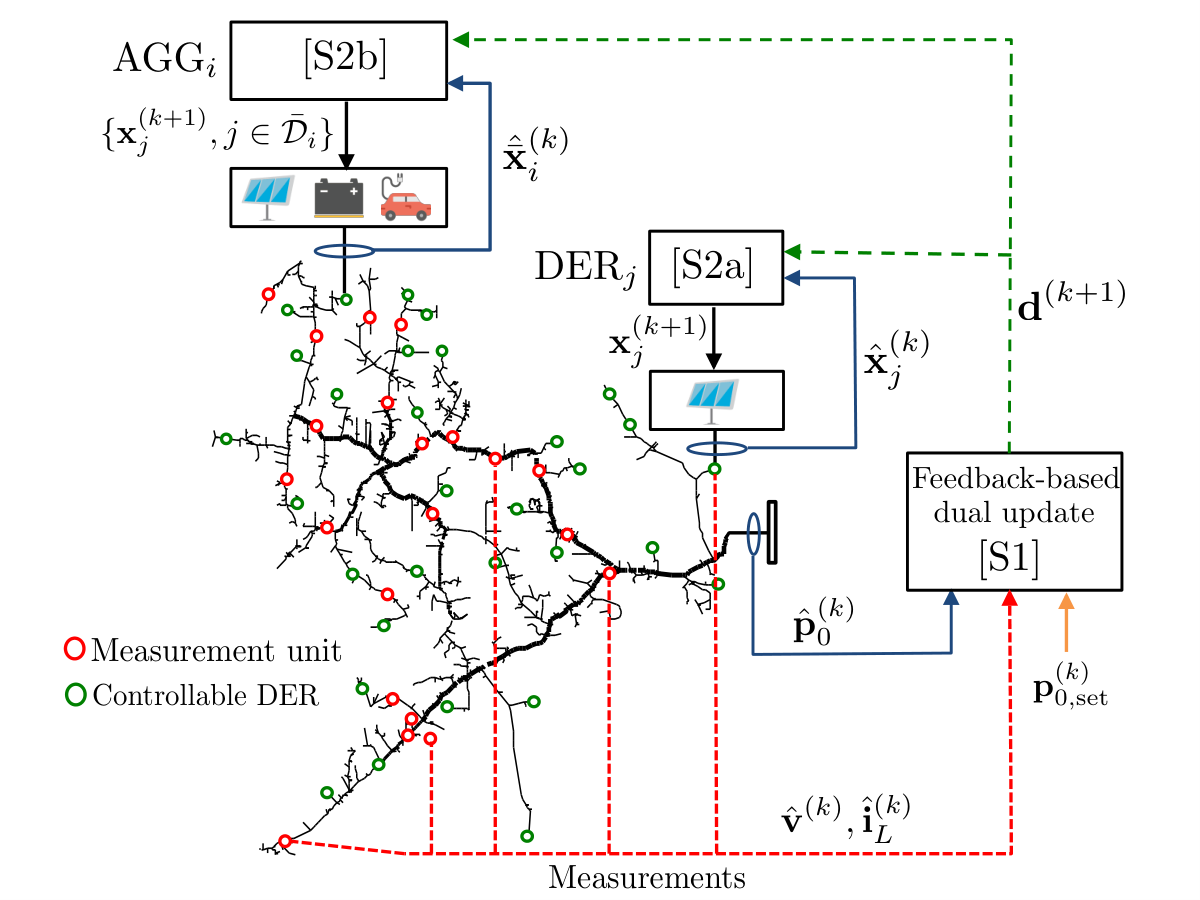
This paper starts from the formulation of a time-varying bi-level convex optimization problem that models optimal operational trajectories of DERs and groups of DERs, and embeds dynamic operational and engineering constraints. The latter include voltage and ampacity limits, feasible operating regions of DERs, and target power flows at the point of interconnection with the rest of the grid (to provide services [4] or partake into market operations). To address the challenge c1), we develop an online algorithm based on a projected primal-dual gradient method to track the optimal solution of the formulated optimization problem. To resolve c2) and c3), the gradient steps are suitably modified to accommodate voltage, power, and current measurements from the distribution network and the DERs – hence the term feedback-based online optimization. The operating principles of the real-time framework are illustrated in Fig. 1. The synthesis of the algorithm leverages the fixed-point linearization method for the multi-phase AC power-flow equations presented in [5], where delta and wye connections are unified under the same mathematical formalism. The resultant algorithm avoids pervasive metering to gather the state of non-controllable resources, it can cope with inaccuracies in the representation of the AC power flows, and it affords a distributed implementation. As illustrated in Fig. 1, analytical convergence and stability claims are established in terms of tracking of the solution of the formulated time-varying optimization problem.
The bi-level nature of the problem allows one to readily optimize the net power generated/consumed by groups of DERs located behind the same meter, while accounting for individual DER constraints. Towards this end, the paper contributes results with respect to the computation of inner approximations of the Minkowski sum of prototypical sets of DERs, to represent the overall feasibility region of groups of DERs; and, a systematic way to compute the gradient of the cost function associated with groups of DERs, along with a mechanism to disaggregate the power command across DERs. With respect to the types of DERs, the paper considers DERs with both continuous and discrete implementable power commands. For the latter, the operational sets of DERs are convexified for the purpose of setpoint computation, whereas implementable setpoints are computed via error-diffusion techniques [6, 7].
General bi-level optimization problems are closely related to the Stackelberg game formulation [8], and are NP-hard even when both the inner and outer optimization problems are convex [9]. There is an extensive literature on such problems in different application domains [10, 11]. In our application, the solution to the inner level optimization problem can be expressed as the solution to the corresponding KKT first order optimality conditions, and hence the problem can be efficiently solved.
The idea of leveraging time-varying problem formulations to model optimal operational trajectories for DERs and developing feedback-based online solvers to track the optimal trajectory traces back to our preliminary works [12, 13] and [14], where time-varying linearized AC OPF formulations were considered for distribution grids. Feedback was in the form of measurements of voltages and powers; while the effectiveness of these methods were shown numerically in [12, 13], analytical tracking results were first provided in [14]. A centralized online algorithm based on a quasi-Newton method was proposed in [15] for a time-varying relaxed non-convex AC OPF (smooth penalty functions were utilized to relax the constraints); considerations regarding estimations of the Hessian were offered. An online incentive-based algorithm was developed in [16] to track a time-varying equilibrium point of a Stackelberg game. Voltage measurements were included into the steps of the alternating direction method of multipliers in [17], and tracking results were established.
For static optimization problems, a feedback-based algorithm for a real-time solution of economic dispatch problems was proposed in [18]; feedback was in the form of measurements of the output powers. Measurements of voltages were considered in the distributed strategy developed in [19], to enforce voltage regulation in distribution networks. Similarly, [20] proposed a distributed reactive power control strategy, and convergence to a solution of a well-posed static optimization problem was analytically established. Local control methods for voltage regulation were proposed in [21]; performance in a dynamic setting was experimentally evaluated. Power measurements were utilized in [22] to dynamically solve a relaxed AC OPF. State measurements were leveraged in [23] to solve an AC OPF for radial systems. Manifold-based approaches were proposed and analyzed in [24, 25] to solve the AC OPF (smooth penalty functions were utilized to relax the constraints); however, the update of the tangent plane in these papers may still require pervasive metering of the non-controllable assets.
The framework in this paper significantly expands our prior works in [14, 26] by providing the following contributions:
i) We consider a bi-level optimization formulation, which is NP-hard problem in general. In particular, the rigorous analysis of online bi-level formulation with feedback is absent in the literature.
ii) We account for aggregations of DERs (e.g., buildings and facilities with multiple DERs behind the meter). We provide new results for the inner approximation of the Minkowski sum of prototypical operational sets for DERs, to represent the overall feasibility set of groups of DERs; we also offer new insights on the computation of the gradient of the aggregate cost function associated with groups of DERs. These results are of independent interest for real-time control applications.
iii) The proposed algorithm is applicable to multi-phase systems with both wye and delta connections.
iv) The proposed framework accommodates DERs with a non-convex (and, in particular, discrete) set of implementable control commands.
v) The proposed framework is tested through numerical simulations based on a real system and using real data from a distribution network located in California in the territory of Southern California Edison.
II Preliminaries and System Model
Notation: Upper-case (lower-case) boldface letters will be used for matrices (column vectors); for transposition; complex-conjugate; and, complex-conjugate transposition. and denote the real and imaginary parts of a complex number, respectively, and . denotes the absolute value of a number or the cardinality of a (discrete) set. For a given vector , takes the absolute value entry-wise; ; and, returns a matrix with the elements of in its diagonal. Given a matrix , denotes its -th entry and denotes the -induced matrix norm. For a function , returns the gradient vector of with respect to . The symbols and denote the vector with all ones and with all zeros, respectively. Given two sets and , denotes the Minkowski sum of and . Finally, given a set , denotes its convex hull; and denotes a closest point to in , namely (the ties can be broken arbitrarily).
II-A DER Model
We consider two classes of DERs: i) devices that are individually controllable; and, ii) groups of DERs that can be controlled as a whole. The second class models, e.g., residential homes and buildings with multiple DERs behind the meter, renewable-based systems with multiple (micro)inverters, and parking garages for EVs. Each DER can be either wye-connected or delta-connected to the network [27], and it can be either single-phase or three-phase. In the following, pertinent notation and modeling details are outlined.
For future developments, let be the set of possible connections, with pertaining to wye connections (line to ground) and referring to delta connections (line to line).
Individually-controllable DERs. Let be the set of individually-controllable DERs, and let collect the real and reactive power setpoint of DER . The DER can be either wye-connected or delta-connected to the network. Three-phase DERs are assumed to operate in a balanced setting; thus, the setpoint is the same across phases. The set collects the phases where DER is connected.
We denote as the set of possible power setpoints for the DER ; the set captures hardware and operational constraints and it is assumed to be convex and compact. It is assumed that the DERs are endowed with controllers that are designed so that, upon receiving the setpoint , the output powers are driven to the commanded setpoints; relevant dynamical models for the output powers of an inverter-interfaced DER are discussed in e.g., [28, 29] and can be found in datasheets of commercially available DERs.
For an inverter-interfaced DER, we consider the following prototypical representation of the set :
| (1) |
where , , and are given DER-dependent parameters. For example, for a PV system represents the inverter capacity, , and is the available real power. For an energy storage systems, represents the inverter rating, and are updated during the operation of the battery based on its internal state (such as the state of charge or DC voltage). Notice that the set is typically time varying, as the parameters , , and vary over time based on ambient conditions and/or internal DER state.
On the other hand, we consider the following operating region for DERs with controllable active powers (e.g., variable speed drives and EVs; see other examples in [30]):
| (2) |
DERs with nonconvex (discrete) controls. Consider a DER with a nonconvex operating region, . This is the case, for example, for (residential) HVAC systems where , or EVs with discrete charging levels. For these devices, the set is the convex hull of ; i.e., . For example, for an HVAC systems we have that [cf. (2)]. The algorithm proposed in Section III will utilize a randomization procedure to recover implementable setpoints based on [31, 32]. For a DER with nonconvex set of implementable setpoints, denotes an implementable setpoint, whereas is a (relaxed) setpoint computed based on the convex hull of . Notice that for devices that lock on a state due to engineering or operational constraints, the set is a singleton over a given period of time; for example, if an HVAC system is required not to switch ON for a few minutes, then for a given interval .
Aggregations of DERs. Suppose that the distribution grid features a set of residential homes, building, or other facilities with multiple DERs that are controlled jointly. Let denote the set of devices within the th aggregation, and define as the setpoint for the net powers generated by the DERs within a group. The set collects the connections of the aggregation .
Let be either the exact Minkowski sum of the operating regions of the DERs within the th aggregation or an inner approximation thereof. In the following, we provide pertinent results for the Minkowski sum of sets (1) and (2). There is extensive literature on devising generic numerical methods to compute aggregated flexibility regions using Minkowski sums [33, 34, 35]. The goal in this paper is rather to develop a simple analytical approximation that can be directly used in real-time algorithms.
First, notice that the Minkowski sum of two sets and for two DERs with controllable active powers is given by:
| (3) |
The following theorems deal with the Minkowski sums and .
Proposition 1.
Proposition 2.
Inner and outer approximations of the Minkowski sum of two sets and are given by
| (5a) | ||||
| (5b) | ||||
for any satisfying the following condition
| (6) |
where , and .
We note that the best choice for in Proposition 2 is given by the upper bound:
The proofs of Propositions 1 and 2 are provided in Appendix -A and -B, respectively. Notice that the inner approximation is convex and compact, and it is in the form of (1).
Expression (3) along with the results of Propositions 1 and Theorem 2 can be utilized to compute an inner approximation of the feasible region of the net powers for each aggregation of DERs . For example, the feasible region for the net powers generated by a residential house with a PV system, a battery, and an EV can be computed by first leveraging (5a) to sum the sets pertaining to the PV system and the battery and subsequently (4), to add up the feasible region of the EV.
II-B Network Model
We consider a generic multi-phase distribution network with multiphase nodes collected in the set , , and distribution lines represented by the set of edges . Node denotes the three-phase slack bus, i.e., the point of connection of the distribution grid with the rest of the electrical system. At each multiphase node, controllable and non-controllable devices can be either wye- or delta-connected [27].
We briefly showcase the set of AC power-flow equations for this generic setting (a comprehensive description can be found in, e.g., [27] and [5]). To this end, let be a vector collecting the line-to-ground voltages in all phases of the nodes in ; similarly, vector collects all the phase net current injections, the phase-to-phase currents in all the delta connections, and vectors and collect the net complex powers injected at nodes from devices with wye and delta connections, respectively. With these definitions in place, the AC power-flow equations can be compactly written as:
| (7a) | |||
| (7b) | |||
where , and are the submatrices of the admittance matrix
| (8) |
which can be formed from the topology of the network and the -model of the distribution lines [27]; is the total number of single-phase connections, and is a block-diagonal matrix mapping the direction of the currents in the delta connections; see [5, 36] for a detailed description.
The nonlinearities in (7) hinder the possibility of seeking analytical closed-form solutions to pertinent electrical quantities such as voltages, power flows, and line currents as a function of the DERs’ power injections. To facilitate the design and analysis of real-time optimization methods, we leverage the approximate linear models proposed in [5, 37]. To this end, denote as the vector collecting the phase-to-ground voltages at given measurement points ; the vector collecting the line currents for a subset of monitored distribution lines (or given by pseudo-measurements); and, the vector of real powers entering node on the phases . Then, (where the absolute value is taken entry-wise), , and can be approximately expressed as:
| (9a) | ||||
| (9b) | ||||
| (10a) | ||||
| (10b) | ||||
| (11a) | ||||
| (11b) | ||||
where collects the net non-controllable active and reactive powers at connection of node , and stack all the setpoints and , respectively, and the matrices , , , , , along with the vectors , , and are model parameters that can be computed through e.g., the fixed-point linearization method proposed in [5, 37]; for brevity, we defined the matrices , , , , , and . As explained in [5, 37], these model parameters capture the effects of different types of connection (e.g., wye or delta) and can be computed based on the admittance matrix of the system. If a fixed-point linearization method is utilized, knowledge of the non-controllable powers is not required for the computation of the model parameters. If only wye connections are present, an alternative way to obtain (9)–(11) is presented in, e.g., [38].
It is worth emphasizing that the approximate models (9)–(11) are utilized to facilitate the design and the performance analysis of the real-time algorithm. In Section III, we show how to leverage measurements from the distribution grid and DERs to cope with the inaccuracies introduced by a linear approximation of the AC power flows; whereas in Section IV, we establish appropriate stability claims.
III Feedback-based Dynamic Optimization
We design a new real-time optimal power flow method where power setpoints of the DERs are updated on a second timescale [39, 14, 15] to maximize operational objectives while coping with the variability of ambient conditions and non-controllable assets. Consider then discretizing the temporal domain as , where and will be taken to be the time required to compute one closed-loop iteration of the proposed algorithm. As discussed shortly, the value of is based on underlying communication delays, as well as operational considerations of utility and aggregators.
We next leverage the time-varying optimization formalism [40, 14] to model optimal operational trajectories for the DERs, based on 1) possibly time-varying optimization objectives and operational constraints, as well as 2) variability of non-controllable assets and ambient conditions. Hereafter, the superscript (k) will be utilized to indicate variables, functions, and inputs at time , for all .
III-A Formalizing Optimal Operational Trajectories
Let and be given limits for the magnitude of phase-to-ground voltages (e.g., ANSI C.84.1 limits), and let be a vector collecting the ampacity limits for the monitored distribution lines. Finally, indicates whether the distribution grid is requested to follow a setpoint for the real powers at the three phases of the point of connection with the rest of the electrical network [4, 41]. When , the sequence of setpoints shall be tracked within a given accuracy . With these definition, the following time-varying optimization problem is formulated to model optimal operational trajectories for the DERs:
| (12a) | ||||
| (12b) | ||||
| (12c) | ||||
| (12d) | ||||
| (12e) | ||||
| (12f) | ||||
| (12g) | ||||
| (12h) | ||||
where we recall that is a convex set modeling hardware constraints of the DER at a given time ; is a time-varying convex function associated with the DER ; and, the function associated with the th aggregation of DERs is defined as follows:
| (13a) | ||||
| (13b) | ||||
| (13c) | ||||
Problem (13) is utilized to disaggregate the setpoint across the DERs .
i) when set is given by the (exact) Minkowski sum of , (12)–(13) is equivalent to a “flat” optimization strategy where (12) does not consider points of aggregation (the flat formulation includes individual optimization variables and constraints for each one of the DERs; see e.g., [23, 12, 14, 30]);
ii) if the set is an inner approximation of the Minkowski sum, then (12)–(13) represents a restriction of the “flat” optimization problem.
Problem is a time-varying convex optimization problem; however, solving in a batch fashion at each time might be impractical because of the following three main challenges:
c1: Complexity. For real-time implementations (e.g., when is on the order of a second or a few seconds), it might be impossible to solve to convergence; this is especially the case of distributed settings, where multiple communication rounds are required to reach convergence.
c2. Model inaccuracy. Feed-forward (i.e., open-loop) solution of suffers from inaccuracies due approximate linear models (9)–(11), as well as estimation errors for the admittance matrix and loads.
c3. Pervasive metering. Solving (either in a batch form or online) requires collecting measurements of the (aggregate) noncontrollable loads at all locations in real time, in order to compute (9)-(11) [2].
In the following, we present a feedback-based online algorithm that tracks the optimal solution of over time, while coping with model inaccuracies and avoiding ubiquitous metering.
III-B Real-time Algorithm
The following assumption is imposed throughout the paper.
Assumption 1.
For each DER , and for each DER in the aggregation :
A1.i the set is convex and compact for all ;
A1.ii the function is convex and continuously differentiable, and its gradient is Lipschitz continuous for all .
Assumption 2.
See Appendix -C for an example of problems that satisfy the assumption above; see also [42] for analytical conditions and more elaborate examples.
We next outline results pertaining to the DER aggregations .
Lemma 1.
Theorem 1.
Theorem 2.
Proofs are provided in the Appendix. The results of Theorem 1 and Theorem 2 are valid at each time instant . These results will be utilized in the design of the real-time algorithm to update the aggregate setpoints of groups of DERs. They will also be leveraged to establish pertinent convergence and stability claims in Section IV.
Let , and be the dual variables associated with constraints (12d), (12e), (12f), (12g), and (12h), respectively. The Lagrangian function associated with the problem (12) at time is given by:
where for simplicity of exposition and is a vector of ones of appropriate dimensions. Consider the following regularized Lagrangian function, where are regularization factors:
| (15) |
and notice that is strongly convex in the primal variables and strongly concave in the dual variables. Consider then the following time-varying saddle-point problem:
| (16) |
and let denote the unique primal-dual optimizer of (16). Similar to e.g., [14, 26], the design of the online algorithm leverages appropriate modifications of online projected-gradient methods to track the time-varying solution of (16). Although the optimizer of (16) is expected to be different from optimizers of the original problem, in Section IV we will show that the strong convexity and concavity of will enable the real-time algorithm to achieve Q-linear convergence. The discrepancy between and the solution of problem can be bounded as shown in [43]. The point is closely related to the so-called approximate Karush-Kuhn-Tucker (KKT) conditions (see, for example, [44]).
Let be a given step size. Then, given the results of Theorem 1 and based on the regularized time-varying saddle-point formulation (16), the execution of the following steps at each time defines the proposed online algorithm. The algorithm produces power setpoints for the DERs at each time , .
Real-time optimization algorithm
At each perform the following steps:
[S1a]: Collect voltage measurements at given measurement points and perform the following updates:
| (17) | ||||
| (18) |
[S1b]: Obtain measurements or estimates of on lines of interest and perform the following updates:
| (19) |
[S1c]: Collect measurements at the point of common coupling and perform the following updates:
| (20) | ||||
| (21) |
[S2a]: Each device performs the following steps:
-
[S2a.1] Measure output powers
-
[S2a.2] Update power setpoints as follows:
(22) -
[S2a.3] If DER has a set of discrete setpoints, compute the implementable setpoint as:
(23) (24) -
[S2a.4] Command setpoint to the DER.
[S2b]: Each DER aggregation performs the the following steps:
-
[S2b.1] Measure aggregate output powers
-
[S2b.2] Update setpoints for the aggregate powers :
(25) -
[S2b.3] Given the aggregate powers , compute the setpoints of the individual DERs and the new vector by solving the saddle-point problem:
(26) -
[S2b.4] If DER has a set of discrete setpoints, compute the implementable setpoint as:
(27) (28) -
[S2b.5] Command setpoints to the DERs.
[S3]: Go to [S1].
The following remarks are in order:
- 1.
Notice that the feedback is utilized in the algorithm in steps [S1] and [S2] in the form of measurements of voltages, currents, and power flows at the point of common coupling; these measurements replace the corresponding analytical expressions. By virtue of this approach, challenges (c2)-(c3) are resolved and, in particular, measurement of the state of uncontrollable devices is not required. We note that in its straightforward implementation, the algorithm requires measurements at nodes where there a corresponding constraint is imposed; however, if real-time state estimation procedure is available, the measurements can be replaced with the estimated state.
- 2.
The real-time algorithm affords a distributed implementation as shown in Fig. 2. Once measurements , , and are acquired, step [S1] is performed at the utility/aggregator, which subsequently broadcasts the dual variables . Steps [S2a] and [S2b] are implemented locally at individual DERs and aggregations of DERs (in the Fig. 2, AGG stands for aggregation), respectively.
- 3.
Note that the sub-steps [S1a], [S1b], and [S1c] can be carried out in parallel at the utility/aggregator.
- 4.
The framework is flexible enough so that the entire computation can be performed centrally. However, there are obviously disadvantages to this. First, this creates a single point failure: if the central entity fails, the entire scheme stops working; however, in the distributed implementation, the local controllers can still compute (sub-)optimal setpoints using perhaps outdated network-wide information (i.e., outdated Lagrange multipliers). Second, the centralized implementation requires point-to-point communication with every DER to communicate individual setpoints; on the other hand, distributed implementation advocated here only requires broadcast communication – every DER receives the same Lagrange multiplier. This is especially important when the number of measurement points (or, the points where we want to impose constraints) is much smaller than the number of DERs in the system. Finally, the privacy argument applies here: if we implement the algorithm centrally, the DERs have to reveal their private information (e.g., preferences and feasible regions).
- 5.
The steps (24) and (28) represent the implementation based on the error-diffusion algorithm. In particular, the accumulate error between the continuous setpoint and the discrete implementation is computed and used in the modified projection steps (24) and (28) to obtain the next implementable (discrete) setpoint; see [32] for further details. Finally, notice that steps (24) and (28) involve the solution of a localized nonconvex program to compute implementable commands.
The ability of the algorithm to track the optimizers of (16) is analytically established next.
IV Performance Analysis
We next analyze the proposed algorithm under the assumption of synchronous updates in steps [S1] and [S2] above. The analysis of the asynchronous case can be carried out similarly on expense of heavier notation and further assumptions; see for example [45].
We start by stating the following assumption regarding problem (12).
Assumption 3.
Problem (12) is feasible and Slater’s condition holds at each time , .
Assumption 3 implies that there exists a power flow solution that adheres to voltage and ampacity limits. When the distribution network is required to follow a setpoint at the point of common coupling, Assumption 3 presumes that the setpoint is feasible. Feasibility of the power flow solutions (with and without setpoints for the active and reactive power at the substation) can be assessed by solving suitable optimization problems at a slower time scale; see, for example, the optimization approaches proposed in [46, 41].
Regarding the temporal variability of problem (12), we introduce the following quantity to capture the variation of the optimal solution trajectory over time:
| (29) |
For sufficiently small sampling intervals , can be interpreted as a bound on the norm of the gradient of the optimal solution trajectory with respect to time. In the context of (12), depends on the variability of the cost function, non-controllable loads, as well as available powers from the renewable-based DERs.
Next, since models (9)–(11) are linear and the sets and are compact (cf. Assumption 1), there exist constants , , and such that, for every ,
For future developments, define . Further, notice that from Assumption 1 and Theorem 2, the gradient map is Lipschitz continuous with a given constant over the set . Let , so that
| (30) |
for all , , and , .
Define the errors introduced by the measurement noise and modeling mismatches (i.e., discrepancy between the nonlinear AC power-flow equations and the linearized model, as well as possible inaccurate knowledge of the admittance matrix) as follows:
where we recall that , , and are measurements (or pseudo-measurements). The following assumption is made.
Assumption 4.
There exist finite constants , , , and such that , , , and for all ; that is, the errors are uniformly bounded in time.
As discussed in Section II-A, DERs are presumed to be equipped with embedded controllers that drive the output powers to the commanded setpoints. If the time constant of the controllers is longer than , Assumption (4) bounds the discrepancy between the sampled output power and the commanded setpoint. For future developments, define the vector , and notice from Assumption 4 that , .
Let collect the primal and dual variables produced by the real-time algorithm at time . Based on Assumptions 1–4, the main convergence results are established next.
Theorem 3.
Corollary 1.
If , then the sequence converges Q-linearly to up to an asymptotic error bound given by:
| (33) |
where .
Notice first that the condition is satisfied if:
| (34) |
Also, observe that the value of (and hence knowledge of , and ) is not required in order to satisfy the condition of Corollary 1.
The bound (31) provides a characterization of the discrepancy between and at each time . On the other hand, the asymptotic bound (33) depends on the underlying dynamics of the distribution system through and on the measurement errors through . The result (33) can also be interpreted as input-to-state stability, where the optimal trajectory of the time-varying problem (12) is taken as a reference. When and , the algorithm converges to the solution of the static optimization problem (16). The proof of Theorem 3 is sketched in Appendix -G.
We conclude the section by stating for completeness a result from [32] establishing average tracking properties for the updates (24) and (28).
Theorem 4 (Theorem 2 in [32]).
For each DER with nonconvex operational region there exists a finite constant such that for all . Consequently,
| (35) |
and for all .
Representative numerical experiments using real data are presented in the next section.
V Experiments on a Real System
The proposed real-time algorithm is tested using data of a real distribution feeder located within the territory of Southern California Edison (SCE) As shown in the anonymized diagram in Fig. 3, this distribution feeder features 126 multiphase nodes (excluding the substation), with a total of 366 single-phase points of connection. Wye and delta connections are present at different nodes of the feeder. The feeder has a nominal line-line voltage of 12kV, and it has three phases in all the nodes except the following ones: nodes 63, 67, 68, and 70 have only phases b and c, and nodes 71, 72, 73, and 74 have only phase c (see node numbering in Appendix -H). The feeder serves 362 customers, with a mix of residential, commercial, and industrial facilities. In the numerical experiments, controllable assets include photovoltaic (PV) systems, energy storage systems, and electric vehicles (EVs). Load and irradiance data have a granularity of 6 seconds; to achieve a granularity of 1 second, the time series were interpolated. It follows that the target optimization problem (12)–(13) changes every second.


It is worth pointing out that this feeder is “stiff” and includes only the modelling of the primary side of distribution transformers. Therefore, voltage violations in this feeder are less visible. The main reason for choosing this test case is that this is a real feeder from SCE with real data. The downside is that SCE does not provide any models on the secondary side, where the possibility of the violation is more likely.
The algorithm was coded in Matlab. For a given set of net power injections/consumptions at each of the nodes of the feeder, a power flow solution was obtained using OpenDSS.
The location of the PV and battery systems in the feeder, along with their capacities and connections types, can be found in Appendix -H. In case of multiple PV systems at a node, the devices are aggregated and jointly controlled. Three-phase systems are presupposed to operate in a balanced mode. The operating region of the inverters that accompany PV systems and energy storage systems is in the form of (1). On the other hand, level-2 charging stations for EVs are presupposed, with discrete charging levels of 10, 20, 40, 60, 80, and 100% of the maximum charging capability of 7.2 kW. EVs are located as follows: 5 EVs at node 9, 2 at node 29, and 3 at node 90. The batteries of the EVs have sized of 60, 80, and 130 kWh, and a minimum charging rate is set for the EVs so that they can be fully charged at the time specified by the drivers.
Table I in Appendix -H lists the locations of the PV systems, along with their capacities and connections types; for the latter, the symbol refers to a wye connection on phases and refers to delta connections between the available phases. In case of multiple PV systems at a node, the devices are aggregated and jointly controlled. Three-phase systems are presupposed to operate in a balanced mode. Table II lists the locations of the battery systems, along with the capacity of the inverters, the maximum state of charge, and the connection type. Similarly to PV systems, three-phase batteries operate in a balanced mode. The operating region of the inverters that accompany PV systems and energy storage systems is in the form of (1). On the other hand, level-2 charging stations for EVs are presupposed, with discrete charging levels of 10, 20, 40, 60, 80, and 100% of the maximum charging capability of 7.2 kW. EVs are located as follows: 5 EVs at node 9, 2 at node 29, and 3 at node 90. The batteries of the EVs have sized of 60, 80, and 130 kWh, and a minimum charging rate is set for the EVs so that they can be fully charged at the time specified by the drivers.
The trajectories of individual non-controllable loads and the power available from a PV system with an inverter capacity of 1MW for a selected day in September 2016 are illustrated in Fig. 4. The power available from other PV systems is a scaled version of the trajectory shown in Fig. 4. It can be seen that the selected day is mostly sunny with clear sky; however, clouds introduced a significant variability in the available power from 9:00 to 9:30 and in the afternoon from 15:15 to 16:00. Fig. 5 illustrates the trajectories of the active power at the substation when PV systems are operated at the maximum available power and batteries are not utilized. It can be seen that the feeder is unbalanced, in the sense that there is a discrepancy between the power of phase and that of the remaining phases at the substation. We note that the majority of the controllable assets are three-phase (balanced) with delta connections; hence, it is not possible to balance the operation of the feeder (that is, ensure that the net powers at the three phases of the substation are equal at each point in time).
In the first test, the algorithm is evaluated during the sunny period of the day; in a second test, we test the algorithm during cloudy periods to assess whether it can cope with uncertain (and fast-changing) weather conditions. The PV-related cost functions are set to for three-phase PV systems (with denoting the maximum real power available) and for smaller-size single-phase PV systems. For batteries, and are set to , and for the EVs we have that where is the maximum charging rate. With this setting, the DER will be incentivized to provide services to the grid, while minimizing the power curtailed from the PV systems and the deviation from a predetermined (dis)charging profiles for the batteries. The stepsize is set as and the regularization parameters are and . One step of the algorithm is run every second. PV and battery inverters are presumed to follow a first-order response with a time constant of seconds (hence, a settling time of approximately seconds). Communication delays are set to seconds per link. Voltage limits are set to pu and pu.
In the test cases, we control the DERs in order to track a given trajectory of setpoints at the substation, while ensuring that voltages are within limits. Fig. 6 illustrates the tracking performance of the real-time algorithm from 11:00 to 12:00, where the majority of the problem variability is introduced by non-controllable devices. The red trajectory corresponds to setpoints (which are different across phases to acknowledge the unbalance operation of the feeder), while the powers on the three phases of the substation are color-coded in blue (phase a), green (phase b) and orange (phase c). It can be seen that with the proposed algorithm the power at the substation closely track ramping signals [4] as well as step changes in the setpoints. Similar tracking results are shown in Fig. 7, where we considered the time interval from 15:30 to 16:00, where the the overall power available from the PV systems is varying very fast. In the uncontrolled case in Fig. 5, the variation in the power available from the PV systems translated into spikes in the power at the substation of magnitude up to MW (summed across phases). On the other hand, the algorithm is capable of leveraging energy storage system to lower the power swing. In addition, Fig. 7 reports the tracking result in the case where we increase the capacity of the batteries of 3x. In this case, the algorithm is capable of completely copying with the PV variability (only the phase c is reported to facilitate the comparison between the two cases).
In the previous experiments, voltage magnitudes were well within limits because the feeder is stiff. To test the ability of our method to regulate voltages, we increase the capacity of the PV systems of 3x to create reverse power flow conditions, and we lower the upper limit from to pu. Fig. 8 illustrates the “cloud” of voltages magnitudes across the system for a representative time slot; the blue trajectories represent the voltages magnitudes when the upper limit is pu. It can be seen that the algorithm is capable of regulating voltages while driving the power at the substation to specific setpoints.
VI Concluding Remarks
This paper developed a distributed algorithm for real-time optimization of DERs. The proposed framework optimizes the operation of both DERs that are individually controllable and groups of DERs at an electrical point of connection that are jointly controlled, and it enables (groups of) DERs to pursue given performance objectives while adjusting their (aggregate) powers to respond to services requested by grid operators and to maintain electrical quantities within engineering limits. The design of the algorithm leveraged a time-varying bi-level problem formulation capturing various performance objectives and engineering constraints, and a feedback-based online implementation of primal-dual projected-gradient methods. The resultant feedback-based online algorithm can cope with inaccuracies in the distribution-system modeling, it avoids pervasive metering to gather the state of non-controllable resources, and it naturally lends itself to a distributed implementation. Analytical stability and convergence claims were established in terms of tracking of the solution of the formulated time-varying optimization problem. Future efforts will look at extending the technical findings to time-varying nonconvex problems.
-A Proof of Proposition 1
The proof follows from the fact that the Minkowski sum between a circle and an interval is given by:
where is a concave function given by
-B Proof of Proposition 2
We first prove the outer approximation (5b). Let ; that is, for two DERs and . It can be readily shown that ; further, we have that:
where the first inequality follows by the fact that , , and from the Cauchy-Schwarz inequality; the second inequality holds again by construction. It follows that whenever and ; the converse is, however, not necessarily true.
We next prove the inner approximation (5a). Let . Clearly,
| (36) |
Using the definitions of and , one can verify that
| (37) | |||
| (38) |
Using (38), it follows that
| (39) |
Next, notice that the following inequality holds
| (40) |
and, thus, there exist and such that and so that the inequality (40) holds; consequently, , .. Combining (39) and (40), we require that which, based on (37), can be satisfied by requiring (6) Thus, if satisfies (6), there exists , , such that , which completes the proof.
-C Illustration of Assumption 2
We next provide a simple two-dimensional example in which Assumption 2 is satisfied; for more elaborate examples and further conditions under which this assumption is satisfied, see [42].
Consider an example of problem (13) given by:
| (41a) | ||||
| (41b) | ||||
| (41c) | ||||
for any . We next show that the dual function associated with (41) satisfies Assumption 2. The dual function is given by:
where
It is easy to verify that the explicit solution of this optimization problem is given by:
and the dual function is thus given by:
Note that, for any (i.e., in the interior of the Minkowski sum ), the unique optimal dual variable is given by and it lies in a locally strongly concave region of both and . Also, note that: (i) the dual function is not strongly concave globally, hence the standard results from, e.g. [47, Proposition 12.60], cannot be applied directly; and (ii) if or (i.e., a point on the boundary of the Minkowski sum), in fact there is infinite number of optimal solutions to .
-D Proof of Lemma 1
Notice first that constraint (13c) can be rewritten in a compact form as , where stacks the vectors and the matrix is full row rank.
Let for brevity. From the first-order optimality conditions it follows that
| (42) |
where and are the optimal primal and dual variables, respectively. Notice that is a tall matrix with full column rank; therefore, its left Moore-Penrose pseudoinverse exists. Condition (42) can thus be rewritten as . Taking the norm on both sides and using the Cauchy-Schwarz inequality, one has that
| (43) |
Clearly, by construction. Also, note that: (i) is continuously differentiable by Assumption 1, and (ii) the gradient map is defined over a compact set. Therefore, is a continuous function defined over a compact set, and hence is bounded. This implies that as required. Uniqueness of the optimal dual variable is implied by Assumption 2.
-E Proof of Theorem 1
Convexity of the optimal value function follows [48, Lemma 4.24]. On the other hand, [48, Theorem 4.26] shows that the sub-differential of coincides with the set of optimal dual variables associated with constraint (13c); given [48, Theorem 4.26] and Assumption 2, (14) then follows.
To show that is Lipschitz continuous, notice first that from the convexity of the optimal value function one has that for any . It then follows that
| (44a) | ||||
| (44b) | ||||
Since from Lemma 1, the result readily follows.
-F Proof of Theorem 2
Consider writing the dual function as
| (45) |
where the function is defined as
| (46) |
and the superscript (k) is dropped for brevity. From Assumption 2 (see also [42]), it follows that is locally strongly concave and differentiable; denote as the (local) strong concavity coefficient.
For any feasible and in the interior of the Minkowski sum of , let and denote the corresponding optimal dual variables. From the optimality of and , we have that
| (47) | |||
| (48) |
By using in (47) and in (48), and summing up these two inequalities, we obtain
| (49a) | ||||
| (49b) | ||||
where the last inequality follows by the local strong concavity of around the optimal dual variables. This implies
| (50a) | ||||
| (50b) | ||||
where the second inequality follows from the Cauchy-Schwarz inequality. Therefore, whenever , we have that
| (51) |
which proves the theorem.
-G Proof of Theorem 3
The proof of Theorem 3 follows steps that are similar to the ones outlined in [14]. Consider the map defined as:
and notice from [14, 43] that is strongly monotone with constant , and Lipschitz over the domain of the primal and dual variables with constant . Next, let denote the counterpart when feedback is utilized in the gradient computation, and consider the following inequality:
| (52) |
Recognizing that , and adding and subtracting on the right-hand-side of (52), it follows that (52) can be further bounded as:
| (53) |
Following [14], the third term on the right-hand-side of (53) can be bounded with the term ; hence,
| (54) |
Next, can be bounded as:
| (55) | ||||
| (56) |
By recursively applying (56), the result of Theorem 3 follows.
-H Data for the Simulations
Table I and Table II list the locations, capacities, and connection types of PV systems and energy storage systems in the considered distribution network.
| Node | kW | Con. | Num. | Node | kW | Con. | Num. |
|---|---|---|---|---|---|---|---|
| 8 | 61.57 | 3 | 5 | 82 | 154.00 | 3 | 2 |
| 9 | 71.95 | 3 | 4 | 85 | 121.59 | 3 | 1 |
| 10 | 600.00 | 3 | 2 | 86 | 188.13 | 3 | 2 |
| 16 | 11.53 | 3 | 1 | 88 | 19.15 | 3 | 2 |
| 19 | 66.05 | 3 | 1 | 100 | 36.94 | 1 | 3 |
| 21 | 18.27 | 3 | 2 | 93 | 12.95 | 3 | 1 |
| 23 | 13.53 | 3 | 1 | 99 | 116.27 | 3 | 2 |
| 32 | 100.00 | 3 | 1 | 100 | 13.06 | 3 | 1 |
| 40 | 6.35 | 3 | 1 | 105 | 700.00 | 3 | 1 |
| 44 | 106.14 | 3 | 1 | 110 | 31.17 | 3 | 1 |
| 48 | 293.54 | 3 | 1 | 112 | 22.63 | 3 | 3 |
| 58 | 2.20 | 1Y | 1 | 115 | 691.07 | 3 | 3 |
| 63 | 2.20 | 1 | 1 | 117 | 9.76 | 3 | 2 |
| 65 | 9.97 | 3 | 1 | 119 | 7.66 | 3 | 1 |
| 67 | 5.7 | 1 | 1 | 121 | 100.00 | 3 | 1 |
| 68 | 4.6 | 1 | 1 | 123 | 19.35 | 3 | 1 |
| 125 | 50.23 | 3 | 3 |
| Node | kW | kWh | Con. | Num. |
|---|---|---|---|---|
| 8 | 22.98 | 35.05 | 3 | 5 |
| 9 | 13.73 | 7.17 | 3 | 4 |
| 10 | 46.85 | 39.53 | 3 | 1 |
| 16 | 3.40 | 3.07 | 3 | 1 |
| 19 | 26.11 | 74.68 | 3 | 1 |
| 21 | 13.79 | 21.46 | 3 | 2 |
| 23 | 4.60 | 19.68 | 3 | 1 |
| 32 | 60.61 | 60.23 | 3 | 1 |
| 40 | 3.04 | 0.82 | 3 | 1 |
| 44 | 4.80 | 3.01 | 3 | 1 |
| 48 | 49.77 | 17.75 | 3 | 1 |
| 65 | 11.89 | 3.20 | 3 | 1 |
| 82 | 52.74 | 73.81 | 3 | 1 |
| 85 | 5.44 | 6.37 | 3 | 1 |
| 86 | 7.41 | 5.19 | 3 | 2 |
| 88 | 7.19 | 5.19 | 3 | 2 |
| 90 | 10.39 | 13.85 | 3 | 1 |
| 93 | 3.23 | 2.40 | 3 | 1 |
| 99 | 13.84 | 12.23 | 3 | 2 |
| 100 | 6.40 | 5.58 | 3 | 1 |
| 110 | 3.02 | 0.99 | 3 | 1 |
| 112 | 15.13 | 7.82 | 3 | 3 |
| 115 | 31.17 | 89.18 | 3 | 3 |
| 117 | 6.63 | 5.32 | 3 | 2 |
| 119 | 5.75 | 1.54 | 3 | 1 |
| 123 | 5.09 | 1.92 | 3 | 1 |
| 125 | 13.83 | 14.51 | 3 | 3 |
References
- [1] J. A. Taylor, S. V. Dhople, and D. S. Callaway, “Power systems without fuel,” Renewable & Sustainable Energy Reviews, vol. 57, pp. 1322–1336, May 2016.
- [2] D. K. Molzahn, F. Dörfler, H. Sandberg, S. H. Low, S. Chakrabarti, R. Baldick, and J. Lavaei, “A survey of distributed optimization and control algorithms for electric power systems,” IEEE Trans. on Smart Grid, 2017.
- [3] S. Paudyaly, C. A. Canizares, and K. Bhattacharya, “Three-phase distribution OPF in smart grids: Optimality versus computational burden,” in 2nd IEEE PES Intl. Conf. and Exhibition on Innovative Smart Grid Technologies, Manchester, UK, Dec. 2011.
- [4] K. H. Abdul-Rahman, H. Alarian, M. Rothleder, P. Ristanovic, B. Vesovic, and B. Lu, “Enhanced system reliability using flexible ramp constraint in CAISO market,” in IEEE Power and Energy Society General Meeting, July 2012.
- [5] A. Bernstein, C. Wang, E. Dall’Anese, J.-Y. Le Boudec, and C. Zhao, “Load-flow in multiphase distribution networks: Existence, uniqueness, non-singularity and linear models,” IEEE Transactions on Power Systems, 2017, [Online] Available at: http://arxiv.org/abs/1702.03310.
- [6] D. Anastassiou, “Error diffusion coding for A/D conversion,” Circuits and Systems, IEEE Transactions on, vol. 36, no. 9, pp. 1175–1186, Sep 1989.
- [7] A. Bernstein, N. Bouman, and J.-Y. L. Boudec, “Real-Time Control of an Ensemble of Heterogeneous Resources,” in the 56th IEEE Conference on Decision and Control, Dec 2017.
- [8] H. von Stackelberg, The Theory of the Market Economy. Oxford University Press, 1952. [Online]. Available: https://books.google.com/books?id=o3ceAAAAIAAJ
- [9] J. F. Bard, “Some properties of the bilevel programming problem,” J. Optim. Theory Appl., vol. 68, no. 2, pp. 371–378, Feb. 1991. [Online]. Available: https://doi.org/10.1007/BF00941574
- [10] B. Colson, P. Marcotte, and G. Savard, “An overview of bilevel optimization,” Annals of Operations Research, vol. 153, no. 1, pp. 235–256, Sep 2007. [Online]. Available: https://doi.org/10.1007/s10479-007-0176-2
- [11] I. Tseveendorj, Mathematical Programs with Equilibrium Constraints: A Brief Survey of Methods and Optimality Conditions. New York, NY: Springer New York, 2013, pp. 49–61. [Online]. Available: https://doi.org/10.1007/978-1-4614-5131-0_4
- [12] A. Bernstein, L. Reyes Chamorro, J.-Y. Le Boudec, and M. Paolone, “A composable method for real-time control of active distribution networks with explicit power set points. part I: Framework,” Electric Power Systems Research, vol. 125, no. August, pp. 254–264, 2015.
- [13] L. Reyes Chamorro, A. Bernstein, J.-Y. Le Boudec, and M. Paolone, “A composable method for real-time control of active distribution networks with explicit power set points. part II: Implementation and validation,” Electric Power Systems Research, vol. 125, no. August, 2015.
- [14] E. Dall’Anese and A. Simonetto, “Optimal power flow pursuit,” IEEE Trans. on Smart Grid, May 2016.
- [15] Y. Tang, K. Dvijotham, and S. Low, “Real-time optimal power flow,” IEEE Trans. on Smart Grid, 2017.
- [16] X. Zhou, E. Dall’Anese, L. Chen, and A. Simonetto, “An incentive-based online optimization framework for distribution grids,” IEEE Trans. on Automatic Control, 2017, to appear. [Online] Available at: https://arxiv.org/abs/1705.01482.
- [17] Y. Zhang, E. Dall’Anese, and M. Hong, “Dynamic ADMM for real-time optimal power flow,” in IEEE Global Conf. on Signal and Information Processing, Nov 2017.
- [18] A. Jokić, M. Lazar, and P. Van den Bosch, “Real-time control of power systems using nodal prices,” Intl. J. of Electrical Power & Energy Systems, vol. 31, no. 9, pp. 522–530, 2009.
- [19] K. Christakou, D. C. Tomozei, J. Y. Le Boudec, and M. Paolone, “Gecn: Primary voltage control for active distribution networks via real-time demand-response,” IEEE Trans. on Smart Grid, vol. 5, no. 2, pp. 622–631, March 2014.
- [20] S. Bolognani, R. Carli, G. Cavraro, and S. Zampieri, “Distributed reactive power feedback control for voltage regulation and loss minimization,” IEEE Trans. on Automatic Control, vol. 60, no. 4, pp. 966–981, Apr. 2015.
- [21] H. Zhu and H. J. Liu, “Fast local voltage control under limited reactive power: Optimality and stability analysis,” IEEE Trans. on Power Systems, vol. 31, no. 5, pp. 3794–3803, Sept 2016.
- [22] E. Dall’Anese, S. V. Dhople, and G. B. Giannakis, “Photovoltaic Inverter Controller Seeking AC Optimal Power Flow Solutions,” IEEE Trans. Power Syst., 2015, to appear. [Online] Available at: http://arxiv.org/abs/1501.00188.
- [23] L. Gan and S. H. Low, “An online gradient algorithm for optimal power flow on radial networks,” IEEE J. on Selected Areas in Commun., vol. 34, no. 3, pp. 625–638, March 2016.
- [24] A. Hauswirth, S. Bolognani, G. Hug, and F. Dorfler, “Projected gradient descent on Riemannian manifolds with applications to online power system optimization,” in 54th Annual Allerton Conference on Communication, Control, and Computing, Sept 2016, pp. 225–232.
- [25] A. Hauswirth, A. Zanardi, S. Bolognani, G. Hug, and F. Dorfler, “Online optimization in closed loop on the power flow manifold,” in 12th IEEE PES PowerTech conference, 2017.
- [26] E. Dall’Anese, S. Guggilam, A. Simonetto, Y. C. Chen, and S. V. Dhople, “Optimal regulation of virtual power plants,” IEEE Trans. on Power Systems, 2017.
- [27] W. H. Kersting, Distribution System Modeling and Analysis. 2nd ed., Boca Raton, FL: CRC Press, 2007.
- [28] A. Yazdani and R. Iravani, Voltage-Sourced Converters in Power Systems: Modeling, Control, and Applications. John Wiley & Sons, 2010.
- [29] H. Li, X. Yan, S. Adhikari, D. T. Rizy, F. Li, and P. Irminger, “Real and reactive power control of a three-phase single-stage PV system and PV voltage stability,” in PES General Meeting, San Diego, CA, 2012.
- [30] N. Gatsis and G. B. Giannakis, “Residential load control: Distributed scheduling and convergence with lost AMI messages,” IEEE Trans. Smart Grid, vol. 3, no. 2, pp. 770–786, 2012.
- [31] R. W. Floyd and L. Steinberg, “An adaptive algorithm for spatial grey scale,” in Proc. Dig. SID International Symp., Los Angeles, California, 1975, pp. 36–37.
- [32] A. Bernstein, N. Bouman, and J.-Y. Le Boudec, “Real-time minimization of average error in the presence of uncertainty and convexification of feasible sets,” 2016, [Online] Available at: arXiv:1612.07287.
- [33] F. L. Müller, O. Sundström, J. Szabó, and J. Lygeros, “Aggregation of energetic flexibility using zonotopes,” in 2015 54th IEEE Conference on Decision and Control (CDC), Dec 2015, pp. 6564–6569.
- [34] S. Kundu, K. Kalsi, and S. Backhaus, “Approximating flexibility in distributed energy resources: A geometric approach,” PSCC 2018, vol. abs/1803.06921, 2018. [Online]. Available: http://arxiv.org/abs/1803.06921
- [35] M. S. Nazir, I. A. Hiskens, A. Bernstein, and E. Dall’Anese, “Inner approximation of minkowski sums: A union-based approach and applications to aggregated energy resources,” in 2018 IEEE Conference on Decision and Control (CDC), Dec 2018, pp. 5708–5715.
- [36] C. Zhao, E. Dall’Anese, and S. Low, “Convex relaxation of opf in multiphase radial networks with delta connections,” in IREP Bulk Power Systems Dynamics and Control Symposium, 2017.
- [37] A. Bernstein and E. Dall’Anese, “Linear power-flow models in multiphase distribution networks,” in The 7th IEEE Intl. Conf. on Innovative Smart Grid Technologies, Sep. 2017.
- [38] K. Christakou, J. Le Boudec, M. Paolone, and D. Tomozei, “Efficient Computation of Sensitivity Coefficients of Node Voltages and Line Currents in Unbalanced Radial Electrical Distribution Networks,” IEEE Trans. on Smart Grid, vol. 4, no. 2, pp. 741–750, 2013.
- [39] A. Bernstein, N. J. Bouman, and J.-Y. Le Boudec, “Design of resource agents with guaranteed tracking properties for real-time control of electrical grids,” 2015, [Online] Available at: http://arxiv.org/abs/1511.08628.
- [40] A. Simonetto and G. Leus, “Double smoothing for time-varying distributed multiuser optimization,” in IEEE Global Conf. on Signal and Information Processing, Dec. 2014.
- [41] E. Polymeneas and S. Meliopoulos, “Aggregate modeling of distribution systems for multi-period OPF,” in Power Systems Computation Conference, June 2016, pp. 1–8.
- [42] H. Yu and M. J. Neely, “On the convergence time of dual subgradient methods for strongly convex programs,” IEEE Trans. on Automatic Control, vol. 63, no. 4, pp. 1105–1112, April 2018.
- [43] J. Koshal, A. Nedić, and U. Y. Shanbhag, “Multiuser optimization: Distributed algorithms and error analysis,” SIAM J. on Optimization, vol. 21, no. 3, pp. 1046–1081, 2011.
- [44] R. Andreani, G. Haeser, and J. M. Martinez, “On sequential optimality conditions for smooth constrained optimization,” Optimization, vol. 60, no. 5, p. 627641, 2011.
- [45] A. Bernstein and E. Dall’Anese, “Asynchronous and distributed tracking of time-varying fixed points,” in 2018 IEEE Conference on Decision and Control (CDC), Dec 2018, pp. 3236–3243.
- [46] H. Nosair and F. Bouffard, “Flexibility envelopes for power system operational planning,” IEEE Trans. on Sustainable Energy, vol. 6, no. 3, pp. 800–809, July 2015.
- [47] R. T. Rockafellar and R. J.-B. Wets, Variational Analysis. Springer Science & Business Media, 2009, vol. 317.
- [48] A. Ruszczynski, Nonlinear Optimization. Princeton, NJ, USA: Princeton University Press, 2006.