Robust Expectation-Maximization Algorithm for DOA Estimation of Acoustic Sources in the Spherical Harmonic Domain
Abstract
The direction of arrival (DOA) estimation of sound sources has been a popular signal processing research topic due to its widespread applications. Using spherical microphone arrays (SMA), DOA estimation can be applied in the spherical harmonic (SH) domain without any spatial ambiguity. However, the environment reverberation and noise can degrade the estimation performance. In this paper, we propose a new expectation maximization (EM) algorithm for deterministic maximum likelihood (ML) DOA estimation of sound sources in the presence of spatially nonuniform noise in the SH domain. Furthermore a new closed-form Cramer-Rao bound (CRB) for the deterministic ML DOA estimation is derived for the signal model in the SH domain. The main idea of the proposed algorithm is considering the general model of the received signal in the SH domain, we reduce the complexity of the ML estimation by breaking it down into two steps: expectation and maximization steps. The proposed algorithm reduces the complexity from -dimensional space to -dimensional space. Simulation results indicate that the proposed algorithm shows at least an improvement of 6dB in robustness in terms of root mean square error (RMSE). Moreover, the RMSE of the proposed algorithm is very close to the CRB compared to the recent methods in reverberant and noisy environments in the large range of signal to noise ratio.
Index Terms:
direction of arrival estimation, spherical microphone array, spherical harmonicsI Introduction
The direction of arrival (DOA) estimation of sound sources has been a popular signal processing research topic due to its widespread applications, including speech enhancement and dereverberation, robot auditory, and spatial room acoustic analysis and synthesis. Various algorithms and array structures have been proposed so far for different applications. Among different types of arrays including spherical, circular and linear, spherical arrays have attracted more attention recently. The spatial symmetry of spherical arrays helps us to capture the 3-D information of sound sources without spatial ambiguity. Moreover, using spherical arrays the sound field can be analyzed by an orthonormal basis in the spherical harmonic (SH) domain. The main advantage of analysis in the SH domain is the decoupling of frequency-dependent and angular-dependent components [1]. Better compression of spatial information, wide-band array beamforming, and linear analysis of array output signals [2] are the other advantages of processing in the SH domain.
The traditional DOA estimation methods can be divided into three categories: time-delay, beamforming, and subspace based methods; In the first category, the DOA is estimated using the time delay between the received signals in the microphone pairs of the array [3]. In the second category, the direction corresponding to the highest beamformer power is declared as the source direction [4]. The third group is known by the famous multiple signal classification (MUSIC) algorithm [5]. Estimation of the signal parameters via rotational invariance techniques (ESPRIT) is another notable method within this category [6]. Various DOA estimation algorithms have been developed based on these three categories in the SH domain[7, 8, 9, 10, 11, 12, 13, 14, 15, 16, 17, 18].
The sound source reverberation causes producing correlated and coherent acoustic signals which affects the performance of traditional methods specially spectral based ones [19]. Also, due to the rank reduction of the spatial covariance matrix in the reverberant environment, the MUSIC and ESPRIT algorithms suffer from performance degradation. Although in [7, 8, 9, 10], MUSIC and ESPRIT are applied in the SH domain, they lost accuracy in high reverberation.
In the series of [11], [12] and [13], the DOA estimation method is proposed based on the independent component analysis (ICA) by using directional sparsity of sound sources. In [11], the unmixing matrix is extracted by applying the ICA model to the SH domain signals; Then DOA is estimated by comparing its columns with the dictionary of possible plane-wave source directions steering vectors. Since this method suffers from low resolution, by combining ICA and sparse recovery methods its performance can be improved [12]. In [13], the authors improve the convergence of solvers to a local minimum by using spatial location of the sound sources as a primary information. In all of these methods, the proper estimation is achievable in special scenarios. Also, DOA estimation strongly degrades in the reverberant and noisy environment.
The linear signal model in the SH domain and capturing 3-D information of sources without spatial ambiguity using spherical microphone arrays (SMA) motivated us to estimate DOAs in the SH domain. Considering the general model of the received signal in the SH domain, we propose a new expectation maximization (EM) algorithm for deterministic maximum likelihood (ML) DOA estimation for sound sources in the presence of spatially nonuniform noise. Furthermore, a new closed-form Cramer-Rao bound (CRB) for the deterministic ML DOA estimation is derived for the signal model in the SH domain. The ML estimator requires an exhaustive search in a -dimensional space. In order to reduce the complexity, we break down the ML estimation to -dimensional space. Simulation results indicate that the proposed algorithm is robust in the reverberant and noisy environments in the large range of signal to noise ratios (SNRs). Based on the simulations, the proposed method can provide improvement in the robustness in reverberant and noisy environments.
The remainder of this paper is organized as follows. In section II, the signal model in the SH domain is investigated. Section III indicates the proposed EM algorithm for the ML DOA estimation. The derivation of the deterministic CRB of the signal model is presented in detail in section IV. The evaluation and comparison of the proposed algorithm with other methods through different scenarios is reported in section V. Finally, section VI concludes the paper.
II Signal Model
In this section, a model for the received signal in the SH domain is presented using the approach provided in [20]. Consider the spherical array of identical omnidirectional microphones and the ’th microphone located at Cartesian coordinates of , where denote the corresponding spherical coordinates. The notations describing the spherical geometry are illustrated in Fig. 1.
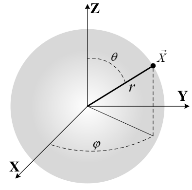
Assume that there exist plane-wave source signals where ’th source impinging in the angular direction with wave-number . The received signal at the ’th microphone from the ’th source at time is , where is the propagation delay of the ’th source between the reference and ’th microphone. For a narrow band sound source, the received signal can be written in this form:
| (1) |
where is the wave-vector corresponding to the ’th plane-wave. The received signal at ’th microphone at time is [19]:
| (2) |
where is the additive white Gaussian noise with zero mean and variance of the ’th microphone. The received signal in (2) can be restated in a matrix form as:
| (3) |
where , , , and is the direction matrix which is composed of the signal direction vectors as:
| (4) |
where
| (5) |
The ’th element of the is the incident sound field to the ’th microphone of the array from the ’th unit amplitude plane-wave. On the other hand, by solving the wave equation in the spherical coordinates [21], the following equality can be obtained:
| (6) |
where is the mode strength of order and it is defined for open sphere as:
| (7) |
and is the real-valued spherical harmonic of order and degree defined as:
| (8) |
In (7) and (8), , and are the spherical Bessel and Henkel functions, is the radius of the rigid sphere and is the associated Legendre polynomial of order and degree [22, 23]. Applying a proper truncation order [24] to (6), the sound field can be approximated inside a sphere of radius centered at the origin, as follows [11]:
| (9) |
where and is the Euler number. Rewriting (9) in the matrix form, we have:
| (10) |
where and is the source spherical harmonics matrix of size and defined as:
| (11) |
where
the array spherical harmonics matrix, , is the size of and defined similar to (11) and the mode strength matrix, , is the size of and defined as follows:
The spherical harmonics decomposition of the received signal can be obtained as[22, 21]:
| (12) |
where and are the coefficients of the spherical harmonics decomposition and denotes the entire surface area of the unit sphere. Since the number of microphones is limited, obtaining using (12) is not applicable; We do not access on the entire surface of the array. Actually the spherical microphone array (SMA) perform spatial sampling of using real-valued sampling weights, , corresponding to the ’th microphone [25, 26]:
| (13) |
Equation (13) can be represented as in a matrix form
| (14) |
where
Considering (13), the spherical harmonics are orthonormal as represented in [26]
| (15) |
where is identity matrix. Replacing (10) in (3) and multiplying both sides of the equation by and using equations (14) and (15), the received signal model in the SH domain can be calculated as:
| (16) |
where , and is the number of snapshots. is named higher-order ambisonic (HOA) signal [11] and is the noise vector in the SH domain. According to (16), the HOA signal is a linear instantaneous mixture of the sources signal. Transforming the received signals at the array to the SH domain is performed by applying the time domain encoding filter, , to the received signal of the array [24]. It must be noticed that the transformation filter, , is known for the given array.
III Deterministic Model for DOA Estimation
In this section, a new ML DOA estimation based on EM algorithm in the SH domain is proposed by considering unknown and deterministic sources. It is worth noting that the additive noise in (16) is spatially nonuniform white noise. Because the filter applied to is not an identity matrix. In the following, we investigate two cases of assumption for DOA estimation in the SH domain: i) uniform and ii) nonuniform noise.
III-A Uniform Noise
In this subsection, the deterministic ML DOA estimation for uniform noise case [27] is reviewed. The important formulas which have been employed in the subsequent sections are discussed.
Suppose that the additive noise vector to be zero mean Gaussian with the covariance matrix of . The set of unknown parameters are defined as , where . Thus, the likelihood function of the received signal in the SH domain will be:
| (17) |
where . Applying the logarithmic function to (17), the log-likelihood function will be obtained as:
| (18) |
Therefore, the ML estimator of can be formulated as:
| (19) |
In order to estimate , the ML estimator in (19) can be simplified as:
| (20) |
where .
Here and are the linear and non-linear parameters of our optimization problem,
respectively. Minimizing the objective function in (20) requires an exhaustive search in -dimension space.
To decrease the computational complexity of such joint optimization problems, an iterative process is proposed based on [28] as follows:
1) Initialize and find the optimal estimator of as:
| (21) |
where represents the pseudo inverse matrix.
2) Estimate by putting the optimal estimation of in the objective function as:
| (22) |
3) Estimate by considering the optimal estimation of obtained as (21).
4) Repeat steps 2 and 3 until the difference of the objective function between two iterations reaches a value lower than limit.
Algorithm 1 summarizes the iterative ML estimator under uniform noise case.
III-B Nonuniform Noise
Now let the noise vector be zero mean Gaussian with covariance matrix of . The set of unknown parameters are defined as . The likelihood function will be:
| (23) |
where . Thus, The log-likelihood function will be:
| (24) |
where
| (25) | ||||
| (26) | ||||
| (27) |
Therefore, the ML estimation of can be written as:
| (28) |
To solve the optimization problem of (28), an exhaustive search in -dimensional space is required. The iterative procedure mentioned in the previous subsection is employed to solve (28). In order to perform ML estimation of , we need to consider and alongside altogether. As a consequence, the sources’ signals and the variances must be estimated. Similar to the method introduced in III-A, first we fix and , and then estimate the noise variances as a function of and . By replacing the estimated noise variances in the objective function, the sources’ signals is estimated and DOAs are obtained. This procedure is explained in the following.
Equation (24) can be simplified to
| (29) |
where . The derivative of with respect to is calculated as:
| (30) |
Letting (30) to be zero, the ’th noise variances can be found:
| (31) |
where Substituting into (29), is simplified to:
| (32) |
Therefore, the ML estimator of and is given as:
| (33) |
Similar to the optimization problem of (20), can be presented as:
| (34) |
Substituting in (33), the ML estimator of is obtained as:
| (35) |
where and is defined similar to .
III-C Expectation Maximization Algorithm for deterministic ML DOA Estimation for spatially Nonuniform Noise
In this subsection, a new robust method based on EM algorithm is proposed for deterministic ML DOA estimation. The EM algorithm is an iterative method for obtaining ML estimation, where the data model includes both observed and unobserved latent variables. First, this approach is examined for a single source case and then it will be extended for multiple sources case.
III-C1 Single Source Case
As it can be seen in (16), the relationship between the received signal vector (incomplete data) and the complete data will be:
| (36) |
where is the HOA signal received from ’th source when only this source exists in the environment. According to (16), the received signal model in the SH domain can be stated as:
| (37) |
where is the Gaussian noise vector in the sole presence of the ’th source. Considering (28), the ML estimation will be
| (38) |
where and is defined in (24). and is ’th sound source signal and the covariance matrix of the noise vector, respectively. Similar to (31), can be estimated as:
| (39) |
where and . The deterministic ML estimation of single source DOA will be:
| (40) |
where
III-C2 Multiple Sources Case
The EM algorithm for deterministic ML DOA estimation is expanded for multiple sources in this part. Step by step procedure of the algorithm is explained as follows:
Initialization: Randomly initialize the direction of sources . The matrices and are initialized as follows:
| (41) |
Input to the ’th loop:
and .
Output of the ’th loop:
and .
Expectation step:
The noise covariance matrix is obtained from the single source case ones as:
| (42) |
The noise factor of the ’th single source, , is calculated as:
| (43) |
The HOA signal of each source can be estimated as:
| (44) |
where is obtained using (34).
Maximization step: The goal of this step is to find .
The vector can be obtained as a function of .
Then, is constructed:
| (45) | ||||
| (46) |
Note that is a function of . Therefore, the optimization problem to find will be:
| (47) |
After Estimating , the vector can be obtained. According to (39), the elements of the noise variance vector are estimated as:
| (48) |
| (49) |
Using the EM algorithm, the ML estimation of DOA of each source can be estimated separately. By comparing (47) with (35), it can be seen that the search space is reduced from -dimensional in (35) to 2-dimensional in (47). This improvement significantly decreases the optimization complexity.
The proposed EM algorithm for deterministic ML DOA estimation for nonuniform noise case is summarized in Algorithm 2.
| (50) |
IV Cramer-Rao Bound
In this section, CRB of the deterministic DOA estimator will be derived for a signal model with the spatially nonuniform noise. This work is the extension of [20] and [28] to the deterministic model of the sound sources in the SH domain.
Theorem 1.
CRB of the deterministic ML DOA estimator for spatially nonuniform noise in the SH domain is given by
| (51) | ||||
| (52) |
in which
| (53) | ||||
| (54) |
| (55) |
where and can be equal to or independently, is the covariance of the HOA signal, and
| (56) |
Proof.
See Appendix. ∎
V Simulation
In this section, the proposed EM algorithm is evaluated and compared with the traditional standard narrow-band MUSIC algorithm [5] and the recently proposed ICA based method [11] through various scenarios. In the conducted simulations, the SMA is an open array of radius 15 cm consisting 12 omnidirectional microphones. The SMA is located at the coordinates (5 m, 7 m, 1.5 m) of a room of size 8 m 10 m 3 m. Two sound sources are located at 2 m distance of the array at the angular locations of and . Configuration of the room and the position of the SMA and sources in the simulation setup are demonstrated in Fig. 2. The signal to reverberation ratio (SRR) is almost equal to -3.5 dB and the room reverberation time (RT60) is approximately 400 ms. The sources play the speech signals with duration about 1 s which are sampled at 16 KHz. The impulse response for the room between the sources and the SMA is calculated using MCRoomSim, which is a multichannel room acoustics simulator [29]. Microphone signals and additive white Gaussian noise are filtered with the HOA encoding filters which result in 2nd order HOA signals and SH domain noise, respectively. The length of the HOA encoding filters is 512 and designed such that its output SNR is maximized. Then, the HOA signals are filtered by bandpass filters with the pass-band of 500 to 3500 Hz. The optimization in (22) and (47) are performed by Nelder-Mead direct search method [30]. The FastlCA is used for applying the ICA algorithm in the MATLAB environment [31].

In Figs. 3 and 4, the average root mean square error (RMSE) of the estimating and for 50 different realizations in 30 dB SNR for EM, ICA, MUSIC, ML estimation for uniform noise case (see Alg. 1) and CRB versus the number of snapshots are presented. The MUSIC algorithm does not converge below 5000 snapshots. As the number of snapshots increase, the RMSE of estimation decreases for all DOA estimation methods. As expected, the EM algorithm outperforms the uniform noise case estimation, due to this fact that the nonuniform noise well matches the signal model in the SH domain.
The estimated and RMSE for the EM algorithm as a function of the SNR through boxplot representation is plotted in Figs. 5 and 6, respectively. In these figures, for each SNR value, the RMSE is obtained with the average of 50 different realizations of the proposed algorithm. The box has lines at the lower, median and upper quartile values of the RMSE. The whiskers are lines extending from each end of the box to show the extent of the rest of the values. Outliers are the values outside the ends of the whiskers. If there is no value outside the whisker, a dot is placed at the bottom whisker. As can be seen, SNR is increased by decreasing the RMSE variance. Therefore in higher SNR, the estimated value is likely closer to the true value.
The estimated and RMSE for EM, ICA, MUSIC, uniform ML estimation and CRB versus SNR is shown in Figs. 7 and 8, respectively. The range of SNR values is between 0 to 40 dB. The average of 50 different realizations is used to achieve each simulated point. As shown, the proposed algorithm is closer to the CRB compared to MUSIC and ICA. Performance of the ICA method is highly dropped in low SNR values due to not considering the environmental noise. In higher SNR values, the ICA assumption becomes closer to the reality, resulting in the ICA outperforms the MUSIC. The EM algorithm exhibits a better performance because of considering the environmental noise and reverberation. The signal is assumed to be independent and non-Gaussian for the ICA algorithm. But due to the reverberation, both assumptions are not realistic for DOA estimation. In order to show that the distribution of the HOA signal is Gaussian, Kolmogorov-Smirnov hypothesis test is used. The test result, with the 5% significance level, confirms that the HOA signals come from a Gaussian distribution. Also, the cross-correlation coefficient between the first and the second normalized HOA signals are calculated as which is equal to . For better visualization, the histogram of the second HOA signal and the cross-correlation between the first and second HOA signals are plotted in Figs. 9(a) and 9(b), respectively. Considering the signal model matches to the HOA domain, the EM algorithm can achieve lower RMSE for estimating and and is closer to the CRB. Referring to these results, we can say that the EM algorithm shows at least an improvement of 6 dB in robustness compared to the best of MUSIC and ICA methods in the noisy environments.
To examine the robustness of the EM algorithm in the reverberant environments, the average RMSE of the estimating and for EM, ICA and MUSIC for 50 different realizations in 40 dB SNR versus different RT60 are reported in Table I and II. In the lower RT60s, the ICA and EM algorithm almost have the same performance. Because the ICA method does not consider the correlation in the HOA signals, its RMSE grows by increasing the RT60. Also, the MUSIC algorithm shows an acceptable performance in the lower RT60 and degrades as RT60 increases. According to Tables II and I, the proposed algorithm demonstrates at least an improvement of 7 dB in robustness compared to the MUSIC and ICA methods in the reverberant environments as it was in the noisy environments.
| RT60 [sec] | EM | ICA | MUSIC |
|---|---|---|---|
| 0.110 | 0.183 | 0.186 | 0.893 |
| 0.241 | 0.249 | 0.502 | 0.998 |
| 0.301 | 0.290 | 0.870 | 1.564 |
| 0.411 | 0.344 | 1.469 | 2.379 |
| 0.650 | 0.386 | 1.877 | 2.500 |
| 0.799 | 0.410 | 2.198 | 2.834 |
| RT60 [sec] | EM | ICA | MUSIC |
|---|---|---|---|
| 0.110 | 0.192 | 0.218 | 1.001 |
| 0.241 | 0.263 | 0.701 | 1.404 |
| 0.301 | 0.291 | 1.000 | 1.500 |
| 0.411 | 0.320 | 2.691 | 1.579 |
| 0.650 | 0.396 | 2.740 | 1.681 |
| 0.799 | 0.457 | 2.488 | 2.623 |
VI Conclusion
In this paper, considering the general model of the received signal in the SH domain, the EM algorithm is proposed for deterministic ML estimation of DOA of multiple sources in the presence of spatially nonuniform noise. In order to reduce the complexity of the ML estimation, the algorithm is broken down into two expectation and maximization steps. In the expectation step, the HOA signal of each single source case (latent variable) is obtained from the observed HOA signal. In the maximization step, the DOA of each source is estimated using the corresponding HOA signal which is obtained in the expectation step. The simulation results demonstrated that the proposed algorithm shows at least 6 and 7 dB better robustness in terms of RMSE in the reverberant and noisy environments, respectively, compared to the MUSIC and ICA methods. Estimation of DOA through machine learning algorithms in the HOA domain is a part of our future work.
[Proof of Theorem 1] First, we define the unknown parameters vector as
| (57) |
According to the CRB theory, the variance of ’th entry of unbiased estimator satisfies the following inequality:
| (58) |
where the element of of Fisher information matrix is defined as:
| (59) |
and the density function of the observation will be
| (60) |
where and . After some mathematical manipulation, the derivative of the density function with respect to and can be simplified as follows:
| (61) | ||||
| (62) |
Therefore (59) can be rewritten as
| (63) |
where
| (64) |
The ’th column of is the function of . Thus, the derivative of respect to or yields a matrix with all zero elements except the ’th column. The derivative of matrix respect to and are defined as follows:
| (65) |
where the scalar derivatives and are respect to and , respectively. The reverse equation of (65) can be expressed as:
| (66) |
where the vector is the ’th column of the identity matrix . According to (57), the Fisher information matrix can be declared with the block matrix as follows:
| (67) |
where is a matrix and is obtained the same as (63) and the first and second derivatives are taken with respect to ’th and ’th entry of and , respectively. Using (63)-(66), can be simplified as
| (68) |
Eventually defining , the matrix will be:
| (69) |
where represents the Hadamard product and is defined for two matrices as:
| (70) |
It must be noted that matrices , and are similarly defined.
Considering the algebraic equality
| (71) |
where , , and are matrix and and . Consequently, the CRB of is found using (58):
| (72) | ||||
| (73) |
Acknowledgements
The authors would like to acknowledge Nicolas Epain and Andrew Wabnitz from CARLab, the university of Sydney, Australia for providing us the HOA and MCRoomSim toolbox.
References
- [1] H. Teutsch and W. Kellermann, “Detection and localization of multiple wideband acoustic sources based on wavefield decomposition using spherical apertures,” in IEEE International Conference on Acoustics, Speech and Signal Processing, Mar. 2008.
- [2] ——, “Estimation of the number of wideband sources in an acousticwave field using eigen-beam processing for circular apertures,” in IEEE Workshop on Applications of Signal Processing to Audio and Acoustics, 2005.
- [3] C. Blandin, A. Ozerov, and E. Vincent, “Multi-source TDOA estimation in reverberant audio using angular spectra and clustering,” Signal Processing, vol. 92, no. 8, pp. 1950–1960, Aug. 2012.
- [4] T. Tung, K. Yao, D. Chen, R. Hudson, and C. Reed, “Source localization and spatial filtering using wideband MUSIC and maximum power beamforming for multimedia applications,” in IEEE Workshop on Signal Processing Systems Design and Implementation, 1999.
- [5] R. Schmidt, “Multiple emitter location and signal parameter estimation,” IEEE Trans. Antennas and Propagation, vol. 34, no. 3, pp. 276–280, Mar. 1986.
- [6] R. Roy and T. Kailath, “ESPRIT-estimation of signal parameters via rotational invariance techniques,” IEEE Trans. Acoustics, Speech, and Signal Processing, vol. 37, no. 7, pp. 984–995, Jul. 1989.
- [7] R. Goossens and H. Rogier, “Unitary spherical ESPRIT: 2-d angle estimation with spherical arrays for scalar fields,” IET Signal Processing, vol. 3, no. 3, p. 221, 2009.
- [8] H. Sun, H. Teutsch, E. Mabande, and W. Kellermann, “Robust localization of multiple sources in reverberant environments using EB-ESPRIT with spherical microphone arrays,” in IEEE International Conference on Acoustics, Speech and Signal Processing (ICASSP), May 2011.
- [9] X. Li, S. Yan, X. Ma, and C. Hou, “Spherical harmonics MUSIC versus conventional MUSIC,” Applied Acoustics, vol. 72, no. 9, pp. 646–652, Sep. 2011.
- [10] L. Kumar, G. Bi, and R. M. Hegde, “The spherical harmonics root-music,” in IEEE International Conference on Acoustics, Speech and Signal Processing (ICASSP), Mar. 2016.
- [11] N. Epain and C. T. Jin, “Independent component analysis using spherical microphone arrays,” Acta Acustica united with Acustica, vol. 98, no. 1, pp. 91–102, Jan. 2012.
- [12] T. Noohi, N. Epain, and C. T. Jin, “Direction of arrival estimation for spherical microphone arrays by combination of independent component analysis and sparse recovery,” in IEEE International Conference on Acoustics, Speech and Signal Processing, May 2013.
- [13] ——, “Super-resolution acoustic imaging using sparse recovery with spatial priming,” in IEEE International Conference on Acoustics, Speech and Signal Processing (ICASSP), Apr. 2015.
- [14] C. T. Jin, N. Epain, and A. Parthy, “Design, optimization and evaluation of a dual-radius spherical microphone array,” IEEE/ACM Trans. Audio, Speech, and Language Processing, vol. 22, no. 1, pp. 193–204, Jan. 2014.
- [15] S. Tervo and A. Politis, “Direction of arrival estimation of reflections from room impulse responses using a spherical microphone array,” IEEE/ACM Trans. Audio, Speech, and Language Processing, vol. 23, no. 10, pp. 1539–1551, Oct. 2015.
- [16] A. Moore, C. Evers, and P. Naylor, “Direction of arrival estimation in the spherical harmonic domain using subspace pseudo-intensity vectors,” IEEE/ACM Trans. Audio, Speech, and Language Processing, pp. 1–1, 2016.
- [17] X. Pan, H. Wang, F. Wang, and C. Song, “Multiple spherical arrays design for acoustic source localization,” in Sensor Signal Processing for Defence (SSPD), Sep. 2016.
- [18] H. Sun, E. Mabande, K. Kowalczyk, and W. Kellermann, “Joint DOA and TDOA estimation for 3d localization of reflective surfaces using eigenbeam MVDR and spherical microphone arrays,” in IEEE International Conference on Acoustics, Speech and Signal Processing (ICASSP), May 2011.
- [19] H. Krim and M. Viberg, “Two decades of array signal processing research: the parametric approach,” IEEE Signal Process. Mag., vol. 13, no. 4, pp. 67–94, Jul. 1996.
- [20] L. Kumar and R. M. Hegde, “Stochastic cramer-rao bound analysis for DOA estimation in spherical harmonics domain,” IEEE Signal Processing Letters, vol. 22, no. 8, pp. 1030–1034, Aug. 2015.
- [21] E. G. Williams and J. A. Mann, “Fourier acoustics: Sound radiation and nearfield acoustical holography,” The Journal of the Acoustical Society of America, vol. 108, no. 4, pp. 1373–1373, Oct. 2000.
- [22] J. Driscoll and D. Healy, “Computing fourier transforms and convolutions on the 2-sphere,” Advances in Applied Mathematics, vol. 15, no. 2, pp. 202–250, Jun. 1994.
- [23] E. T. Whittaker and G. N. Watson, A Course of Modern Analysis. Cambridge University Press, 1996.
- [24] H. Sun, S. Yan, and U. P. Svensson, “Optimal higher order ambisonics encoding with predefined constraints,” IEEE Trans. Audio, Speech, and Language Processing, vol. 20, no. 3, pp. 742–754, Mar. 2012.
- [25] H. Chen, T. D. Abhayapala, and W. Zhang, “Theory and design of compact hybrid microphone arrays on two-dimensional planes for three-dimensional soundfield analysis,” The Journal of the Acoustical Society of America, vol. 138, no. 5, pp. 3081–3092, Nov. 2015.
- [26] B. Rafaely, “Analysis and design of spherical microphone arrays,” IEEE Trans. Speech and Audio Processing, vol. 13, no. 1, pp. 135–143, Jan. 2005.
- [27] J. Chen, R. Hudson, and K. Yao, “Maximum-likelihood source localization and unknown sensor location estimation for wideband signals in the near-field,” IEEE Trans. Signal Processing, vol. 50, no. 8, pp. 1843–1854, Aug. 2002.
- [28] C. Chen, F. Lorenzelli, R. Hudson, and K. Yao, “Maximum likelihood DOA estimation of multiple wideband sources in the presence of nonuniform sensor noise,” EURASIP Journal on Advances in Signal Processing, vol. 2008, no. 1, p. 835079, 2008.
- [29] A. Wabnitz, N. Epain, C. Jin, and A. Van Schaik, “Room acoustics simulation for multichannel microphone arrays,” in Proceedings of the International Symposium on Room Acoustics, 2010, pp. 1–6.
- [30] J. C. Lagarias, J. A. Reeds, M. H. Wright, and P. E. Wright, “Convergence properties of the nelder–mead simplex method in low dimensions,” SIAM Journal on Optimization, vol. 9, no. 1, pp. 112–147, Jan. 1998.
- [31] H. Gavert, J. Hurri, J. Sarela, and A. Hyvarinen. The fastica package for matlab. [Online]. Available: https://research.ics.aalto.fi/ica/fastica/