Wider and Deeper, Cheaper and Faster:
Tensorized LSTMs for Sequence Learning

It can be seen from (2) that in an RNN, the parameter number scales quadratically with the size of the hidden state. A popular way to limit the parameter number when widening the network is to organize parameters as higher-dimensional tensors which can be factorized into lower-rank sub-tensors that contain significantly fewer elements [47, 46, 15, 26, 39, 51, 6, 18, 32], which is is known as tensor factorization. This implicitly widens the network since the hidden state vectors are in fact broadcast to interact with the tensorized parameters. Another common way to reduce the parameter number is to share a small set of parameters across different locations in the hidden state, similar to Convolutional Neural Networks (CNNs) [34, 35].

We adopt parameter sharing to cutdown the parameter number for RNNs, since compared with factorization, it has the following advantages: (i) scalability, i.e., the number of shared parameters can be set independent of the hidden state size, and (ii) separability, i.e., the information flow can be carefully managed by controlling the receptive field, allowing one to shift RNN deep computations to the temporal domain (see Sec. 2.2). We also explicitly tensorize the RNN hidden state vectors, since compared with vectors, tensors have a better: (i) flexibility, i.e., one can specify which dimensions to share parameters and then can just increase the size of those dimensions without introducing additional parameters, and (ii) efficiency, i.e., with higher-dimensional tensors, the network can be widened faster w.r.t. its depth when fixing the parameter number (see Sec. 2.3).

For ease of exposition, we first consider 2D tensors (matrices): we tensorize the hidden state $\bm{h}_{t}\!\in\!\mathbb{R}^{M}$ to become $\bm{H}_{t}\!\in\!\mathbb{R}^{P\!\times\!M}$, where $P$ is the tensor size, and $M$ the channel size. We locally-connect the first dimension of $\bm{H}_{t}$ in order to share parameters, and fully-connect the second dimension of $\bm{H}_{t}$ to allow global interactions. This is analogous to the CNN which fully-connects one dimension (e.g., the RGB channel for input images) to globally fuse different feature planes. Also, if one compares $\bm{H}_{t}$ to the hidden state of a Stacked RNN (sRNN) (see Fig. 1(a)), then $P$ is akin to the number of stacked hidden layers, and $M$ the size of each hidden layer. We start to describe our model based on 2D tensors, and finally show how to strengthen the model with higher-dimensional tensors.

Since an RNN is already deep in its temporal direction, we can deepen an input-to-output computation by associating the input $\bm{x}_{t}$ with a (delayed) future output. In doing this, we need to ensure that the output $\bm{y}_{t}$ is separable, i.e., not influenced by any future input $\bm{x}_{t^{\prime}}$ ($t^{\prime}\!>\!t$). Thus, we concatenate the projection of $\bm{x}_{t}$ to the top of the previous hidden state $\bm{H}_{t-1}$, then gradually shift the input information down when the temporal computation proceeds, and finally generate $\bm{y}_{t}$ from the bottom of $\bm{H}_{t+L-1}$, where $L\!-\!1$ is the number of delayed timesteps for computations of depth $L$. An example with $L\!=\!3$ is shown in Fig. 1(b). This is in fact a skewed sRNN as used in [1] (also similar to [48]). However, our method does not need to change the network structure and also allows different kinds of interactions as long as the output is separable, e.g, one can increase the local connections and use feedback (see Fig. 1(c)), which can be beneficial for sRNNs [10]. In order to share parameters, we update $\bm{H}_{t}$ using a convolution with a learnable kernel. In this manner we increase the complexity of the input-to-output mapping (by delaying outputs) and limit parameter growth (by sharing transition parameters using convolutions).

To describe the resulting tRNN model, let $\bm{H}^{cat}_{t-1}\!\in\!\mathbb{R}^{(P+1)\!\times\!M}$ be the concatenated hidden state, and $p\!\in\!\mathbb{Z}_{+}$ the location at a tensor. The channel vector $\bm{h}^{cat}_{t-1,p}\!\in\!\mathbb{R}^{M}$ at location $p$ of $\bm{H}^{cat}_{t-1}$ is defined as:

where $\bm{W}^{x}\in\mathbb{R}^{R\!\times\!M}$ and $\bm{b}^{x}\in\mathbb{R}^{M}$. Then, the update of tensor $\bm{H}_{t}$ is implemented via a convolution:

where $\bm{W}^{h}\!\in\!\mathbb{R}^{K\!\times\!M^{i}\!\times\!M^{o}}$ is the kernel weight of size $K$, with $M^{i}\!=\!M$ input channels and $M^{o}\!=\!M$ output channels, $\bm{b}^{h}\!\in\!\mathbb{R}^{M^{o}}$ is the kernel bias, $\bm{A}_{t}\!\in\!\mathbb{R}^{P\!\times\!M^{o}}$ is the hidden activation, and $\circledast$ is the convolution operator (see Appendix A.1 for a more detailed definition). Since the kernel convolves across different hidden layers, we call it the cross-layer convolution. The kernel enables interaction, both bottom-up and top-down across layers. Finally, we generate $\bm{y}_{t}$ from the channel vector $\bm{h}_{t+L-1,P}\!\in\!\mathbb{R}^{M}$ which is located at the bottom of $\bm{H}_{t+L-1}$:

where $\bm{W}^{y}\!\in\!\mathbb{R}^{M\!\times\!S}$ and $\bm{b}^{y}\!\in\!\mathbb{R}^{S}$. To guarantee that the receptive field of $\bm{y}_{t}$ only covers the current and previous inputs $\bm{x}_{1:t}$ (see Fig. 1(c)), $L$, $P$, and $K$ should satisfy the constraint:

where $\lceil\cdot\rceil$ is the ceil operation. For the derivation of (9), please see Appendix B.

We call the model defined in (5)-(8) the Tensorized RNN (tRNN). The model can be widened by increasing the tensor size $P$, whilst the parameter number remains fixed (thanks to the convolution). Also, unlike the sRNN of runtime complexity $O(TL)$, tRNN breaks down the runtime complexity to $O(T\!+\!L)$, which means either increasing the sequence length $T$ or the network depth $L$ would not significantly increase the runtime.

To allow the tRNN to capture long-range temporal dependencies, one can straightforwardly extend it to an LSTM by replacing the tRNN tensor update equations of (6)-(7) as follows:

where the kernel $\{\bm{W}^{h},\bm{b}^{h}\}$ is of size $K$, with $M^{i}\!\!=\!\!M$ input channels and $M^{o}\!\!=\!4M$ output channels, $\bm{A}^{g}_{t},\!\bm{A}^{i}_{t},\!\bm{A}^{f}_{t},\!\bm{A}^{o}_{t}\!\in\!\mathbb{R}^{P\!\times\!M}$ are activations for the new content $\bm{G}_{t}$, input gate $\bm{I}_{t}$, forget gate $\bm{F}_{t}$, and output gate $\bm{O}_{t}$, respectively, $\sigma(\cdot)$ is the element-wise sigmoid function, and $\bm{C}_{t}\!\in\!\mathbb{R}^{P\!\times\!M}$ is the memory cell. However, since in (12) the previous memory cell $\bm{C}_{t-1}$ is only gated along the temporal direction (see Fig. 1(d)), long-range dependencies from the input to output might be lost when the tensor size $P$ becomes large.

Memory Cell Convolution.    To capture long-range dependencies from multiple directions, we additionally introduce a novel memory cell convolution, by which the memory cells can have a larger receptive field (see Fig. 1(e)). We also dynamically generate this convolution kernel so that it is both time- and location-dependent, allowing for flexible control over long-range dependencies from different directions. This results in our tLSTM tensor update equations:

where, in contrast to (10)-(13), the kernel $\{\bm{W}^{h},\bm{b}^{h}\}$ has additional $\langle K\rangle$ output channels²² 2 The operator $\langle\cdot\rangle$ returns the cumulative product of all elements in the input variable. to generate the activation $\bm{A}^{q}_{t}\!\in\!\mathbb{R}^{P\!\times\!\langle\!K\!\rangle}$ for the dynamic kernel bank $\bm{Q}_{t}\!\in\!\mathbb{R}^{P\!\times\!\langle\!K\!\rangle}$, $\bm{q}_{t,p}\!\in\!\mathbb{R}^{\langle\!K\!\rangle}$ is the vectorized adaptive kernel at the location $p$ of $\bm{Q}_{t}$, and $\bm{W}^{c}_{t}(p)\!\in\!\mathbb{R}^{K\!\times 1\times 1}$ is the dynamic kernel of size $K$ with a single input/output channel, which is reshaped from $\bm{q}_{t,p}$ (see Fig. 2(a) for an illustration). In (17), each channel of the previous memory cell $\bm{C}_{t-1}$ is convolved with $\bm{W}^{c}_{t}(p)$ whose values vary with $p$, forming a memory cell convolution (see Appendix A.2 for a more detailed definition), which produces a convolved memory cell $\bm{C}^{conv}_{t-1}\!\in\!\mathbb{R}^{P\!\times\!M}$. Note that in (15) we employ a softmax function $\varsigma(\cdot)$ to normalize the channel dimension of $\bm{Q}_{t}$, which, similar to [37], can stabilize the value of memory cells and help to prevent the vanishing/exploding gradients (see Appendix C for details).

The idea of dynamically generating network weights has been used in many works [44, 46, 15, 6, 14, 23], where in [14] location-dependent convolutional kernels are also dynamically generated to improve CNNs. In contrast to these works, we focus on broadening the receptive field of tLSTM memory cells. Whilst the flexibility is retained, fewer parameters are required to generate the kernel since the kernel is shared by different memory cell channels.

Channel Normalization.    To improve training, we adapt Layer Normalization (LN) [3] to our tLSTM. Similar to the observation in [3] that LN does not work well in CNNs where channel vectors at different locations have very different statistics, we find that LN is also unsuitable for tLSTM where lower level information is near the input while higher level information is near the output. We therefore normalize the channel vectors at different locations with their own statistics, forming a Channel Normalization (CN), with its operator $\operatorname{CN}\left(\cdot\right)$:

where $\bm{Z},\widehat{\bm{Z}},\bm{\Gamma},\bm{B}\in\mathbb{R}^{P\times M^{z}}$ are the original tensor, normalized tensor, gain parameter, and bias parameter, respectively. The $m^{z}$-th channel of $\bm{Z}$, i.e. $\bm{z}_{m^{z}}\!\in\!\mathbb{R}^{P}$, is normalized element-wisely:

where $\bm{z}^{\mu},\bm{z}^{\sigma}\!\in\!\mathbb{R}^{P}$ are the mean and standard deviation along the channel dimension of $\bm{Z}$, respectively, and $\widehat{\bm{z}}_{m^{z}}\!\in\!\mathbb{R}^{P}$ is the $m^{z}$-th channel of $\widehat{\bm{Z}}$. Note that the number of parameters introduced by CN/LN can be neglected as it is very small compared to the number of other parameters in the model.

Using Higher-Dimensional Tensors.    One can observe from (9) that when fixing the kernel size $K$, the tensor size $P$ of a 2D tLSTM grows linearly w.r.t. its depth $L$. How can we expand the tensor volume more rapidly so that the network can be widened more efficiently? We can achieve this goal by leveraging higher-dimensional tensors. Based on previous definitions for 2D tLSTMs, we replace the 2D tensors with $D$-dimensional ($D\!>\!2$) tensors, obtaining $\bm{H}_{t},\bm{C}_{t}\!\in\!\mathbb{R}^{P_{1}\!\times\!P_{2}\!\times\!\ldots\!\times\!P_{D\!-\!1}\!\times\!M}$ with the tensor size $\textit{{P}}\!=\!\left[P_{1},P_{2},\ldots,P_{D-1}\right]$. Since the hidden states are no longer matrices, we concatenate the projection of $\bm{x}_{t}$ to one corner of $\bm{H}_{t-1}$, and thus (5) is extended as:

where $\bm{h}^{cat}_{t-1,\bm{p}}\!\in\!\mathbb{R}^{M}$ is the channel vector at location $\bm{p}\!\in\!\mathbb{Z}^{D-1}_{+}$ of the concatenated hidden state $\bm{H}^{cat}_{t-1}\!\in\!\mathbb{R}^{(\!P_{1}+1\!)\!\times\!(\!P_{2}+1\!)\!\times\!\ldots\!\times\!(\!P_{D\!-\!1}+1\!)\!\times\!M}$. For the tensor update, the convolution kernel $\bm{W}^{h}$ and $\bm{W}^{c}_{t}(\cdot)$ also increase their dimensionality with kernel size $\textit{{K}}=\left[K_{1},K_{2},\ldots,K_{D-1}\right]$. Note that $\bm{W}^{c}_{t}(\cdot)$ is reshaped from the vector, as illustrated in Fig. 2(b). Correspondingly, we generate the output $\bm{y}_{t}$ from the opposite corner of $\bm{H}_{t+L-1}$, and therefore (8) is modified as:

For convenience, we set $P_{d}=P$ and $K_{d}=K$ for $d=1,2,\ldots,D-1$ so that all dimensions of P and K can satisfy (9) with the same depth $L$. In addition, CN still normalizes the channel dimension of tensors.

The Hutter Prize Wikipedia dataset [25] consists of 100 million characters taken from 205 different characters including alphabets, XML markups and special symbols. We model the dataset at the character-level, and try to predict the next character of the input sequence.

We fix the parameter number to 10M, corresponding to channel sizes $M$ of 1120 for sLSTM and 2D tLSTM–F, 901 for other 2D tLSTMs, and 522 for 3D tLSTMs. All configurations are evaluated with depths $L\!=\!1,2,3,4$. We use Bits-per-character (BPC) to measure the model performance.

Results are shown in Fig. 3. When $L\!\leq\!2$, sLSTM and 2D tLSTM–F outperform other models because of a larger $M$. With $L$ increasing, the performances of sLSTM and 2D tLSTM–M improve but become saturated when $L\!\geq\!3$, while tLSTMs with memory cell convolutions improve with increasing $L$ and finally outperform both sLSTM and 2D tLSTM–M. When $L\!=\!4$, 2D tLSTM–F is surpassed by 2D tLSTM, which is in turn surpassed by 3D tLSTM. The performance of 3D tLSTM+LN benefits from LN only when $L\!\leq\!2$. However, 3D tLSTM+CN consistently improves 3D tLSTM with different $L$.

Whilst the runtime of sLSTM is almost proportional to $L$, it is nearly constant in each tLSTM configuration and largely independent of $L$.

We compare a larger model, i.e. a 3D tLSTM+CN with $L\!=\!6$ and $M\!=\!1200$, to the state-of-the-art methods on the test set, as reported in Table 1. Our model achieves 1.264 BPC with 50.1M parameters, and is competitive to the best performing methods [54, 38] with similar parameter numbers.

(a) Addition: The task is to sum two 15-digit integers. The network first reads two integers with one digit per timestep, and then predicts the summation. We follow the processing of [30], where a symbol ‘-’ is used to delimit the integers as well as pad the input/target sequence. A 3-digit integer addition task is of the form:

(b) Memorization: The goal of this task is to memorize a sequence of 20 random symbols. Similar to the addition task, we use 65 different symbols. A 5-symbol memorization task is of the form:

We evaluate all configurations with $L\!=\!1,4,7,10$ on both tasks, where $M$ is 400 for addition and 100 for memorization. The performance is measured by the symbol prediction accuracy.

Fig. 4 show the results. In both tasks, large $L$ degrades the performances of sLSTM and 2D tLSTM–M. In contrast, the performance of 2D tLSTM–F steadily improves with $L$ increasing, and is further enhanced by using feedback connections, higher-dimensional tensors, and CN, while LN helps only when $L\!=\!1$. Note that in both tasks, the correct solution can be found (when $100\%$ test accuracy is achieved) due to the repetitive nature of the task. In our experiment, we also observe that for the addition task, 3D tLSTM+CN with $L\!=\!7$ outperforms other configurations and finds the solution with only 298K training samples, while for the memorization task, 3D tLSTM+CN with $L\!=\!10$ beats others configurations and achieves perfect memorization after seeing 54K training samples. Also, unlike in sLSTM, the runtime of all tLSTMs is largely unaffected by $L$.

We further compare the best performing configurations to the state-of-the-art methods for both tasks (see Table 2). Our models solve both tasks significantly faster (i.e., using fewer training samples) than other models, achieving the new state-of-the-art results.

The MNIST dataset [35] consists of 50000/10000/10000 handwritten digit images of size $28\!\times\!28$ for training/validation/test. We have two tasks on this dataset:

(a) Sequential MNIST: The goal is to classify the digit after sequentially reading the pixels in a scanline order [33]. It is therefore a 784 timestep sequence learning task where a single output is produced at the last timestep; the task requires very long range dependencies in the sequence.

(b) Sequential Permuted MNIST: We permute the original image pixels in a fixed random order as in [2], resulting in a permuted MNIST (pMNIST) problem that has even longer range dependencies across pixels and is harder.

In both tasks, all configurations are evaluated with $M\!=\!100$ and $L\!=\!1,3,5$. The model performance is measured by the classification accuracy.

Results are shown in Fig. 5. sLSTM and 2D tLSTM–M no longer benefit from the increased depth when $L\!=\!5$. Both increasing the depth and tensorization boost the performance of 2D tLSTM. However, removing feedback connections from 2D tLSTM seems not to affect the performance. On the other hand, CN enhances the 3D tLSTM and when $L\!\geq\!3$ it outperforms LN. 3D tLSTM+CN with $L\!=\!5$ achieves the highest performances in both tasks, with a validation accuracy of 99.1% for MNIST and 95.6% for pMNIST. The runtime of tLSTMs is negligibly affected by $L$, and all tLSTMs become faster than sLSTM when $L\!=\!5$.

We also compare the configurations of the highest test accuracies to the state-of-the-art methods (see Table 3). For sequential MNIST, our 3D tLSTM+CN with $L\!=\!3$ performs as well as the state-of-the-art Dilated GRU model [8], with a test accuracy of 99.2%. For the sequential pMNIST, our 3D tLSTM+CN with $L\!=\!5$ has a test accuracy of 95.7%, which is close to the state-of-the-art of 96.7% produced by the Dilated CNN [40] in [8].

The experimental results of different model configurations on different tasks suggest that the performance of tLSTMs can be improved by increasing the tensor size and network depth, requiring no additional parameters and little additional runtime. As the network gets wider and deeper, we found that the memory cell convolution mechanism is crucial to maintain improvement in performance. Also, we found that feedback connections are useful for tasks of sequential output (e.g., our Wikipedia and algorithmic tasks). Moreover, tLSTM can be further strengthened via tensorization or CN.

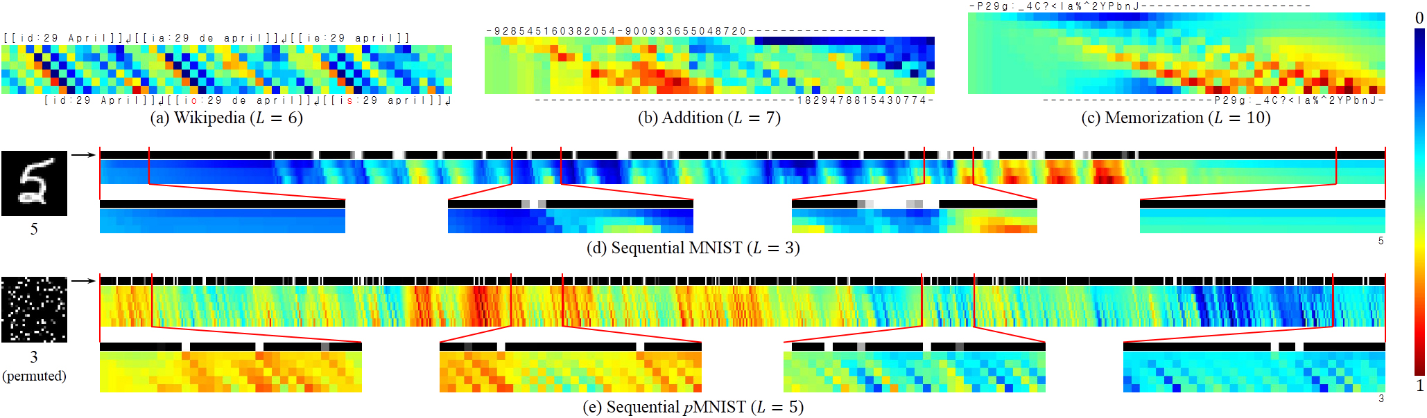
It is also intriguing to examine the internal working mechanism of tLSTM. Thus, we visualize the memory cell which gives insight into how information is routed. For each task, the best performing tLSTM is run on a random example. We record the channel mean (the mean over channels, e.g., it is of size $P\!\times\!P$ for 3D tLSTMs) of the memory cell at each timestep, and visualize the diagonal values of the channel mean from location $\bm{p}^{in}\!=\![1,1]$ (near the input) to $\bm{p}^{out}\!=\![P,P]$ (near the output).

Visualization results in Fig. 6 reveal the distinct behaviors of tLSTM when dealing with different tasks: (i) Wikipedia: the input can be carried to the output location with less modification if it is sufficient to determine the next character, and vice versa; (ii) addition: the first integer is gradually encoded into memories and then interacts (performs addition) with the second integer, producing the sum; (iii) memorization: the network behaves like a shift register that continues to move the input symbol to the output location at the correct timestep; (iv) sequential MNIST: the network is more sensitive to the pixel value change (representing the contour, or topology of the digit) and can gradually accumulate evidence for the final prediction; (v) sequential pMNIST: the network is sensitive to high value pixels (representing the foreground digit), and we conjecture that this is because the permutation destroys the topology of the digit, making each high value pixel potentially important.

From Fig. 6 we can also observe common phenomena for all tasks: (i) at each timestep, the values at different tensor locations are markedly different, implying that wider (larger) tensors can encode more information, with less effort to compress it; (ii) from the input to the output, the values become increasingly distinct and are shifted by time, revealing that deep computations are indeed performed together with temporal computations, with long-range dependencies carried by memory cells.

References

- [1] Jeremy Appleyard, Tomas Kocisky, and Phil Blunsom. Optimizing performance of recurrent neural networks on gpus. arXiv preprint arXiv:1604.01946, 2016.
- [2] Martin Arjovsky, Amar Shah, and Yoshua Bengio. Unitary evolution recurrent neural networks. In ICML, 2016.
- [3] Jimmy Lei Ba, Jamie Ryan Kiros, and Geoffrey E Hinton. Layer normalization. arXiv preprint arXiv:1607.06450, 2016.
- [4] Yoshua Bengio, Patrice Simard, and Paolo Frasconi. Learning long-term dependencies with gradient descent is difficult. IEEE TNN, 5(2):157–166, 1994.
- [5] Yoshua Bengio. Learning deep architectures for ai. Foundations and trends® in Machine Learning, 2009.
- [6] Luca Bertinetto, João F Henriques, Jack Valmadre, Philip Torr, and Andrea Vedaldi. Learning feed-forward one-shot learners. In NIPS, 2016.
- [7] James Bradbury, Stephen Merity, Caiming Xiong, and Richard Socher. Quasi-recurrent neural networks. In ICLR, 2017.
- [8] Shiyu Chang, Yang Zhang, Wei Han, Mo Yu, Xiaoxiao Guo, Wei Tan, Xiaodong Cui, Michael Witbrock, Mark Hasegawa-Johnson, and Thomas Huang. Dilated recurrent neural networks. In NIPS, 2017.
- [9] Jianxu Chen, Lin Yang, Yizhe Zhang, Mark Alber, and Danny Z Chen. Combining fully convolutional and recurrent neural networks for 3d biomedical image segmentation. In NIPS, 2016.
- [10] Junyoung Chung, Caglar Gulcehre, Kyunghyun Cho, and Yoshua Bengio. Gated feedback recurrent neural networks. In ICML, 2015.
- [11] Junyoung Chung, Sungjin Ahn, and Yoshua Bengio. Hierarchical multiscale recurrent neural networks. In ICLR, 2017.
- [12] Ronan Collobert, Koray Kavukcuoglu, and Clément Farabet. Torch7: A matlab-like environment for machine learning. In NIPS Workshop, 2011.
- [13] Tim Cooijmans, Nicolas Ballas, César Laurent, and Aaron Courville. Recurrent batch normalization. In ICLR, 2017.
- [14] Bert De Brabandere, Xu Jia, Tinne Tuytelaars, and Luc Van Gool. Dynamic filter networks. In NIPS, 2016.
- [15] Misha Denil, Babak Shakibi, Laurent Dinh, Nando de Freitas, et al. Predicting parameters in deep learning. In NIPS, 2013.
- [16] Greg Diamos, Shubho Sengupta, Bryan Catanzaro, Mike Chrzanowski, Adam Coates, Erich Elsen, Jesse Engel, Awni Hannun, and Sanjeev Satheesh. Persistent rnns: Stashing recurrent weights on-chip. In ICML, 2016.
- [17] Jeffrey L Elman. Finding structure in time. Cognitive science, 14(2):179–211, 1990.
- [18] Timur Garipov, Dmitry Podoprikhin, Alexander Novikov, and Dmitry Vetrov. Ultimate tensorization: compressing convolutional and fc layers alike. In NIPS Workshop, 2016.
- [19] Felix A Gers, Jürgen Schmidhuber, and Fred Cummins. Learning to forget: Continual prediction with lstm. Neural computation, 12(10):2451–2471, 2000.
- [20] Alex Graves, Abdel-rahman Mohamed, and Geoffrey Hinton. Speech recognition with deep recurrent neural networks. In ICASSP, 2013.
- [21] Alex Graves. Generating sequences with recurrent neural networks. arXiv preprint arXiv:1308.0850, 2013.
- [22] Alex Graves. Adaptive computation time for recurrent neural networks. arXiv preprint arXiv:1603.08983, 2016.
- [23] David Ha, Andrew Dai, and Quoc V Le. Hypernetworks. In ICLR, 2017.
- [24] Sepp Hochreiter and Jürgen Schmidhuber. Long short-term memory. Neural computation, 9(8):1735–1780, 1997.
- [25] Marcus Hutter. The human knowledge compression contest. URL http://prize.hutter1.net, 2012.
- [26] Ozan Irsoy and Claire Cardie. Modeling compositionality with multiplicative recurrent neural networks. In ICLR, 2015.
- [27] Rafal Jozefowicz, Wojciech Zaremba, and Ilya Sutskever. An empirical exploration of recurrent network architectures. In ICML, 2015.
- [28] Łukasz Kaiser and Samy Bengio. Can active memory replace attention? In NIPS, 2016.
- [29] Łukasz Kaiser and Ilya Sutskever. Neural gpus learn algorithms. In ICLR, 2016.
- [30] Nal Kalchbrenner, Ivo Danihelka, and Alex Graves. Grid long short-term memory. In ICLR, 2016.
- [31] Diederik Kingma and Jimmy Ba. Adam: A method for stochastic optimization. In ICLR, 2015.
- [32] Ben Krause, Liang Lu, Iain Murray, and Steve Renals. Multiplicative lstm for sequence modelling. In ICLR Workshop, 2017.
- [33] Quoc V Le, Navdeep Jaitly, and Geoffrey E Hinton. A simple way to initialize recurrent networks of rectified linear units. arXiv preprint arXiv:1504.00941, 2015.
- [34] Yann LeCun, Bernhard Boser, John S Denker, Donnie Henderson, Richard E Howard, Wayne Hubbard, and Lawrence D Jackel. Backpropagation applied to handwritten zip code recognition. Neural computation, 1(4):541–551, 1989.
- [35] Yann LeCun, Léon Bottou, Yoshua Bengio, and Patrick Haffner. Gradient-based learning applied to document recognition. Proceedings of the IEEE, 86(11):2278–2324, 1998.
- [36] Tao Lei and Yu Zhang. Training rnns as fast as cnns. arXiv preprint arXiv:1709.02755, 2017.
- [37] Gundram Leifert, Tobias Strauß, Tobias Grüning, Welf Wustlich, and Roger Labahn. Cells in multidimensional recurrent neural networks. JMLR, 17(1):3313–3349, 2016.
- [38] Asier Mujika, Florian Meier, and Angelika Steger. Fast-slow recurrent neural networks. In NIPS, 2017.
- [39] Alexander Novikov, Dmitrii Podoprikhin, Anton Osokin, and Dmitry P Vetrov. Tensorizing neural networks. In NIPS, 2015.
- [40] Aaron van den Oord, Sander Dieleman, Heiga Zen, Karen Simonyan, Oriol Vinyals, Alex Graves, Nal Kalchbrenner, Andrew Senior, and Koray Kavukcuoglu. Wavenet: A generative model for raw audio. arXiv preprint arXiv:1609.03499, 2016.
- [41] Viorica Patraucean, Ankur Handa, and Roberto Cipolla. Spatio-temporal video autoencoder with differentiable memory. In ICLR Workshop, 2016.
- [42] Bernardino Romera-Paredes and Philip Hilaire Sean Torr. Recurrent instance segmentation. In ECCV, 2016.
- [43] David E Rumelhart, Geoffrey E Hinton, and Ronald J Williams. Learning representations by back-propagating errors. Nature, 323(6088):533–536, 1986.
- [44] Jürgen Schmidhuber. Learning to control fast-weight memories: An alternative to dynamic recurrent networks. Neural Computation, 4(1):131–139, 1992.
- [45] Marijn F Stollenga, Wonmin Byeon, Marcus Liwicki, and Juergen Schmidhuber. Parallel multi-dimensional lstm, with application to fast biomedical volumetric image segmentation. In NIPS, 2015.
- [46] Ilya Sutskever, James Martens, and Geoffrey E Hinton. Generating text with recurrent neural networks. In ICML, 2011.
- [47] Graham W Taylor and Geoffrey E Hinton. Factored conditional restricted boltzmann machines for modeling motion style. In ICML, 2009.
- [48] Aaron van den Oord, Nal Kalchbrenner, and Koray Kavukcuoglu. Pixel recurrent neural networks. In ICML, 2016.
- [49] Scott Wisdom, Thomas Powers, John Hershey, Jonathan Le Roux, and Les Atlas. Full-capacity unitary recurrent neural networks. In NIPS, 2016.
- [50] Lin Wu, Chunhua Shen, and Anton van den Hengel. Deep recurrent convolutional networks for video-based person re-identification: An end-to-end approach. arXiv preprint arXiv:1606.01609, 2016.
- [51] Yuhuai Wu, Saizheng Zhang, Ying Zhang, Yoshua Bengio, and Ruslan Salakhutdinov. On multiplicative integration with recurrent neural networks. In NIPS, 2016.
- [52] SHI Xingjian, Zhourong Chen, Hao Wang, Dit-Yan Yeung, Wai-kin Wong, and Wang-chun Woo. Convolutional lstm network: A machine learning approach for precipitation nowcasting. In NIPS, 2015.
- [53] Saizheng Zhang, Yuhuai Wu, Tong Che, Zhouhan Lin, Roland Memisevic, Ruslan R Salakhutdinov, and Yoshua Bengio. Architectural complexity measures of recurrent neural networks. In NIPS, 2016.
- [54] Julian Georg Zilly, Rupesh Kumar Srivastava, Jan Koutník, and Jürgen Schmidhuber. Recurrent highway networks. In ICML, 2017.
Appendix A Mathematical Definition for Cross-Layer Convolutions
A.1 Hidden State Convolution
The hidden state convolution in (6) is defined as: