Practical Data-Dependent Metric Compression
with Provable Guarantees
Abstract
We introduce a new distance-preserving compact representation of multi-dimensional point-sets. Given points in a -dimensional space where each coordinate is represented using bits (i.e., bits per point), it produces a representation of size bits per point from which one can approximate the distances up to a factor of . Our algorithm almost matches the recent bound of [IW17] while being much simpler. We compare our algorithm to Product Quantization (PQ) [JDS11], a state of the art heuristic metric compression method. We evaluate both algorithms on several data sets: SIFT (used in [JDS11]), MNIST [LC98], New York City taxi time series [GMRS16] and a synthetic one-dimensional data set embedded in a high-dimensional space. With appropriately tuned parameters, our algorithm produces representations that are comparable to or better than those produced by PQ, while having provable guarantees on its performance.
1 Introduction
Compact distance-preserving representations of high-dimensional objects are very useful tools in data analysis and machine learning. They compress each data point in a data set using a small number of bits while preserving the distances between the points up to a controllable accuracy. This makes it possible to run data analysis algorithms, such as similarity search, machine learning classifiers, etc, on data sets of reduced size. The benefits of this approach include: (a) reduced running time (b) reduced storage and (c) reduced communication cost (between machines, between CPU and RAM, between CPU and GPU, etc). These three factors make the computation more efficient overall, especially on modern architectures where the communication cost is often the dominant factor in the running time, so fitting the data in a single processing unit is highly beneficial. Because of these benefits, various compact representations have been extensively studied over the last decade, for applications such as: speeding up similarity search [Bro97, IM98, KOR00, TFW08, WTF09, JDS11, NFS12, SL14], scalable learning algorithms [WDL+09, LSMK11], streaming algorithms [M+05] and other tasks. For example, a recent paper [JDJ17] describes a similarity search software package based on one such method (Product Quantization (PQ)) that has been used to solve very large similarity search problems over billions of point on GPUs at Facebook.
The methods for designing such representations can be classified into data-dependent and data-oblivious. The former analyze the whole data set in order to construct the point-set representation, while the latter apply a fixed procedure individually to each data point. A classic example of the data-oblivious approach is based on randomized dimensionality reduction [JL84], which states that any set of points in the Euclidean space of arbitrary dimension can be mapped into a space of dimension , such that the distances between all pairs of points are preserved up to a factor of . This allows representing each point using bits, where is the number of bits of precision in the coordinates of the original pointset. 11 1 The bounds can be stated more generally in terms of the aspect ratio of the point-set. See Section 2 for the discussion. More efficient representations are possible if the goal is to preserve only the distances in a certain range. In particular, bits are sufficient to distinguish between distances smaller than and greater than , independently of the precision parameter [KOR00] (see also [RL09] for kernel generalizations). Even more efficient methods are known if the coordinates are binary [Bro97, LSMK11, SL14].
Data-dependent methods compute the bit representations of points “holistically", typically by solving a global optimization problem. Examples of this approach include Semantic Hashing [SH09], Spectral Hashing [WTF09] or Product Quantization [JDS11] (see also the survey [WLKC16]). Although successful, most of the results in this line of research are empirical in nature, and we are not aware of any worst-case accuracy vs. compression tradeoff bounds for those methods along the lines of the aforementioned data oblivious approaches.
A recent work [IW17] shows that it is possible to combine the two approaches and obtain algorithms that adapt to the data while providing worst-case accuracy/compression tradeoffs. In particular, the latter paper shows how to construct representations of -dimensional pointsets that preserve all distances up to a factor of while using only bits per point. Their algorithm uses hierarchical clustering in order to group close points together, and represents each point by a displacement vector from a near by point that has already been stored. The displacement vector is then appropriately rounded to reduce the representation size. Although theoretically interesting, that algorithm is rather complex and (to the best of our knowledge) has not been implemented.
Our results.
The main contribution of this paper is QuadSketch (QS), a simple data-adaptive algorithm, which is both provable and practical. It represents each point using bits, where (as before) we can set using the Johnson-Lindenstrauss lemma. Our bound significantly improves over the “vanilla” bound (obtained by storing all coordinates to full precision), and comes close to bound of [IW17]. At the same time, the algorithm is quite simple and intuitive: it computes a -dimensional quadtree22 2 Traditionally, the term “quadtree” is used for the case of , while its higher-dimensional variants are called “ hyperoctrees” [YS83]. However, for the sake of simplicity, in this paper we use the same term “quadtree” for any value of . and appropriately prunes its edges and nodes.33 3 We note that a similar idea (using kd-trees instead of quadtrees) has been earlier proposed in [AZ14]. However, we are not aware of any provable space/distortion tradeoffs for the latter algorithm.
We evaluate QuadSketch experimentally on both real and synthetic data sets: a SIFT feature data set from [JDS11], MNIST [LC98], time series data reflecting taxi ridership in New York City [GMRS16] and a synthetic data set (Diagonal) containing random points from a one-dimensional subspace (i.e., a line) embedded in a high-dimensional space. The data sets are quite diverse: SIFT and MNIST data sets are de-facto “standard” test cases for nearest neighbor search and distance preserving sketches, NYC taxi data was designed to contain anomalies and “irrelevant” dimensions, while Diagonal has extremely low intrinsic dimension. We compare our algorithms to Product Quantization (PQ) [JDS11], a state of the art method for computing distance-preserving sketches, as well as a baseline simple uniform quantization method (Grid). The sketch length/accuracy tradeoffs for QS and PQ are comparable on SIFT and MNIST data, with PQ having higher accuracy for shorter sketches while QS having better accuracy for longer sketches. On NYC taxi data, the accuracy of QS is higher over the whole range of sketch lengths . Finally, Diagonal exemplifies a situation where the low dimensionality of the data set hinders the performance of PQ, while QS naturally adapts to this data set. Overall, QS performs well on “typical” data sets, while its provable guarantees ensure robust performance in a wide range of scenarios. Both algorithms improve over the baseline quantization method.
2 Formal Statement of Results
Preliminaries.
Let be a pointset in Euclidean space. A compression scheme constructs from a bit representation referred to as a sketch. Given the sketch, and without access to the original pointset, one can decompress the sketch into an approximate pointset . The goal is to minimize the size of the sketch, while approximately preserving the geometric properties of the pointset, in particular the distances and near neighbors.
In the previous section we parameterized the sketch size in terms of the number of points , the dimension , and the bits per coordinate . In fact, our results are more general, and can be stated in terms of the aspect ratio of the pointset, denoted by and defined as the ratio between the largest to smallest distance,
Note that , so our bounds, stated in terms of , immediately imply analogous bounds in terms of .
We will use to denote , and to suppress polylogarithmic factors in .
QuadSketch.
Our compression algorithm, described in detail in Section 3, is based on a randomized variant of a quadtree followed by a pruning step. In its simplest variant, the trade-off between the sketch size and compression quality is governed by a single parameter . Specifically, controls the pruning step, in which the algorithm identifies “non-important” bits among those stored in the quadtree (i.e. bits whose omission would have little effect on the approximation quality), and removes them from the sketch. Higher values of result in sketches that are longer but have better approximation quality.
Approximate nearest neighbors.
Our main theorem provides the following guarantees for the basic variant of QuadSketch: for each point, the distances from that point to all other points are preserved up to a factor of with a constant probability.
Theorem 1.
Given , let and . QuadSketch runs in time and produces a sketch of size bits, with the following guarantee: For every ,
In particular, with probability , if is the nearest neighbor of in , then is a -approximate nearest neighbor of in .
Note that the theorem allows us to compress the input point-set into a sketch and then decompress it back into a point-set which can be fed to a black box similarity search algorithm. Alternatively, one can decompress only specific points and approximate the distance between them.
For example, if and is polynomially bounded in , then Theorem 1 uses bits per coordinate to preserve -approximate nearest neighbors.
Maximum distortion.
We also show that a recursive application of QuadSketch makes it possible to approximately preserve the distances between all pairs of points. This is the setting considered in [IW17]. (In contrast, Theorem 1 preserves the distances from any single point.)
Theorem 2.
Given , let and . There is a randomized algorithm that runs in time and produces a sketch of size bits, such that with high probability, every distance can be recovered from the sketch up to distortion .
Theorem 2 has smaller sketch size than that provided by the “vanilla” bound, and only slightly larger than that in [IW17]. For example, for and , it improves over the “vanilla” bound by a factor of and is lossier than the bound of [IW17] by a factor of . However, compared to the latter, our construction time is nearly linear in . The comparison is summarized in Table 1.
3 The Compression Scheme
The sketching algorithm takes as input the pointset , and two parameters and that control the amount of compression.
Step 1: Randomly shifted grid.
The algorithm starts by imposing a randomly shifted axis-parallel grid on the points. We first enclose the whole pointset in an axis-parallel hypercube . Let , and . Set up to be centered at with side length . Now choose independently and uniformly at random, and shift in each coordinate by . By the choice of side length , one can see that after the shift still contains the whole pointset. For every integer such that , let denote the axis-parallel grid with cell side which is aligned with .
Note that this step can be often eliminated in practice without affecting the empirical performance of the algorithm, but it is necessary in order to achieve guarantees for arbitrary pointsets.
Step 2: Quadtree construction.
The -ary quadtree on the nested grids is naturally defined by associating every grid cell in with the tree node at level , such that its children are the grid cells in which are contained in . The edge connecting a node to a child is labeled with a bitstring of length defined as follows: the bit is if coincides with the bottom half of along coordinate , and if coincides with the upper half along that coordinate.
In order to construct the tree, we start with as the root, and bucket the points contained in it into the children cells. We only add child nodes for cells that contain at least one point of . Then we continue by recursing on the child nodes. The quadtree construction is finished after levels. We denote the resulting edge-labeled tree by . A construction for is illustrated in Figure 1.
We define the level of a tree node with side length to be (note that can be negative). The degree of a node in is its number of children. Since all leaves are located at the bottom level, each point is contained in exactly one leaf, which we henceforth denote by .
Step 3: Pruning.
Consider a downward path in , such that are nodes with degree , and are nodes with degree other than ( may be a leaf). For every such path in , if , we remove the nodes from with all their adjacent edges (and edge labels). Instead we connect directly to as its child. We refer to that edge as the long edge, and label it with the length of the path it replaces (). The original edges from are called short edges. At the end of the pruning step, we denote the resulting tree by .
The sketch.
For each point the sketch stores the index of the leaf that contains it. In addition it stores the structure of the tree , encoded using the Eulerian Tour Technique44 4 See e.g., https://en.wikipedia.org/wiki/Euler_tour_technique.. Specifically, starting at the root, we traverse in the Depth First Search (DFS) order. In each step, DFS either explores the child of the current node (downward step), or returns to the parent node (upward step). We encode a downward step by and an upward step by . With each downward step we also store the label of the traversed edge (a length- bitstring for a short edge or the edge length for a long edge, and an additional bit marking if the edge is short or long).
Decompression.
Recovering from the sketch is done simply by following the downward path from the root of to the associated leaf , collecting the edge labels of the short edges, and placing zeros instead of the missing bits of the long edges. The collected bits then correspond to the binary expansion of the coordinates of .
More formally, for every node (not necessarily a leaf) we define as follows: For , concatenate the bit of every short edge label traversed along the downward path from the root to . When traversing a long edge labeled with length , concatenate zeros.55 5 This is the “lossy” step in our sketching method: the original bits could be arbitrary, but they are replaced with zeros. Then, place a binary floating point in the resulting bitstring, after the bit corresponding to level . (Recall that the levels in are defined by the grid cell side lengths, and might not have any nodes in level ; in this case we need to pad with ’s either on the right or on the left until we have a bit in the location corresponding to level .) The resulting binary string is the binary expansion of the coordinate of . Now is defined to be .
Block QuadSketch.
We can further modify QuadSketch in a manner similar to Product Quantization [JDS11]. Specifically, we partition the dimensions into blocks of size each, and apply QuadSketch separately to each block. More formally, for each , we apply QuadSketch to the pointset , where denotes the -dimensional vector obtained by projecting on the dimensions in .
The following statement is an immediate corollary of Theorem 1.
Theorem 3.
Given , and dividing , set the pruning parameter to and the number of levels to . The -block variant of QuadSketch runs in time and produces a sketch of size bits, with the following guarantee: For every ,
It can be seen that increasing the number of blocks up to a certain threshold ( ) does not affect the asymptotic bound on the sketch size. Although we cannot prove that varying allows to improve the accuracy of the sketch, this seems to be the case empirically, as demonstrated in the experimental section.
4 Experiments
We evaluate QuadSketch experimentally and compare its performance to Product Quantization (PQ) [JDS11], a state-of-the-art compression scheme for approximate nearest neighbors, and to a baseline of uniform scalar quantization, which we refer to as Grid. For each dimension of the dataset, Grid places equally spaced landmark scalars on the interval between the minimum and the maximum values along that dimension, and rounds each coordinate to the nearest landmark.
All three algorithms work by partitioning the data dimensions into blocks, and performing a quantization step in each block independently of the other ones. QuadSketch and PQ take the number of blocks as a parameter, and Grid uses blocks of size . The quantization step is the basic algorithm described in Section 3 for QuadSketch, -means for PQ, and uniform scalar quantization for Grid.
We test the algorithms on four datasets: The SIFT data used in [JDS11], MNIST [LC98] (with all vectors normalized to ), NYC Taxi ridership data [GMRS16], and a synthetic dataset called Diagonal, consisting of random points on a line embedded in a high-dimensional space. The properties of the datasets are summarized in Table 2. Note that we were not able to compute the exact diameters for MNIST and SIFT, hence we only report estimates for for these data sets, obtained via random sampling.
The Diagonal dataset consists of points of the form , where is chosen independently and uniformly at random from the interval . This yields a dataset with a very large aspect ratio , and on which partitioning into blocks is not expected to be beneficial since all coordinates are maximally correlated.
For SIFT and MNIST we use the standard query set provided with each dataset. For Taxi and Diagonal we use queries chosen at random from each dataset. For the sake of consistency, for all data sets, we apply the same quantization process jointly to both the point set and the query set, for both PQ and QS. We note, however, that both algorithms can be run on “out of sample” queries.
| Dataset | Points | Dimension | Aspect ratio () |
|---|---|---|---|
| SIFT | |||
| MNIST | |||
| NYC Taxi | |||
| Diagonal (synthetic) |
For each dataset, we enumerate the number of blocks over all divisors of the dimension . For QuadSketch, ranges in , and ranges in . For PQ, the number of -means landmarks per block ranges in . For both algorithms we include the results for all combinations of the parameters, and plot the envelope of the best performing combinations.
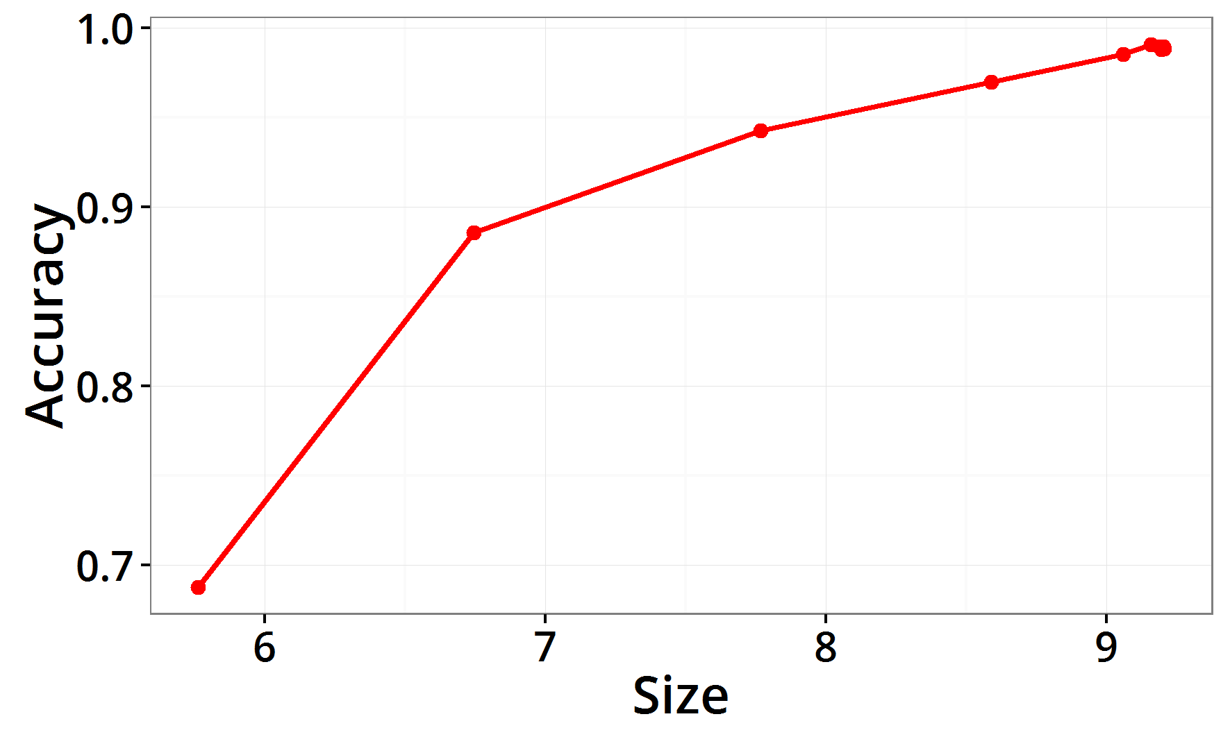
We report two measures of performance for each dataset: (a) the accuracy, defined as the fraction of queries for which the sketch returns the true nearest neighbor, and (b) the average distortion, defined as the ratio between the (true) distances from the query to the reported near neighbor and to the true nearest neighbor. The sketch size is measured in bits per coordinate. The results appear in Figures 5, 5, 5 and 5. Note that the vertical coordinate in the distortion plots corresponds to the value of , not .


4.1 QuadSketch Parameter Setting
We plot how the different parameters of QuadSketch effect its performance. Recall that determines the number of levels in the quadtree prior to the pruning step, and controls the amount of pruning. By construction, the higher we set these parameters, the larger the sketch will be and with better accuracy. The empirical tradeoff for the SIFT dataset is plotted in Figure 7.

The optimal setting for the number of blocks is not monotone, and generally depends on the specific dataset. It was noted in [JDS11] that on SIFT data an intermediate number of blocks gives the best results, and this is confirmed by our experiments. Table 3 lists the performance on the SIFT dataset for a varying number of blocks, for a fixed setting of and . It shows that the sketch quality remains essentially the same, while the size varies significantly, with the optimal size attained at blocks.
| # Blocks | Bits per coordinate | Accuracy | Average distortion |
|---|---|---|---|
5 Proofs
In this section we prove Theorems 1 and 2. Recall that we have a pointset with aspect ratio , and given error parameters . For the remainder of the section we fix the setting
Recall that in Section 3 we let denote the grid with side length for every integer . Our analysis is based on the observation that randomly shifting the grids, which is used as the first step of our algorithm, induces a padded decomposition [Bar96] of the pointset. We now define this formally.
Definition 1 (padded point).
We say that a point is -padded, if the grid cell in that contains also contains the ball of radius centered at , where
We say that is -padded in the quadtree , if it is -padded for every level of .
Note that and are fixed parameters for a given input. We omit their dependence from the notation for simplicity.
We now prove Theorem 1. It follows directly from combining the following two lemmas.
Lemma 1.
If the grids are randomly shifted, as in Section 3, then every point is -padded in with probability .
Proof.
Fix a point , a coordinate and a level . Let denote the value of in coordinate . Along this coordinate, we are randomly shifting a -dimensional grid partitioned into intervals of length . Since the shift is uniformly random, the probability for to be at distance at most from an endpoint of the interval that contains it equals . By plugging our setting of and , this probability equals . Taking a union bound over the coordinates, we have probability at most for to be at distance at most from the boundary of the cell of that contains it. In the complement event is -padded in . Taking another union bound over the levels in the quadtree, is -padded with probability at least . ∎
Lemma 2.
Proof.
We recall that is a pruned quadtree in which every node is associated with a grid cell of an axis-parallel grid with side length , which is aligned with and contained in . We call the level of , and denote it henceforth by . We will use the term “bottom-left corner” of a grid cell for the corner that minimizes all coordinate values (i.e., the high-dimensional analog of a bottom-left corner in the plane).
Let be the root of . We may assume w.l.o.g. that the bottom-left corner of is the origin in , since translating together with the entire pointset does not change pairwise distances. Under this assumption, we make the following observation, illustrated in Figure 8.
Observation 1.
Let be a node in . If the path from to contains only short edges, then (defined by the decompression algorithm in Section 3) is the bottom-left corner of the grid cell associated with .
Let be a padded point, and be any point. Recall that we denote by and the leaves corresponding to and respectively (see Section 3). Let be the lowest common ancestor of and in . Since and are in separate grid cells of , and the cell containing also contains the ball of radius around , we have
| (1) |
Let be the lowest node on the downward path from to , that can be reached without traversing a long edge. Similarly define for . See Figure 9 for illustration.
Note that must be either the leaf , or an internal node whose only outgoing edge is a long edge. In both cases, is the bottom of a path of degree- nodes of length :
- •
If is a leaf: Since the pointset has aspect ratio , then after levels the grid becomes sufficiently fine such that each grid cell contains at most one point . Since we generate the quadtree with levels, then each point is in its own grid cell for at least the bottom levels of the quadtree.
- •
If is an internal node which is the head of a long edge: Since the pruning step only places long edges at the bottom of degree- paths of length , then must be the bottom node of such path.
On the other hand is an ancestor of , and it has degree at least , since it is also an ancestor of . Hence is at least levels above , implying . Applying the same arguments to we get also .

Let be the bottom-left corners of the grid cells associated with and . If all edges on the downward paths from the root of to and were short, then Observation 1 would yield that and . In general, there might be some long edges on those paths, but they all must lie on the subpath from the root of down to , which is the same for both paths. This is because by the choice of and , all downward edges from to either of them are short. Therefore and are shifted from the true bottom-left corners by the same shift, which we denote by
Next, observe that the grid cell associated with has side and it contains both and . Therefore .
Furthermore, since is an ancestor of , then by the definition of and , in each coordinate, the binary expansions of these two vertices are equal from the location and up. In the less significant locations, is zeroed while may have arbitrary bits. This means that the difference between and in each coordinate can be at most in the absolute value, and consequently . Recalling that the decompression algorithm defines , we get .
Collecting the above inequalities, we have
Similarly for we have . Together, by the triangle inequality,
To complete the proof of Lemma 2 it remains to show , which follows from Equation 1. ∎
5.1 Sketch Size and Running Time
Lemma 3.
QuadSketch produces a sketch of size bits.
Proof.
The tree has leaves, and we have pruned each non-branching path in it to length . Hence its total size is , and its structure can be stored with this many bits using (for example) the DFS scan described in Section 3. Each short edge label is bits long, so together they consume bits. As for the long edges, there can be at most of them, since the bottom of each long edge is either a branching node or a leaf. The long edge labels are lengths of downward paths in the non-pruned tree , whose height bounded by is . Together the long edge labels consume bits, which is dominated by . Finally for each point we store the index of its corresponding leaf , and since there are leaves, this requires additional bits to store. ∎
Lemma 4.
The QuadSketch construction algorithm runs in time .
Proof.
Given a quadtree cell and a point contained in it, in order to bucket the point into a cell in the next level, we need to check for each coordinate whether the point falls in the upper or lower half of the cell. This takes time . Since each point is bucketed once in every level, and we generate for levels, the quadtree construction time is . The pruning step requires just a linear scan of , in time . ∎
5.2 Maximum Distortion
We now prove Theorem 2.
Sketching algorithm
Given a pointset , apply QuadSketch to and let be the resulting tree. Let be the padded points in (meaning those for which the condition of Lemma 1 is satisfied for ). Continue by recursion on , until all points in are padded in some tree. The returned sketch contains all trees constructed during the recursion, and in addition, for every point we store the index of the tree in which it is padded.
Query algorithm
Given two point indices , assume w.l.o.g. , then the tree has corresponding leaves for both and . We decompress and from and return .
Analysis
The correctness of the estimate up to distortion follows from Lemma 2. We now bound the sketch size and the running time. Lemma 1 with implies that in each of the trees , the expected fraction of padded points is . Hence by Markov’s inequality, with probability at least half the points are padded. Since the calls to QuadSketch are independent (and its success probability depends only on its internal randomness and not on the input points), with probability this happens in each of the first iterations. This probability can be amplified to constant by independent repetitions. If this event has happened then the sketching algorithm terminates since becomes empty. Therefore the total running time of a successful execution is calls to QuadSketch, which by Lemma 4 is .
Furthermore, since the number of padded points decreases by at least half in every iteration, the total size of the sketches is
the same as in Theorem 1 up to a constant factor. Finally, since each is index in , the ’s only take additional bits to store. ∎
Acknowledgements
This research was supported by grants from NSF, Simons Foundation, and Shell (via MIT Energy Initiative).
References
- [AZ14] Relja Arandjelović and Andrew Zisserman, Extremely low bit-rate nearest neighbor search using a set compression tree, IEEE transactions on pattern analysis and machine intelligence 36 (2014), no. 12, 2396–2406.
- [Bar96] Yair Bartal, Probabilistic approximation of metric spaces and its algorithmic applications, Foundations of Computer Science, 1996. Proceedings., 37th Annual Symposium on, IEEE, 1996, pp. 184–193.
- [Bro97] Andrei Z Broder, On the resemblance and containment of documents, Compression and Complexity of Sequences 1997. Proceedings, IEEE, 1997, pp. 21–29.
- [GMRS16] Sudipto Guha, Nina Mishra, Gourav Roy, and Okke Schrijvers, Robust random cut forest based anomaly detection on streams, International Conference on Machine Learning, 2016, pp. 2712–2721.
- [IM98] Piotr Indyk and Rajeev Motwani, Approximate nearest neighbors: towards removing the curse of dimensionality, Proceedings of the thirtieth annual ACM symposium on Theory of computing, ACM, 1998, pp. 604–613.
- [IW17] Piotr Indyk and Tal Wagner, Near-optimal (euclidean) metric compression, Proceedings of the Twenty-Eighth Annual ACM-SIAM Symposium on Discrete Algorithms, SIAM, 2017, pp. 710–723.
- [JDJ17] Jeff Johnson, Matthijs Douze, and Hervé Jégou, Billion-scale similarity search with gpus, CoRR abs/1702.08734 (2017).
- [JDS11] Herve Jegou, Matthijs Douze, and Cordelia Schmid, Product quantization for nearest neighbor search, IEEE transactions on pattern analysis and machine intelligence 33 (2011), no. 1, 117–128.
- [JL84] William B Johnson and Joram Lindenstrauss, Extensions of lipschitz mappings into a hilbert space, Contemporary mathematics 26 (1984), no. 189-206, 1.
- [KOR00] Eyal Kushilevitz, Rafail Ostrovsky, and Yuval Rabani, Efficient search for approximate nearest neighbor in high dimensional spaces, SIAM Journal on Computing 30 (2000), no. 2, 457–474.
- [LC98] Yann LeCun and Corinna Cortes, The mnist database of handwritten digits, 1998.
- [LSMK11] Ping Li, Anshumali Shrivastava, Joshua L Moore, and Arnd C König, Hashing algorithms for large-scale learning, Advances in neural information processing systems, 2011, pp. 2672–2680.
- [M+05] Shanmugavelayutham Muthukrishnan et al., Data streams: Algorithms and applications, Foundations and Trends® in Theoretical Computer Science 1 (2005), no. 2, 117–236.
- [NF13] Mohammad Norouzi and David J Fleet, Cartesian k-means, Proceedings of the IEEE Conference on Computer Vision and Pattern Recognition, 2013, pp. 3017–3024.
- [NFS12] Mohammad Norouzi, David J Fleet, and Ruslan R Salakhutdinov, Hamming distance metric learning, Advances in neural information processing systems, 2012, pp. 1061–1069.
- [RL09] Maxim Raginsky and Svetlana Lazebnik, Locality-sensitive binary codes from shift-invariant kernels, Advances in neural information processing systems, 2009, pp. 1509–1517.
- [SH09] Ruslan Salakhutdinov and Geoffrey Hinton, Semantic hashing, International Journal of Approximate Reasoning 50 (2009), no. 7, 969–978.
- [SL14] Anshumali Shrivastava and Ping Li, Densifying one permutation hashing via rotation for fast near neighbor search., ICML, 2014, pp. 557–565.
- [TFW08] Antonio Torralba, Rob Fergus, and Yair Weiss, Small codes and large image databases for recognition, Computer Vision and Pattern Recognition, 2008. CVPR 2008. IEEE Conference on, IEEE, 2008, pp. 1–8.
- [WDL+09] Kilian Weinberger, Anirban Dasgupta, John Langford, Alex Smola, and Josh Attenberg, Feature hashing for large scale multitask learning, Proceedings of the 26th Annual International Conference on Machine Learning, ACM, 2009, pp. 1113–1120.
- [WLKC16] Jun Wang, Wei Liu, Sanjiv Kumar, and Shih-Fu Chang, Learning to hash for indexing big data: a survey, Proceedings of the IEEE 104 (2016), no. 1, 34–57.
- [WTF09] Yair Weiss, Antonio Torralba, and Rob Fergus, Spectral hashing, Advances in neural information processing systems, 2009, pp. 1753–1760.
- [YS83] Mann-May Yau and Sargur N Srihari, A hierarchical data structure for multidimensional digital images, Communications of the ACM 26 (1983), no. 7, 504–515.