Localization of Multiple Targets with Identical Radar Signatures in Multipath Environments with Correlated Blocking
Abstract
This paper addresses the problem of localizing an unknown number of targets, all having the same radar signature, by a distributed MIMO radar consisting of single antenna transmitters and receivers that cannot determine directions of departure and arrival. Furthermore, we consider the presence of multipath propagation, and the possible (correlated) blocking of the direct paths (going from the transmitter and reflecting off a target to the receiver). In its most general form, this problem can be cast as a Bayesian estimation problem where every multipath component is accounted for. However, when the environment map is unknown, this problem is ill-posed and hence, a tractable approximation is derived where only direct paths are accounted for. In particular, we take into account the correlated blocking by scatterers in the environment which appears as a prior term in the Bayesian estimation framework. A sub-optimal polynomial-time algorithm to solve the Bayesian multi-target localization problem with correlated blocking is proposed and its performance is evaluated using simulations. We found that when correlated blocking is severe, assuming the blocking events to be independent and having constant probability (as was done in previous papers) resulted in poor detection performance, with false alarms more likely to occur than detections.
Index Terms:
Multi-target localization, Correlated blocking, distributed MIMO radar, data association, matchingI Introduction
Over the past decade, there has been an increasing demand for accurate indoor localization solutions to support a multitude of applications, ranging from providing location-based advertising to users in a shopping mall [1], to better solutions for tracking inventory in a warehouse [2], to assisted-living applications [3]. In many of these applications, the availability of location information enhances communication protocols (e.g., in a warehouse, communication with a tag can take place once it is within range of a reader) and the importance of localization to such communications systems has led to standardization efforts such as IEEE 802.15.4a [4], which is a standard for joint localization and communication. While localization of cellular devices falls under the category of active localization (where the target transmits a ranging signal), the current paper will focus on the important case of passive localization, where the target only reflects radio-frequency (RF) signals (i.e., radar). In the above-mentioned applications, there are usually multiple targets present that have nearly identical radar signatures and hence, cannot be distinguished on that basis alone.
The typical localization architecture involves the deployment of multiple transmitters (TXs) and receivers (RXs) and hence, can be modeled using the distributed MIMO (multiple-input multiple-output) radar framework [5]. Due to cost and space constraints (e.g., in sensor applications), each TX and RX may be equipped with a single antenna only11 1 Since a major contributor to the cost is the amplifier in a RF chain, a cheaper distributed MIMO architecture can be realized by deploying a single RF chain each for the TX and RX antennas and switching between them.. Hence, the radar cannot exploit the information contained in the angles of arrival/departure from the target-reflected signal as direction finding requires not just multiple antennas, but also careful calibration of the antenna elements, which might be cost-prohibitive in the case of sensor nodes and similar devices. This motivates the study of multi-target localization (MTL) without angular information in an indoor distributed MIMO radar setting.
In such a setting, a direct path (DP) is one that propagates directly from TX to target to RX. Each DP gives rise to an ellipse-shaped ambiguity region passing through the target location, with the TX and RX at the foci, and the intersection of three or more such curves unambiguously determine the target location. For indoor localization, the following additional challenges arise - (i) targets can be blocked by non-target scatterers such as walls, furniture etc., (ii) the scatterers can also give rise to indirect paths (IPs) which need to be distinguished from DPs, (iii) in the presence of multiple targets, yet another challenge is to match the DPs to the right targets22 2 This process is also referred to as data association [6, 7]. Throughout this work, we shall use the term matching to refer to data association.. An incorrect matching would result in ghost targets [8].
There has been a considerable amount of literature on MIMO radar over the last decade. The fundamental limits of localization in MIMO radar networks were studied in [9]. A number of works have dealt with MTL using co-located antenna arrays at the TX and RX [10, 11, 12, 13, 14, 15, 16, 17, 18, 19, 20, 21, 22]. The single-target localization problem using widely-spaced antenna arrays was investigated in [23, 24] and the multi-target case in [25]. None of these works address the issues of blocking and multipath common in an indoor environment. The works closest to ours are [26] and [8], where MTL in a distributed MIMO radar setting is addressed. The experiments and the system model in [26] do not consider the effect of blocking and a brute-force method is used for matching the DPs to targets, which is computationally infeasible for a large number of targets, as shown in Section IV. On the other hand,[8] considers the effect of blocking, but relies on the assumption of a constant and independent blocking probability for all DPs. In reality however, the DP blocking events in any environment are not mutually independent. As shown in Fig. 1, the location of the two TXs is such that if one of them has line-of-sight (LoS) to the target, it is highly likely that the other does as well. Similarly, if one of them is blocked with respect to the target, it is highly likely that the other is as well. In other words, the DP blocking events are, in general, correlated and the extent of correlation depends on the network geometry. In this work, we investigate how correlated blocking can be exploited to obtain better location estimates for the targets.

Intuitively, our approach works as follows: when three or more ellipses intersect at a point, we first assume that they are DPs. We then compute the joint probability that LoS exists to the TXs and RXs in question at the point of intersection. If the probability is sufficiently high, then we conclude that a target is present.
The main contributions of this work are as follows:
- •
The general problem of localizing all targets and scatterers in an unknown environment is cast as a Bayesian estimation problem. Such a fundamental formulation of the problem goes beyond the description in [8] (and other papers, to the best of our knowledge).
- •
We show this problem to be ill-posed and proceed to derive a tractable approximation called the Bayesian MTL problem, where the objective is to localize only the targets, but not the scatterers. This is also a Bayesian estimation problem where the joint DP blocking distribution plays the role of a prior.
- •
We propose a polynomial time approximate algorithm to solve the Bayesian MTL problem, which can be used even when only empirical blocking statistics, obtained via measurements or simulations, are available.
This paper consists of six sections. In the system model in Section II, we define decision variables to decide if a multipath component (MPC) is a DP, IP or a noise peak. The generalized problem of localizing all targets and scatterers is formulated as a Bayesian estimation problem in Section III, where along with the target and scatterer locations, the aforementioned decision variables are the estimation parameters. Furthermore, this problem is shown to be ill-posed and a more tractable approximation called the Bayesian MTL problem is derived, where the objective is to localize only the targets. In Section IV, the brute force solution to the Bayesian MTL problem is shown to have exponential complexity in the number of targets and TX-RX pairs (TRPs). As a result, a sub-optimal polynomial time algorithm taking correlated blocking into account is proposed instead. Simulation as well as experimental results for the proposed algorithm are presented in Section V and finally, Section VI concludes the paper.
Notation: Vectors and scalars are represented using bold (e.g., ) and regular (e.g., ) lowercase letters, respectively. In particular, denotes the all-one vector. For a collection of scalars , where and are discrete index sets, denotes the column vector containing all , ordered first according to index , followed by and so on. Similarly, and respectively denote summation and product over index , followed by and so on. For positive integers and , denotes the modulo operator, i.e., the remainder of the operation . The set of real numbers is denoted by . For , denotes the greatest integer lesser than or equal to . For continuous random variables and , denotes their joint probability density function (pdf), the marginal pdf of , and the conditional pdf of , given . and denote the probability and expectation operators, respectively.
II System Model
In this section, we introduce the formal notation to decide the identity of a MPC and model the correlated blocking of DPs. This lays the groundwork for the fundamental problem formulation that will then be solved in Sections III and IV.
Consider a distributed MIMO radar with TXs and RXs, each equipped with a single omni-directional antenna and deployed in an unknown environment. An unknown number of stationary point targets33 3 The point target assumption simplifies the analysis of the problem, as each target can give rise to at most one DP. The impact of real (i.e., non-point) targets can be seen in our experimental results, presented in Section V-D. are present and the objective is to localize all of them. We assume that the environment has non-target scatterers too, which can either block some target(s) to some TX(s) and/or RX(s), and/or give rise to IPs. All TX and RX locations are assumed to be known. The number of TRPs, denoted by , equals . Unless otherwise mentioned, the convention throughout this work is that the -th TRP comprises of the -th TX and -th RX, where and (Table I).
| TRP No. | 1 | 2 | 3 | 4 | 5 | 6 | 7 | 8 | 9 |
| TX No. | 1 | 2 | 3 | 1 | 2 | 3 | 1 | 2 | 3 |
| RX No. | 1 | 1 | 1 | 2 | 2 | 2 | 3 | 3 | 3 |
For ease of notation, we restrict our attention to the two-dimensional (2D) case, where all the TXs, RXs, scatterers and targets are assumed to lie in the horizontal plane. The extension to the 3D case is straightforward. Let the TX and the RX for the -th TRP be located at and , respectively. We assume that the TXs use orthogonal signals so that the RXs can distinguish between signals sent from different TXs. For each TRP, the RX extracts the channel impulse response from the measured receive signal; an MPC is assumed to exist at a particular delay (within the resolution limit of the RX) when the amplitude of the impulse response at that delay bin exceeds a threshold; alternately, a maximum likelihood (ML) estimator or other high-resolution algorithms can be used to extract the amplitudes and delays of all the MPCs [27],[28]. All MPCs that do not involve a reflection off a target (e.g., TXscattererRX) are assumed to be removed by a background cancellation technique. For stationary or even slow-moving targets, a simple way to achieve this is to measure the impulse responses for all the TRPs when no targets are present. This set of template signals can then be subtracted from the signals obtained when the target(s) are introduced, which would remove MPCs of the form TXscattererRX since they appear twice [29]. Other background subtraction techniques for localization and tracking applications are described in [30],[31]. An MPC involving more than two reflections is assumed to be too weak to be detected. Finally, two or more MPCs could have their delays so close to one another that they can be unresolvable due to finite bandwidth. Under this model, each extracted MPC could be one or more of the following:
- 1.
A DP to one or more targets, which occurs when a target has LoS to both the TX and RX in question.
- 2.
An IP of the first kind, which is of the form TXtargetscattererRX.
- 3.
An IP of the second kind, having the form TXscatterertargetRX.
- 4.
A noise peak.
Each MPC gives rise to a time-of-arrival (ToA) estimate which, in turn, corresponds to a range estimate. If only additive white Gaussian noise (AWGN) is present at the RXs, then each ToA estimate is approximately perturbed by zero-mean Gaussian errors whose variance depends on the SNR via the Cramer-Rao lower bound (CRLB) and the choice of estimator [32]. For simplicity, it is assumed that all ToA estimation errors have the same variance . The extension to the general case where the variance is different for each MPC is straightforward. Thus, for a DP, the true range of the target from its TRP is corrupted by AWGN of variance , where is the speed of light in the environment.
Suppose the -th TRP has MPCs extracted from its received signal. Let denote the range of the -th extracted MPC at the -th TRP and let denote the vector of range estimates from the -th TRP. Similarly, let denote the stacked vector of range estimates from all TRPs. If is a DP corresponding to a target at , then the conditional pdf of , given , is Gaussian and denoted by and has the following expression:
| (1) | ||||
denotes the range of a target at from the -th TRP. Similarly, let and denote the conditional IP pdfs of the first and second kind, respectively, given a target at and a scatterer at . These pdfs are also Gaussian,
| (2) | ||||
| (3) | ||||
and respectively denote the path length between the -th TRP, a target at and a scatterer at for an IP of the first and second kind. Finally, the range of a noise peak is modelled as a uniform random variable in the interval , where denotes the maximum observable range in the region of interest.
Let the number of targets and scatterers be denoted by and , respectively. To determine all the unknowns, every MPC needs to be accounted for. Hence, we define the following variables,
| (4) | ||||
| (5) | ||||
| (6) |
The values of , and (, , ) capture the ground truth regarding the existence of DPs and IPs and depend on the map of the environment, which is unknown. Therefore, these quantities need to be estimated from . To do this, we define the following decision variables to determine if an MPC is a DP, IP or noise peak,
| (7) | ||||
| (8) | ||||
| (9) | ||||
| (10) |
Since two or more resolvable MPCs cannot be DPs to the same target or IPs of a particular kind between a given target-scatterer pair, it follows that the estimates of , and , denoted by , and , respectively, are given by:
| (11) | |||
| (12) | |||
| (13) |
Before concluding this section, we define the following vectors which shall be useful when the Bayesian MTL problem is defined in the next section
| (14) | ||||
| (15) | ||||
| (16) | ||||
| (17) | ||||
| (18) | ||||
| (19) | ||||
| (20) | ||||
| (21) | ||||
| (22) | ||||
| (23) |
III Bayesian MTL
Using the notation from the previous section, the MTL problem in multipath environments with correlated blocking is formulated as a Bayesian estimation problem in this section. We first show that the scatterer locations cannot be determined uniquely, in general, as they are not point objects. Then, we show that that the distribution of in (14) captures correlated blocking in its entirety and acts as a prior. We also assume a single error at most between the entries of and in order to obtain a tractable algorithm for the MTL problem in Section IV.
Let and denote the collection of target and scatterer locations, respectively, and let denote the vector of decision variables. Using the terminology defined in Section II, determining the location of all targets and scatterers can be formulated as a Bayesian estimation problem in the following manner,
| (24) | ||||
| (25) | ||||
| (26) |
where, the first term in the objective (24) denotes the likelihood function and the remaining three terms denote the prior. A detailed explanation of all the terms and constraints in (24)-(26) is provided below:
- (a)
The term denotes the prior joint distribution of the target and scatterer locations. It is reasonable to assume that the target and scatterer locations are independent of each other. Hence, . In addition, and are both assumed to be uniform pdfs over the region of interest.
- (b)
The discrete distribution represents the geometry of the environment, such as the blocked DPs for each TRP, the IPs (if any) between a target-scatterer pair etc. Let and denote the collection of TX and RX locations, respectively. and are known quantities and for a given set of values for and , the set completely describes all the propagation paths in the environment and the values of , and are deterministic functions of , denoted by , and , respectively44 4 This is akin to ray-tracing. Hence,
(27) where equals 1 if and 0, otherwise.
- (c)
- (d)
is a sufficient statistic for estimating , and . Hence, the likelihood function, , equals . Further, decomposes into product form as the noise terms on each are mutually independent. Thus,
(30) - (e)
Finally, constraint (25) ensures that the number of DPs, IPs and noise peaks received at the -th TRP is at least , the number of resolvable MPCs extracted at the -th TRP.
After taking natural logarithms, (24) can be re-written as follows to obtain problem , where , and are no longer unknowns due to (27):
| (31) | ||||
Typically, represents a finite collection of points belonging to distributed non-point objects (e.g., a wall), where reflection takes place. A minimum of three reflections are needed at each for uniquely determining , which need not be satisfied in all circumstances. Hence, is ill-posed if the map of the environment is unknown55 5 If the map of the environment is known, then is not ill-posed and the IPs can be re-cast as virtual DPs, obtained from virtual TXs and RXs [33].. To make tractable, we restrict ourselves to localizing only the targets by retaining those terms and constraints involving just the DPs in (24)-(26). This gives rise to the following approximation, , which is also a Bayesian estimation problem that accounts for all the DPs
| (32) | ||||
| (33) | ||||
| (34) |
The joint DP blocking distribution in is no longer a discrete-delta function, like (27). Instead, it depends on the distribution of scatterer locations in the environment. From (4), if either the TX or the RX of the -th TRP does not have LoS to ; hence, can be expressed as a product of two terms in the following manner:
| (35) | ||||
can be interpreted as a Bernoulli random variable when considering an ensemble of settings in which the scatterers are placed at random. For vectors , and , it can be seen that , where denotes the Kronecker product. is a vector of dependent Bernoulli random variables (Fig. 1) and shall henceforth be referred to as the blocking vector at . Note that and therefore, . In general, two or more blocking vectors may also be dependent as nearby targets can experience similar blocking. Thus, the joint distribution captures correlated blocking in its entirety. Consequently, target-by-target localization is not optimal, in general. However, for ease of computation, we resort to such an approach in this paper, thereby implicitly assuming independent blocking vectors at distinct locations, i.e., . The generalization to joint-target localization will be described in a future work.
Among the possible values, can only take on physically realizable values, which can be expressed in the form (e.g., for the TRP indexing notation in Table I). These are referred to as consistent blocking vectors while the remaining values are inconsistent (e.g., ). If is inconsistent, then .
To characterize , a distinction between two kinds of estimation errors needs to be made:
- a)
The DP corresponding to the -th target at the -th TRP may not detected if the noise pushes the range estimate far away from the true value. As a result, when . If the noise is independent and identically distributed (i.i.d) for all TRPs, we may assume that (), where is determined by the SNR (signal-to-noise ratio) and the ToA estimator.
- b)
If the DP for the -th target at the -th TRP is blocked, but a noise peak or IP is mistaken for a DP because it has the right range, then and . depends on the scatterer distribution and varies according to TX, RX and target locations. However, in the absence of IP statistics, we make the simplifying assumption that , for all . The availability of empirical IP statistics would obviously improve localization performance.
Let denote the estimated blocking vector at . While can, in principle, take on all values, a false alarm is less likely if is a short Hamming distance away from a consistent vector having high probability. Let denote the set of consistent blocking vectors. We restrict to be at most a unit Hamming distance from some element in . This assumption is reasonable when the number of scatterers is small and the SNR at all RXs is sufficiently high. Given , let denote the set of consistent vectors that are at most a unit Hamming distance away from . Then,
| (36) | ||||
| (37) | ||||
Using (36) and assuming independent blocking vectors at distinct points (i.e., target-by-target detection), can be reduced to the Bayesian MTL problem , given below:
| (38) | ||||
A matching is the set of DPs corresponding to the -th target. Given and a point , the term in square parentheses in (38) determines if the ellipses corresponding to the MPCs in pass through or not. The other term in (38) plays the role of a prior by determining the probability of the blocking vector, , obtained from , at . The objective in (38) is minimized only when both these quantities are small. To solve , a mechanism for detecting DPs is required. Since the IP distribution is unknown, none of the conventional tools such as Bayesian, minimax or Neyman-Pearson hypothesis testing can be used for this purpose. In the next section, we describe our DP detection technique and propose a polynomial-time algorithm to solve .
IV MTL Algorithm using Blocking Statistics
In this section, we define a likelihood function for identifying DPs that enable us to obtain the matchings required for solving in a tractable manner.
The number of matchings possible for targets, scatterers and TRPs is , where is an upper bound on the number of MPCs extracted at each TRP, ignoring noise peaks. The computational complexity of a brute-force search over all possible matchings for solving is , which is intractable for a large number of TRPs and/or targets. To obtain accurate matchings in a tractable manner, we employ an iterative approach. Consider, without loss of generality, a matching for the -th target consisting of MPCs from the first TRPs (). The size of is at most . Let denote the estimate of the target location obtained from (e.g., using the two-step estimation method [32]). For an MPC from the -th TRP, let and let denote the -length partial blocking vector at , obtained from . If consists entirely of DPs from , then (i) the ellipses corresponding to its constituent MPCs should pass close to , and (ii) the blocking vector should have high probability. This motivates the definition of a blocking-aware vector likelihood function, , defined as follows:
| (39) | ||||
| (40) |
and is the standard deviation of .
If the ellipses corresponding to the MPCs in pass through the vicinity of , then should be very small in magnitude. Under this condition, it can be shown by a Taylor’s series approximation that is a zero-mean Gaussian random variable [8]. Hence, if , where is an ellipse intersection threshold, then we conclude that passes through .
If the above ellipse intersection condition is satisfied, then the term , which denotes the blocking likelihood of at , needs to be small as well. The following cases are of interest:
- 1.
If is consistent and , where is a blocking threshold, then we define and compute a refined target location estimate from .
- 2.
If is inconsistent, then let denote the set of consistent -length partial blocking vectors that are at most a unit Hamming distance away from . The following cases are of interest then:
- (a)
- (b)
If is not empty, then each element of is a feasible ground truth. In particular, an element in whose Hamming weight is lower than that of represents a ground truth where exactly one MPC in is not a DP. For each such element, a new matching can be derived by removing the corresponding non-DP from and evaluated a new blocking likelihood. On the other hand, an element of with a higher Hamming weight compared to represents a ground truth where one DP is absent from due to noise. Unlike the previous case, no modification of the matching is possible and the blocking likelihood of is computed according to (36)-(37). In this manner, it is possible that multiple matchings may exist for a single potential target location, each corresponding to a different ground truth. All the matchings whose blocking likelihood satisfies the threshold are retained, since it is premature to determine the most likely ground truth until all TRPs are considered. After the -th TRP has been processed, if multiple matchings still exist for the -th target, then the one that minimizes the objective function in (38) is declared the true matching and the corresponding is the location estimate for the -th target.
Otherwise, if no MPC from the -th TRP satisfies the ellipse intersection condition (i.e., , for all ), then and . For the resulting , inconsistencies are handled as stated above in point 2. If , then we conclude that a target is not present at the estimated location.
This motivates an algorithmic approach that is divided into stages, indexed by . In general, let , a permutation of , be the order in which TRPs are processed. At the beginning of the -th stage , each has at most entries. During the -th stage, all the DPs among the MPCs of the -th TRP are identified to obtain a set of matchings for each target . A matching is consistent (inconsistent) if the corresponding blocking vector is consistent (inconsistent). By construction, the only inconsistent matchings are due to missing DPs (see bullet point 2(b) in previous paragraph). A finite value of ensures that an inconsistent is always a unit Hamming distance away from consistency, due to (37). Since the blocking likelihood is non-decreasing in , a matching and its corresponding target location can be removed from consideration if at any stage its blocking likelihood exceeds the blocking threshold, .
Let denote the points of intersection of the ellipses corresponding to the -th MPC of the -th TRP and the -th MPC of the -th TRP. For the initial set of matchings (i.e., ), is computed for all . There can be at most four points in any and each such point is an ML estimate of the target location for the matching . Hence, the target location estimate need not be unique. Furthermore, in the -th stage () we also compute for all to identify previously blocked targets.
In summary, any intersection of two ellipses is a potential target location to begin with. At each such location, the likelihood of a target being present is updated depending on the number of other ellipses passing around its vicinity. Unlikely target locations, corresponding to matchings whose likelihood (given by ) does not satisfy the thresholds and , are eliminated at each stage. The number of targets that remain at the end is the estimate of . Algorithm 1 lists the pseudocode of the Bayesian MTL algorithm.
IV-A Complexity of Bayesian MTL Algorithm
Let denote the number of targets identified at the end of stage . The following relation holds,
| (41) | ||||
| (42) |
At the end of -th stage, each target can have at most matchings. Hence, likelihood computations are carried out in the -th stage due to existing targets. The second term in (41) is an upper bound on the number of new targets that can be identified in the stage and the number of likelihood computations due to these is . At each stage, the number of potential targets increases at most polynomially in and (41). Hence, the number of likelihood computations is also polynomial in and . The reduction in complexity occurs because target locations are determined by ‘grouping’ pair-wise ellipse intersections that are close together. Since there are only ellipse intersections to begin with, it is intuitive that the proposed algorithm terminates in polynomial-time.
IV-B Limitations of Bayesian MTL Algorithm
The Bayesian MTL algorithm assumes complete knowledge of the distribution of at all locations . This would have to be obtained either from very detailed theoretical models or exhaustive measurements, neither of which might be feasible in practice. A sub-optimal, but more practical, alternative could involve the use of second-order statistics of . In particular, the Mahalanobis distance, defined as , where and respectively denote the mean vector and covariance matrix of and and denote the matrix transpose and inverse operations, respectively, can be compared to a threshold as the basis for a blocking likelihood decision. Even in this simplified case, one still needs the mean blocking vector and the covariance matrix at each point. In practice, these can be measured at only at a fixed set of grid points. Hence, the accuracy of the algorithm would depend on the grid resolution of the measured data.
V Simulation and Experimental Results
In this section, we present our simulation and experimental results for the Bayesian MTL algorithm introduced in Section IV. In Section V-A, the algorithm is validated by reproducing the results described in prior art for independent blocking, which is a special instance of . The importance of considering correlated blocking and the accuracy of the matchings obtained by the Bayesian MTL algorithm are discussed in Sections V-B and V-C, respectively. Finally, experimental results which provide insights into the impact of non-point targets and imperfect background subtraction are presented in Section V-D.
Unless otherwise mentioned, we use the following settings for our simulation results: is the region of interest. Scatterers are modelled as balls of diameter ; obviously, the blocking correlation increases with . The standard deviation of the ranging error, is assumed to be . Two or more MPCs that are within a distance of apart are considered to be unresolvable; in that case, the earliest arriving peak is retained and the other peaks are discarded. For a given , was assumed, where . A target is considered to be missed if there is no location estimate lying within a radius of from the actual coordinates. Similarly, a false alarm is declared whenever there is no target within a radius of from an estimated target location. For a given network realization, let and denote the number of detections and false alarms, respectively. Then, the detection and false alarm probabilities, denoted by and , respectively, are calculated as follows,
| (43) | ||||
| (44) |
where the expectation is over the ensemble of network realizations
V-A Comparison to Prior Art
In [8], the probability of any DP being blocked was assumed to be constant throughout and independent of other blocking probabilities. Target detection was achieved if there existed a matching of size at least , where denotes the maximum number of undetected DPs permitted, regardless of consistency. We now proceed to demonstrate how this criterion is a special case of the Bayesian MTL Algorithm, obtained by assuming independent blocking with constant blocking probabilities (henceforth referred to as the i.c.b assumption). Let denote the probability that LoS exists between any two points in . The probability that a DP is blocked is then given by . Taking into account both blockage and missed detection by noise, the probability that a DP is undetected (denoted by ) is given by
| (45) |
The blocking likelihood of a matching with undetected DPs equals . If , then the blocking likelihood monotonically increases with . Hence, for a given , the corresponding blocking threshold, , can be set as follows
| (46) |
which ensures that the detected targets have matchings of size at least .
To validate the Bayesian MTL algorithm, we compared it with the prior art proposed in [8], under the i.c.b assumption. The comparison was done on the network shown in Fig. 2. To model the i.c.b condition, the values for and were chosen to be and 0.9, respectively. With probability , a scatterer was placed independently and uniformly along each line segment between a node (TX/RX) and a target.
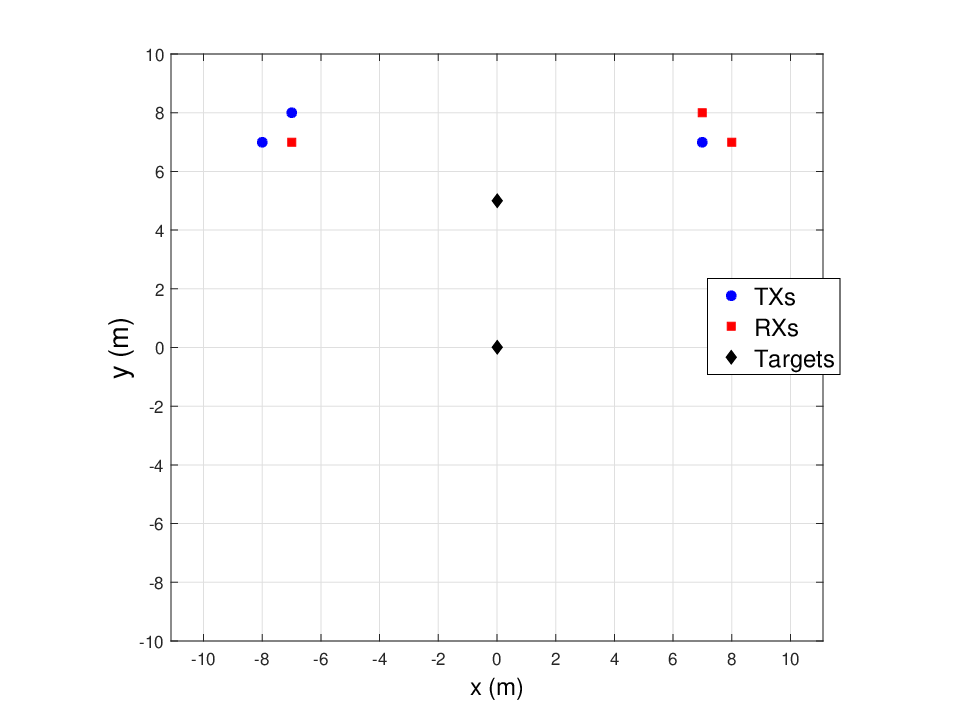
The two algorithms were evaluated over 100 realizations for three values of and and . For each value of , the threshold for the Bayesian MTL algorithm was chosen according to (46). The region of convergence (ROC) curves, plotting versus , for both algorithms are shown in Fig. 3. As expected, they yield identical missed-detection and false alarm rates.
Increasing loosens the compactness constraint on the ellipse intersections around a potential target location, while increasing relaxes the constraint on the probability of a blocking vector/matching. Hence, both and are non-decreasing in and , as seen in Fig. 3. In the special case where only three ellipse intersections are sufficient to declare the presence of a target , the false alarm rates are very high. This is in agreement with the results reported in [34].

V-B Effect of Correlated Blocking
To highlight the effect of correlated blocking, the value of was increased to and the scatterer centers were distributed according to a homogeneous Poisson point process (PPP) of intensity , which amounts to three scatterers in , on average, per realization. The blocking distribution for the PPP scatterer model is derived in Appendix A. A total of 100 network realizations were considered, with and , which corresponds to MPCs per TRP, on average. Let denote the region occupied by scatterers in a given realization. The TX, RX and target locations were uniformly and independently distributed over the region , where ‘’ denotes the set difference operator. Under the i.c.b assumption for the above settings, , where is the average distance between a target and a node. Hence, from (45), for . The distribution of the average number of DPs at a point is tabulated in Table II for both the true blocking distribution and the i.c.b assumption. As per the true blocking distribution, a target has LoS to all TXs and RXs (i.e., 9 DPs) over of the time and the probability that a target has only 3 DPs is a little over . As a result, a matching of size 3 is more likely to be a false alarm. However, since , a matching of size 3 is more probable than a matching of size 9 (which occurs with less than probability) under the i.c.b assumption. As a result, false alarms are identified first, followed by detections, as the value of increases. This is reflected in the ROC curves plotted in Fig. 4, where the i.c.b assumption gives rise to very high false alarm rates.
| Blocking Distribution | 3 | 4 | 5 | 6 | 7 | 8 | 9 | |
|---|---|---|---|---|---|---|---|---|
| True | 0.0700 | 0.0150 | 0.0750 | 0 | 0.1750 | 0 | 0 | 0.6650 |
| i.c.b assumption | 0.3367 | 0.1961 | 0.2578 | 0.2259 | 0.1320 | 0.0496 | 0.0109 | 0.0011 |

V-C Comparison with genie-aided method
In many radar applications, a missed-detection is more costly than a false alarm. As a benchmark, the missed-detection probability of the Bayesian MTL algorithm is compared with that of a genie-aided method, which involves running the Bayesian MTL Algorithm on the true target matchings, in Fig. 5. It can be seen that the proposed algorithm performs as well as the genie-aided method.

V-D Experimental Results
We now present some experimental results that further validate the performance of the Bayesian MTL algorithm. We chose a portion of UltraLab at USC, a cluttered indoor environment, for our measurements. The floor was paved with square tiles of side which provided a natural Cartesian coordinate system, as shown in Fig. 6(a). The measurement setup is shown in Fig. 6(b). For the -th TRP, the frequency response of the ultrawideband (UWB) channel over 6-8 GHz was measured twice at 1601 frequency points - once without the targets (i.e., the background measurement, denoted by ) and then with the targets present (denoted by ) - using a pair of horn antennas with beamwidth , connected to a vector network analyzer (VNA). This corresponds to . Horn antennas were preferred over omnidirectional antennas to restrict the background clutter to a narrow sector. The antennas were maintained at the same height from the ground in order to create a 2D localization scenario, and were oriented to face the targets. Two identical, foil-wrapped cylindrical poles were chosen as the targets. Although the height of the cylinders exceeded that of the TX and RX antennas, the portion of the cylinder that was in the plane of the antennas was wrapped in foil to maintain the 2D nature of the problem.
Let denote the channel impulse response for the -th TRP due to the targets alone (i.e., after background subtraction). Then, is given by the following expression,
| (47) |
The noise floor corresponding to the -th TRP was determined by computing the average power in the last 100 samples of . These delay bins correspond to a signal run length in excess of , which is well in excess of the ranges encountered in our measurement scenario (less than ). Hence, it is reasonable to assume that the energy in these delay bins is due to thermal noise alone. After determining the noise power, MPCs were extracted from whenever the SNR was greater than . A distributed virtual MIMO radar was implemented by moving the TX and RX antennas to different locations, as shown in Fig. 7. Six TRPs were considered, which are indexed in Table III. LoS was present between all TXs, RXs and targets (i.e., ).


| TRP | 1 | 2 | 3 | 4 | 5 | 6 |
|---|---|---|---|---|---|---|
| TX | 1 | 2 | 3 | 3 | 5 | 4 |
| RX | 1 | 2 | 2 | 3 | 3 | 3 |
The estimated target locations are plotted in Fig. 8, from which the following inferences can be drawn:

- (i)
Setting ensures that only those points at which all six ellipses (corresponding to the six TRPs) intersect are detected as target locations. It can be seen that both targets are localized.
- (ii)
The Bayesian MTL algorithm was formulated under the assumption of point targets. Since the targets are not point objects, multiple DPs are possible, in general, for each target. As a result, we obtain a cluster of location estimates for each target location.
- (iii)
The DPs to the targets are at least 10 dB above the noise floor post background cancellation, even in a cluttered environment, which can be attributed to the targets being strong reflectors and having a sufficiently large radar cross-section, due to the foil wrapping.
- (iv)
The steel pillar to the left of Target 1, which is a part of the clutter, was still ‘localized’ in spite of background subtraction. In terms of range, Target 1 and the pillar are closely separated for all the TRPs. Hence, some of the energy from the DP to Target 1 spills over into the delay bin corresponding to the pillar location. As a result, the pillar cannot be perfectly canceled out during background subtraction. The residual energy manifests itself as a DP to the pillar, leading to its localization. An implication of this is that the background in the immediate vicinity of a target cannot be subtracted completely.
VI Summary and Conclusions
In this paper, we considered the impact of environment-induced correlated blocking on localization performance. We first provided a theoretical framework for MTL using a distributed MIMO radar by formulating the general problem of localizing all the targets and scatterers in an unknown environment as a Bayesian estimation problem. We then proceeded to derive a more tractable approximation, known as the Bayesian MTL problem, where the objective was to localize only the targets, but not the scatterers. We then proposed a polynomial-time approximation algorithm - at the heart of which was a blocking-aware vector likelihood function that took correlated blocking into account - to solve this problem. The algorithm relies on two thresholds, and , to detect targets and works with either theoretical or empirical blocking statistics that may be obtained via measurements or simulations. Our simulations showed that ignoring correlated blocking can be lead to very poor detection performance, with false alarms being more likely to occur than detections, and our experiments yielded encouraging results, even in the presence of non-idealities such as improper background subtraction and non-point targets.
VII Acknowledgments
The authors would like to thank C. Umit Bas, O. Sangodoyin and R. Wang for their assistance in carrying out the measurements.
Appendix A Blocking model
Let the scatterers be represented by balls of diameter , whose centers are distributed according to a homogeneous PPP with intensity . For LoS to exist between two points separated by a distance , no scatterer center should lie within a rectangle of sides and (Fig. 9). Therefore, the LoS probability is .

Consider a consistent blocking vector at . The set of nodes that are blocked/unblocked at is determined by and . For each unblocked node, there exists a rectangle which cannot contain any scatterer center. The LoS polygon, , is the union of such rectangles (shaded grey in Fig. 10). In contrast, for each blocked node , there exists an NLoS polygon - the portion of its rectangle not contained in - which must contain at least one scatterer center. Let denote the number of blocked nodes. Then,
| (48) |
where denotes the area operator, acting on sets in . The expression in (48) is a lower bound since it ignores overlapping NLoS polygons which may share scatterer centers (e.g., TX 2 and TX 3 in Fig. 10). The bound is met with equality when none of the NLoS polygons overlap.

References
- [1] S. Steineger, M. Neun, A. Edwardes, and B. Lenz, “Foundations of location based services,” 2006. [Online]. Available: http://www.e-cartouche.ch/content_reg/cartouche/LBSbasics/en/text/LBSbasics.pdf
- [2] “SELECT: Smart and efficient location, identification and cooperation techniques.” [Online]. Available: http://www.selectwireless.eu/home.asp
- [3] K. Witrisal et al., “High-accuracy localization for assisted living: 5G systems will turn multipath channels from foe to friend,” IEEE Signal Processing Magazine, vol. 33, no. 2, pp. 59–70, March 2016.
- [4] E. Karapistoli, F. N. Pavlidou, I. Gragopoulos, and I. Tsetsinas, “An overview of the IEEE 802.15.4a standard,” IEEE Commun. Mag., vol. 48, no. 1, pp. 47–53, January 2010.
- [5] A. Haimovich, R. Blum, and L. Cimini, “MIMO radar with widely separated antennas,” IEEE Signal Process. Mag., vol. 25, no. 1, pp. 116–129, 2008.
- [6] Y. Bar-Shalom and X. Li, Multitarget-multisensor Tracking: Principles and Techniques. Storrs, CT, USA: Yaakov Bar-Shalom, 1995.
- [7] R. Mahler, Statistical Multisource-Multitarget Information Fusion. Norwood, MA, USA: Artech House, 2007.
- [8] J. Shen and A. F. Molisch, “Estimating multiple target locations in multi-path environments,” IEEE Trans. Wireless Commun., vol. 13, no. 8, pp. 4547–4559, Aug 2014.
- [9] H. Godrich, A. Haimovich, and R. Blum, “Cramer-Rao bound on target localization estimation in MIMO radar systems,” in Information Sciences and Systems, 2008. CISS 2008. 42nd Annual Conference on, March 2008, pp. 134–139.
- [10] Z. Zheng, J. Zhang, and Y. Wu, “Multi-target localization for bistatic MIMO radar in the presence of unknown mutual coupling,” Systems Engineering and Electronics, Journal of, vol. 23, no. 5, pp. 708–714, Oct 2012.
- [11] J. Li, H. Li, L. Long, G. Liao, and H. Griffiths, “Multiple target three-dimensional coordinate estimation for bistatic MIMO radar with uniform linear receive array,” EURASIP Journal on Advances in Signal Processing, vol. 2013, no. 1, pp. 1–11, 2013.
- [12] H. Yan, J. Li, and G. Liao, “Multitarget identification and localization using bistatic MIMO radar systems,” EURASIP J. Adv. Signal Process, vol. 2008, pp. 48:1–48:8, Jan. 2008. [Online]. Available: http://dx.doi.org/10.1155/2008/283483
- [13] F. Liu and J. Wang, “An effective virtual ESPRIT algorithm for multi-target localization in bistatic MIMO radar system,” in Computer Design and Applications (ICCDA), 2010 International Conference on, vol. 4, June 2010, pp. V4–412–V4–415.
- [14] A. Gorji, R. Tharmarasa, and T. Kirubarajan, “Tracking multiple unresolved targets using MIMO radars,” in 2010 IEEE Aerospace Conference, march 2010, pp. 1 –14.
- [15] C. Duofang, C. Baixiao, and Q. Guodong, “Angle estimation using ESPRIT in MIMO radar,” Electronics Letters, vol. 44, no. 12, pp. 770–771, 2008.
- [16] C. Jinli, G. Hong, and S. Weimin, “Angle estimation using ESPRIT without pairing in MIMO radar,” Electronics Letters, vol. 44, no. 24, pp. 1422–1423, Nov. 2008.
- [17] M. Jin, G. Liao, and J. Li, “Joint DoD and DoA estimation for bistatic MIMO radar,” Signal Processing, vol. 89, no. 2, pp. 244–251, 2009.
- [18] J. L. Chen, H. Gu, and W. M. Su, “A new method for joint DoD and DoA estimation in bistatic MIMO radar,” Signal Processing, vol. 90, no. 2, pp. 714–718, 2010.
- [19] H. L. Miao, M. Juntti, and K. Yu, “2-D unitary-ESPRIT based joint AoA and AoD estimation for MIMO systems,” in IEEE PIMRC, 2006.
- [20] A. A. Gorji, R. Tharmarasa, W. Blair, and T. Kirubarajan, “Multiple unresolved target localization and tracking using colocated MIMO radars,” IEEE Transactions on Aerospace and Electronic Systems, vol. 48, no. 3, pp. 2498–2517, 2012.
- [21] W. Xia, Z. He, and Y. Liao, “Subspace-based method for multiple-target localization using MIMO radars,” in IEEE International Symposium on Signal Processing and Information Technology, 2007, pp. 715–720.
- [22] L. Xu and J. Li, “Iterative generalized-likelihood ratio test for MIMO radar,” IEEE Transactions on Signal Processing, vol. 55, no. 6, pp. 2375–2385, 2007.
- [23] Q. He, R. Blum, and A. Haimovich, “Noncoherent MIMO radar for location and velocity estimation: More antennas means better performance,” Signal Processing, IEEE Transactions on, vol. 58, no. 7, pp. 3661–3680, July 2010.
- [24] R. Niu, R. Blum, P. Varshney, and A. Drozd, “Target localization and tracking in noncoherent multiple-input multiple-output radar systems,” Aerospace and Electronic Systems, IEEE Transactions on, vol. 48, no. 2, pp. 1466–1489, APRIL 2012.
- [25] Y. Ai, W. Yi, G. Cui, and L. Kong, “Multi-target localization for noncoherent MIMO radar with widely separated antennas,” in Radar Conference, 2014 IEEE, May 2014, pp. 1267–1272.
- [26] C. K. Kim and J. Y. Lee, “ToA-based multi-target localization and respiration detection using UWB radars,” EURASIP Journal on Wireless Communications and Networking, vol. 2014, no. 1, 2014.
- [27] J. A. Hogbom, “Aperture synthesis with a non-regular distribution of interferometer baselines,” Astronomy and Astrophysics Supplement, vol. 15, pp. 417–426, June 1974.
- [28] A. Richter, “Estimation of Radio Channel Parameters: Models and Algorithms,” Ph. D. dissertation, Technischen Universität Ilmenau, Germany, May 2005, ISBN 3-938843-02-0.
- [29] J. Salmi and A. F. Molisch, “Propagation Parameter Estimation, Modeling and Measurements for Ultrawideband MIMO Radar,” IEEE Transactions on Antennas and Propagation, vol. 59, no. 11, pp. 4257–4267, nov. 2011.
- [30] X. Chen, H. Leung, and M. Tian, “Multitarget detection and tracking for through-the-wall radars,” IEEE Transactions on Aerospace and Electronic Systems, vol. 50, no. 2, pp. 1403–1415, April 2014.
- [31] R. Zetik, M. Eschrich, S. Jovanoska, and R. S. Thoma, “Looking behind a corner using multipath-exploiting UWB radar,” IEEE Transactions on Aerospace and Electronic Systems, vol. 51, no. 3, pp. 1403–1415, July 2015.
- [32] J. Shen, A. F. Molisch, and J. Salmi, “Accurate Passive Location Estimation Using TOA Measurements,” IEEE Transactions on Wireless Communications, vol. 11, no. 6, pp. 2182–2192, June 2012.
- [33] P. Setlur, G. Smith, F. Ahmad, and M. Amin, “Target Localization with a single sensor via Multipath Exploitation,” IEEE Trans. Aerosp. Electron. Syst., vol. 48, no. 3, pp. 1996–2014, 2012.
- [34] S. Aditya, A. F. Molisch, and H. Behairy, “Bayesian multi-target localization using blocking statistics in multipath environments,” in the IEEE ICC 2015 Workshop on Advances in Network Localization and Navigation (ANLN), June 2015.