Orbital tori for non-axisymmetric galaxies
Abstract
Our Galaxy’s bar makes the Galaxy’s potential distinctly non-axisymmetric. All orbits are affected by non-axisymmetry, and significant numbers are qualitatively changed by being trapped at a resonance with the bar. Orbital tori are used to compute these effects. Thick-disc orbits are no less likely to be trapped by corotation or a Lindblad resonance than thin-disc orbits. Perturbation theory is used to create non-axisymmetric orbital tori from standard axisymmetric tori, and both trapped and untrapped orbits are recovered to surprising accuracy. Code is added to the TorusModeller library that makes it as easy to manipulate non-axisymmetric tori as axisymmetric ones. The augmented TorusModeller is used to compute the velocity structure of the solar neighbourhood for bars of different pattern speeds and a simple action-based distribution function. The technique developed here can be applied to any non-axisymmetric potential that is stationary in a rotating from – hence also to classical spiral structure.
Keywords:
Galaxy: kinematics and dynamics – galaxies: kinematics and dynamics – methods: numerical1 Introduction
From numerically integrated orbits in model gravitational potentials it has long been known that most orbits in a galaxy are quasiperiodic (Binney & Spergel, 1982; Binney & Spergel, 1984). One may show that any quasiperiodic orbit is confined to a three-dimensional torus in six-dimensional phase space (Arnold, 1989). It is convenient to label each such torus by the Poincaré invariants associated with three closed paths around the torus that cannot be deformed into one another without leaving the torus (Binney & Tremaine, 2008, e.g.). These labels are known as actions , and they are singled out from other integrals of motion, in particular energy, in that can be complemented by canonically conjugate “angle” variables . The latter quantify position within a torus.
Usually orbital tori are nested one inside another, so a non-negligible volume of phase space is filled by such a set of nested tori, and the coordinates constitute an exceedingly convenient set of canonical coordinates for this region. In certain exceptional potentials a single system of tori completely fills phase space, so there is a global system of action-angle coordinates. Such potentials are said to be “integrable”. The potentials studied by Stäckel and named after him (Binney & Tremaine, 2008, e.g.), which yield separable Hamilton-Jacobi equations, are the best known and most important integrable potentials.
By Jeans’ Theorem (Jeans, 1915) the distribution function (DF) of a steady-state galaxy can be assumed to be a function of whatever isolating integrals are admitted by the galaxy’s potential. Hence wherever in phase space orbits are quasiperiodic, we may take the DF to be a function of the action integrals, and there are cogent reasons (Binney & McMillan, 2016, e.g.) why it is advantageous to assume that depends only on rather than directly on the Hamiltonian , as has normally been assumed in the past. If the galactic potential is integrable, the DF can be a single function of , while if phase space breaks up into two or more regions, each with its own sequence of nested tori, each region will require its own functional form, and the global DF will be made up of a patchwork of functions , each with its own domain of validity.
In a fairly realistic Galactic potential, the orbits of some halo stars near the Sun lie on tori that do not belong to the family that in an integrable potential fills all phase space (Binney & McMillan, 2016; Binney, 2016, hereafter B16). B16 showed that a remarkably precise quantitative understanding of the orbits of these stars can be achieved through the concept of resonant trapping. Specifically, one uses the torus-mapping technique (Binney & McMillan, 2016) to construct an integrable Hamiltonian that rather closely approximates the true Hamiltonian, and then one uses first-order perturbation theory to compute the libration of orbits around resonant orbits in the integrable Hamiltonian.
The trapping discussed by B16 involved the 1:1 resonance between the radial and vertical oscillations of stars. An observational signature of such resonant trapping has yet to be detected, but since the work of Dehnen (1998), who used Hipparcos data to map velocity space for stars near the Sun, it has been known that there are features in this space that are inconsistent with the hypothesis that the DF has the form with the actions of an integrable axisymmetric potential.
It has long been suspected that non-axisymmetric components of the Galactic potential are responsible for the differences between observations and the predictions of models that assume axisymmetry (De Simone et al., 2004; Sellwood, 2010; Hahn et al., 2011; Antoja et al., 2011; McMillan, 2013; Pérez-Villegas et al., 2017). Indeed, the Galaxy is known to have a bar, that may extend as far out as (Blitz & Spergel, 1991; Binney et al., 1991; Sormani et al., 2015; Wegg et al., 2015), and the disc is known to carry spiral structure (Lépine et al., 2011, e.g.). Consequently, the assumption of axisymmetry, which has been used with considerable success in a large number of papers (Binney, 2012b; Bovy & Rix, 2013; Piffl et al., 2014; Binney & Piffl, 2015) cannot be more than a starting point for a more sophisticated treatment that includes the bar and spiral structure.
The goal of this paper is to lay the foundations for such modelling by adapting the perturbative approach of B16 to non-axisymmetric potentials. Specifically, a simple model of the Galactic bar is used to trap the tori of a realistic Galactic potential around the corotation and outer Lindblad resonances (CR, OLR). Perturbation theory yields an analytic model of the trapped tori, so we have for these trapped tori all the functionality of tori constructed for an axisymmetric potential by torus mapping (Binney & McMillan, 2016).
The paper is organised as follows. In Section 2 we introduce the model of the potential of a barred Galaxy that we employ subsequently. In Section 3 we explain how the Hamiltonian for motion in a steadily rotating barred potential is decomposed into a part that depends only on the actions and a perturbation . In Section 4 we present the relevant Hamiltonian perturbation theory. In Section 5 we apply this theory to our model Galaxy, starting in Section 5.1 with the OLR, proceeding in Section 5.2 to the corotation resonance, and concluding with a very brief description of the ILR in Section 5.3. In Section 6 we use these results to examine velocity space at a solar-like location within our model Galaxy. In Section 7 we relate our results to previous work and consider how our results help us to understand the dynamics of a non-axisymmetric disc. In Section 8 we sum up and consider directions for future work.
Appendix A describes enhancements to the publically available code Torus Mapper (tm), which enable one to construct and manipulate non-axisymmetric orbital tori, whether resonantly trapped or circulating. TM can be can be downloaded from https://github.com/PaulMcMillan-Astro/Torus. Appendix B provides the theoretical structure that tm uses to find the velocities at which a trapped torus passes through a give point.
We use throughout Galactocentric polar coordinates with the long axis of the bar along . Quantities referring to the azimuthal angle are always listed last because in an axisymmetric potential motion in is slaved by angular-momentum conservation to the autonomous and sometimes complex motion in the -plane.
2 The Galactic potential
We frame our discussion in the context of a gravitational potential that McMillan (2011) fitted to a variety of data for our Galaxy. Specifically, we adopt the “best” potential in that paper, which is generated by thin and thick stellar discs, a flattened (axisymmetric) bulge and a spherically symmetric dark halo. Its local circular speed is . Our discussion would not differ materially, however, had we adopted any reasonably realistic axisymmetric potential. To evaluate the potential and its derivatives we use the falPot code distributed in the tm package, which implements an algorithm described by Dehnen & Binney (1998), and was extracted from Walter Dehnen’s falcON package (https://github.com/Milkyway-at-home/nemo/tree/master/nemo_cvs/usr/dehnen/falcON).
2.1 Non-axisymmetric component
We add to the axisymmetric potential a non-axisymmetric perturbation, so
| (1) |
The non-axisymmetric contribution to the density is
| (2) |
This should vanish at both small and large radii. In fact, as the axis is approached it must vanish at least as fast as . At large it should tend to the external potential of a quadrupole, so decay like . These conditions are satisfied by the ansatz
| (3) |
where is a scale radius,
| (4) |
and the constant controls the flatness of the non-axisymmetric contribution to the density. The normalising constant in equation (3) has dimensions of velocity squared times length cubed, so it is convenient to control its value through the dimensionless number
| (5) |
where is the circular speed at the solar radius that is implied by the axisymmetric component of the potential.


We now have
| (6) |
so
| (7) |
Similarly
| (8) |
and
| (9) |
From these formulae the density is readily computed.
2.2 Normalisation of the bar
Sormani et al. (2015) simulated the flow in two dimensions of isothermal gas flow in model Galactic potentials and by comparing the simulations to radio-frequency observations of Galactic gas estimated the pattern speed and amplitude of the bar. They concluded that the bar has to generate a substantial quadrupole moment. We fix the strength of our bar by reference to that of their most successful models.
Whereas we have chosen to work from a simple analytic function for the coefficient of proportionality, , Sormani et al. (2015) assumed a particular form for the corresponding density:
| (10) |
where , and is a dimensionless amplitude.
The strength of a bar is quantified by . Since , in the notation of equation (2.95) in Binney & Tremaine (2008) at large
| (11) |
Consequently, at large the potential generated by (10) is
| (12) |
For the integral tends to , so
| (13) | |||||
When so , our expression (3) for yields , so to achieve the same quadrupole as Sormani et al. (2015) we must set
| (14) |
In this formula, we adopt and .
It remains to choose the bar’s scale length, . Guided by plots like those of Figs. 1 and 2, we adopt , which is times the density weighted disc scale lengths of the axisymmetric component. Then the figures show that the surface density is strongly barred inside and significantly non-axisymmetric out to . Vertically the bar extends to .
2.3 Pattern speed
Sormani et al. (2015) concluded that the bar’s pattern speed is , a value that coincides nicely the estimate obtained by Wegg et al. (2015) by modelling the kinematics of bulge stars. Pérez-Villegas et al. (2017) show that correctly predicts the kinematics of solar-neighbourhood stars because it causes stars trapped by corotation to visit the solar neighbourhood in the form of the “Hercules stream”. Over the previous two decades larger values were favoured, in part on account of a significant under-estimate of the length of the bar by Binney et al. (1991) and in part through the Hercules stream being supposed to arise by trapping at the OLR rather than corotation (Dehnen, 1998; Monari et al., 2017). In the following we adopt .
We take the pattern speed to be positive, so the bar rotates anticlockwise in the plane. We usually consider that our Galaxy rotates clockwise because we imagine viewing it from the Northern hemisphere. To apply the present model to our Galaxy we must view the latter from Australia. The end of the bar that is nearer to the Sun is rotating away from the Sun. We achieve a similar location for a model Sun by placing it at degrees.
3 Splitting the Hamiltonian
Our goal is to handle perturbations to an axisymmetric system that rotates at a constant angular velocity . Let be the velocity of a star in the frame of reference that rotates with the system, then the star’s kinetic energy is
| (15) |
so the Lagrangian is
| (16) |
where the original time dependence of the gravitational potential has been absorbed into the rotation of the reference frame. It follows from equation (16) that the canonical momentum is
| (17) |
which is in fact the momentum in the underlying inertial frame. The Hamiltonian is
| (18) |
Since is the inertial-frame momentum, the first two terms on the right of equation (18) comprise the star’s energy in the inertial frame, and the final term is simply , where is the component of angular momentum parallel to . Hence we can write
| (19) |
where is the Hamiltonian that would apply if the given potential were not rotating but stationary in an inertial frame. The shift from to that encodes rotation of the potential changes only one equation of motion, namely that of :
| (20) |
In the rotating frame, increments more slowly than in the inertial frame because the zero-point of angle is advancing at the rate .
By torus mapping it will usually be possible to construct a Hamiltonian that admits a global system of angle action coordinates and is very close to . That is, we can write
| (21) |
where . If is not very strongly non-axisymmetric, we can map tori in such a way that is axisymmetric, so is one of the actions in the set . In this case, the true Hamiltonian
| (22) |
has been successfully split into a dominant part
| (23) |
that does not depend on the angle variables and a small perturbation .
It will sometimes be expedient to map tori in such a way that is non-axisymmetric. If we do map tori thus, we should be able to arrange for to provide a closer approximation to , and thus make smaller than if we keep axisymmetric. The disadvantage of making non-axisymmetric is that then will not coincide with any of the actions in the set – the way each action depends on depends on the potential , and when is non-axisymmetric will not be an action variable. However, as the degree of non-axisymmetry vanishes, one of the actions, which we may call , will converge on . With a non-axisymmetric , the term in the full Hamiltonian will contribute to the perturbative part of the Hamiltonian alongside . That is, in this case we must write
| (24) |
such that the entire square bracket is a perturbation on the integrable Hamiltonian that is defined by the curly bracket. The residual from tm will be substantially smaller than the full non-axisymmetric component of the potential with which we will contend, but this gain will be to some extent offset by the appearance of the perturbation . We leave exploration of this approach to a later study.
4 Resonance
Now we present the theory of resonant trapping. This theory relates to the state of being trapped by a resonance and does not address the complex process by which a star becomes trapped, for example as a bar strengthens and slows down, with the consequence that it sweeps into its embrace stars that previously orbited freely outside it. There is significant overlap between this section and Section 5 of B16, but there are some subtle differences and we need to establish notation for subsequent use.
4.1 Pendulum dynamics
A resonant orbit in is one on which
| (25) |
where is a vector with integer components and
| (26) |
is the vector of frequencies. In the rotating frame, changes sign at corotation from positive inside corotation to negative outside it. Hence to satisfy equation (25) with , the ratio has to rise from negative values inside corotation, through zero at corotation to positive values outside corotation. The best known resonances of this class are the inner Lindblad resonance, , the ultraharmonic resonance , the corotation resonance and the outer Lindblad resonance, . B16 examined the case and we can exploit the formalism developed there by simply replacing in the formulae of B16 by .
Near a resonance, the angle variable
| (27) |
evolves slowly and we make a canonical transformation to new angle-action variables that include this variable. We use the generating function
| (28) |
which ensures that equation (27) holds and makes . From we find
| (29) | ||||||
| (30) | ||||||
| (31) |
We Fourier expand the Hamiltonian in the new angle variables
| (32) |
where . The new actions have the equations of motion
| (33) |
Averaging these equations over the fast angles we conclude that the actions are effectively constant under the perturbation, so we need consider only the system’s motion in the plane. This motion is governed by the Hamiltonian
| (34) |
where and we have omitted references to the constant actions . Since this a time-independent Hamiltonian, the motion occurs on the curve in the plane on which , a constant. A good approximation to this motion can be obtained by Taylor expanding the functions of in equation (34). However, before we do so we exploit the reality of to write
| (35) |
where the are the amplitudes and are the phases of the complex variables . We expand and to second order in
| (36) |
where is the primed action of the resonant torus. Since a constant term in can be discarded and we know that on the resonant torus (eq. 25), we replace by , where
| (37) |
The Taylor series for ,
| (38) |
cannot be simplified in this way, so the equation becomes
| (39) | ||||
| (40) | ||||
| (41) |
In this approximation we can determine simply by solving the quadratic equation (39) for given . Given the oscillating value of and the constants , we can recover the complete action-space coordinates from equations (29). In general all three components of oscillate but in such a way that is to leading order constant.
If we retain only one value of and neglect and , equation (39) reduces to the energy equation of a pendulum, and this is traditionally used to discuss resonant trapping (Chirikov, 1979, e.g.). Kaasalainen (1994) demonstrated the merit of retaining and . B16 retained two values of , but we shall find in the applications considered here that there is only one value of to consider.
4.2 Action and angle of libration
The range through which oscillates is set by the condition that the quadratic for has real roots:
| (42) | ||||
| (43) |
When , as is the case at both OLR and CR, condition (42) is satisfied for the widest range of angles when also, so the second bracket on the right is often positive. If is less than a critical value , the condition is satisfied but for no value of becomes by equality. Consequently, at no value of do the roots coincide, and the orbit is restricted to one root or the other. This is the regime of circulation. The two roots corresponds to circulation inside and outside the region of entrapment.
When is larger than , condition (42) is satisfied in a restricted range in , and an orbit can transfer from one root to the other at the extremes of this range. This is the regime of libration. As increases, the range shrinks and it vanishes at . When the amplitude of libration vanishes.
In the case of the OLR we find that and vanishes for and that . So when and are neglected, the libration condition is
| (44) |
Given that the are by definition all non-negative, it follows that libration occurs around . Hence, when , equation (44) forces , and the libration amplitude vanishes. Conversely, when the libration amplitude becomes . It follows that is the value of for which condition (42) is an equality with the cosines set to , while is the value of at which equality is reached with the cosines equal to .
Each value of in the range corresponds to an action that quantifies the extent to which a trapped orbit oscillates around the trapping torus. is straightforwardly computed as
| (45) |
where the dependence of on is obtained from equation (39). Since increases from its minimum to its maximum value with given by the larger root of the quadratic (39) and returns to its minimum value with given by the smaller root, is give by the difference of the roots integrated over the range of .
The procedure for computing the actions of circulating orbits is very similar: one averages the relevant root with respect to and then adds this average to the value of for the perfectly resonant torus to obtain the value of on the newly created torus.
On a trapped or nearly trapped orbit, is not an angle variable, although are angle variables. Since the missing angle variable evolves linearly in time, it is
| (46) |
where from Hamilton’s equation and equation (35) we have
| (47) |
In this equation is by the quadratic equation (39) a function of .

4.3 Impact of non-resonant terms
Above we neglected all non-resonant terms by averaging the equations of motion (33) over the fast angles. This procedure works extremely well when the tori are fitted to the full Hamiltonian rather than just a symmetric part of it because the fitting procedure can, in principle, reduce the non-resonant terms in the Fourier decomposition of to arbitrarily small values. Unfortunately, in the present case the torus is fitted to the axisymmetric part of and the variation of H over the fitted tori include significant non-resonant terms. We should include these terms in the perturbative treatment.
Fig. 3 illustrates this point by showing the values of the for a torus on which the condition for the OLR is perfectly satisfied. The largest term is non-resonant, being proportional to . There follow a series of terms that are proportional to . Of these terms only the largest, which has , is resonant. The impact of this term was computed above. Here we compute the impact of the non-resonant terms.
It is convenient to work in the coordinate system in which, according to the theory of Section 4.1, and are constant, while obeys a pendulum equation. The non-resonant terms induce small oscillations in and slightly modify the pendulum motion of .
We consider first the largest non-resonant term, which is a particularly simple case because it has and the only equation of motion affected by this term is that for . Moreover , so we may write
| (48) |
Integrating this equation, it follows that
| (49) |
where denotes the average value of , which we interpret to be value of for the perfectly resonant torus. It is perhaps worth noting that equation (49) could have been obtained by requiring that at any point on the orbit the change in the unperturbed Hamiltonian,
| (50) |
cancel the numerical value of the perturbing Hamiltonian.
In a similar vein, the contributions of the other non-resonant terms to the equations of motion are
| (51) | |||||
When we set and these equations are equivalent to equation (49) for the change induced by the largest perturbation.
4.4 Resonant or non-resonant theory?
The point of the pendulum equation is that it yields an accurate representation of the non-uniform evolution of the resonant angle . The equation’s weakness is that it derives its data from the immediate vicinity of the perfectly resonant torus. Specifically, we use with it values of and the resonant Fourier amplitudes that were obtained from Taylor series, but the employed values of the non-resonant amplitudes are simply those of the perfectly resonant torus. Near that torus, the pendulum equation provides accurate results, but as we move away, errors arising from stale values of grow. Meanwhile, as we move deeper into the region of circulation, the motion of the resonant angle becomes faster and more uniform. At some point it becomes advantageous to abandon the pendulum equation and simply apply equations (51), but now including all the rather than just the non-resonant terms, and using the values of and for the current torus rather than for the perfectly resonant torus.
5 Examples
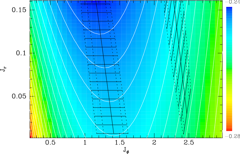
In this section we show results obtained when the formalism of the last section is applied to the Hamiltonian associated with the model Galactic potential of Section 3. In Fig. 4 the colour scale and white contours show the value of the axisymmetric Hamiltonian through a significant part of action space. At a given (small) value of , peaks at the value of associated with corotation. This ridge-line in corresponds to the fact that in a rotating frame the effective potential has the structure of a volcano in that it falls away from a roughly circular rim in the vicinity of corotation into the crater on one side and down towards the flatlands on the other (e.g. Binney & Tremaine, 2008, Figure 3.14). Fig. 4 is computed for vertical action , which typically lets solar-neighbourhood orbits reach . However, the diagram computed for , which lets stars reach , is virtually indistinguishable. Thus the response of stars to the bar will not depend on whether they belong to the thin or thick disc.
Two black ladder-like structures are evident in Fig. 4. The left-hand ladder marks the region within which stars are trapped at corotation, while the right-hand ladder marks the region of entrapment by the OLR. The line down the centre of each ladder marks the tori on which the relevant resonance condition is exactly satisfied. The shorter lines or “rungs” that cross this central line are the tangents to the contours of constant where they cross the central line. During libration the locations of orbits in the plane oscillate parallel to these rungs. Each side of the ladder is marked by two parallel lines. The distance across a ladder between the inner lines measures the maximum amplitude of libration of trapped orbits, which is simply the value of the libration action obtained by setting in the pendulum formulae. The outer lines indicate the furthest excursions of trapped orbits from the actions of the underlying perfectly resonant orbit. Within the phase space associated with the gap between the inner and outer lines there are orbits that librate and orbits that circulate. These orbits are all best computed with resonant perturbation theory, while outside this region non-resonant theory is usually more reliable.


5.1 Trapping at the OLR
Fig. 5 shows a typical orbit trapped at the OLR. The red curve shows the trajectory yielded by perturbation theory, while the black curve shows the trajectory obtained by numerically integrating the full equations of motion from a single phase-space point on the red trajectory. Since perturbation theory yields a close approximation to an orbit, starting the black trajectory from a different point makes very little difference to the figure.
Fig. 6 is a surface of section at and . The full curves are cross sections through tori in the axisymmetric Hamiltonian obtained by torus mapping (Binney & McMillan, 2016). The condition for resonance at the OLR is satisfied on the middle torus, and the tori generating the outermost and innermost curves are the tori that perturbation theory predicts will bound the region of entrapment.
The points in Fig. 6 are consequents of seven orbits integrated with the full equations of motion from initial conditions on the resonant torus. The consequents of any given orbit lie on a curve because these are quasiperiodic orbits. But for only two orbits does this curve resemble the cross section of a torus generated by tm. It is evident that on the orbits that gave rise to the innermost and outermost sets of consequents the resonant angle circulates, while in the intervening five orbits librates. We see that the boundaries of the region of entrapment are quite accurately predicted by perturbation theory. The cross sections of the tori almost coincide at small but this is an illusion: the tori have distinct values of , with the consequence that at a given they are well separated in .
The upper panel of Fig. 7 shows the same surface of section as Fig. 6 but with the cross sections through tori of now shown in broken blue lines. The full black curves in Fig. 7 are cross sections through tori computed with the perturbation theory presented above. The points are consequents obtained by integrating the full equations of motion from one phase-space point on each full curve. The orbit shown in Fig. 5 produces consequents that lie just outside the outermost of the curves of trapped orbits. The agreement between the points and the full curves is excellent, both for the four orbits that librate and for the fifth, circulating orbit, on which .
The lower panel of Fig. 7 is similar to the upper panel but for the case that the perfectly resonant torus has . The orbit with the maximum amplitude of libration around this resonant torus comes close to the torus in the course of its libration, so the innermost blue curve is small.
To obtain the results from perturbation theory plotted in Fig. 7, one has to be able to predict given arbitrary values . Given a value of , the associated torus is constructed by interpolation on a grid of ten tori that lie along the edge of a rectangle five grid points wide and two grid points high in the plane. It proves advantageous for the grid to be uniformly spaced in rather than in as the worst interpolation errors arise near the “skinny” torus that lies on the axis in Fig. 4. The axisymmetric tori that generated the broken blue curves in Fig. 7 lie along the long axis of the rectangle and were obtained by interpolating between pairs of tori that have the same value of . Their near-uniform increase in radius reflects their uniform spacing in .
The area enclosed by each broken curve in Fig. 7 is proportional to the value of on the corresponding torus. Thus in the upper panel all these tori have non-negligible values of , but in the lower panel, associated with a resonant orbit that has less radial action by a factor , the innermost broken blue curve has a very small area and thus corresponds to an essentially circular orbit. The area inside each full black curve is proportional to the value of the resonant action (eqn 45). At the centre of the island of full curves would lie the single consequent generated by the closed trapped orbit , which we can obtain by setting .
5.2 Trapping at corotation
Unfortunately, a slight adjustment to the theory of Section 4 is required before we apply it to the corotation resonance because at corotation the slow angle is , so if equations (29) are to apply we must re-order our unperturbed angles and actions such that
| (52) |
This done, the previous analysis is valid with , with the result that we do not need to distinguish between and . The impact of the non-resonant terms is now as follows. A term changes the actions by
| (53) | |||||


The resonant term in the Hamiltonian has , so trapped orbits librate around , which corresponds to a point on the minor axis of the potential – in the limit this coincides with the Lagrange point L4. Fig. 8 shows a trapped orbit, in black as computed by integration of the full equations of motion and in red as computed from perturbation theory after reflection in the axis to avoid overplotting the numerically integrated version. This orbit has a relatively large amplitude of libration so it reaches all the way to the long axis of the bar. In fact, this orbit supports the bar quite strongly because the star lingers at the turning points of its libration, when it lies near the axis. The loops along the orbit’s inner and outer crescents are clearly arise from radial oscillations that have a much shorter period than the period of libration. The only significant difference between the red and black versions of the orbit is a small change in the ratio of these periods.
Fig. 9 is a surface of section for orbits with the same radial and vertical actions [] as the orbit shown in Fig. 8. The full curves are the predictions of perturbation theory for five values of while the data points were generated by integrating the full equations of motion from a single point on each of the perturbed tori. Each orbit generates two crescents: the orbit with the largest libration amplitude generates the crescents on the extreme left and the extreme right, the orbit with the second largest libration amplitude generates the next two crescents in, and so on. As is to be expected, the agreement between the data points and the full curves deteriorates as the amplitude of libration increases.
Since we have imposed the requirement , all points arise from times at which the star lies inside its guiding-centre radius and thus is moving progradely in the corotating frame. That is, all points arise not too far from pericentre. If the restriction is lifted, each crescent is complemented by an oppositely directed crescent so each orbit contributes two ellipses to the diagram, one centred on smaller radii than the other. The figure is then too busy to be helpful.
The broken blue curves in Fig. 9 show the points generated by three tori of constructed by interpolation along the centre of the grid of tori from tm that underpins the construction of the non-axisymmetric tori. Both the data points and the full curves track these broken curves to a remarkable extent. However, in an axisymmetric potential each orbit would generate only one crescent, that associated with its angular momentum. In the non-axisymmetric potential orbits generate two crescents because they cross the minor axis with one of two values of . The alignment of the full and broken curves signifies that the angular momentum with which a star returns to the minor axis is independent of the phase of its radial oscillations.


5.2.1 Circulating orbits
When tm fits tori to the full Hamiltonian, as in B16, everything one needs to know about an orbit that circulates rather than librates can be obtained directly from tm. Here, however, tm fits tori to only the axisymmetric part of the Hamiltonian, so perturbation theory is required to obtain a good fit to an orbit that circulates – in fact, the orbit can be significantly non-axisymmetric. Fig. 10 illustrates this point by showing orbits that have slightly too much (upper panel) and slightly too little (lower panel) angular momentum to be trapped by the corotation resonance. Both orbits are far from axisymmetric. As in Fig. 8 the black curves show the orbits obtained by direct integration of the equations of motion and the red curves show the orbits obtained with perturbation theory. The main difference between the black and red curves is the spacing between the loops to which radial oscillations give rise: along the black curve in the upper panel the loops are closer together, indicating that lies close to an integer, whereas along the red curve the loops are more clearly separated indicating a value of that lies less close to an integer.

Fig. 11 shows a surface of section. The orbit plotted in the upper panel of Fig. 10 produces the complete circuit of consequents on the right. The curve on which they lie was computed with perturbation theory. To set the context, we show on the left of this surface of section the consequents and invariant curves of two orbits with the same values of and but with , so they librate. For these orbits, as in Fig. 9, we only show consequents associated with , whereas for the circulating orbit we show consequents for both signs of . This is why the invariant curve of the circulating orbit closes on itself, whereas the invariant curves of the other two orbits form pairs of crescents, one for each of the two values of angular momentum at which the star crosses the bar’s minor axis. The broken blue curves show cross sections through five axisymmetric tori located along the central spine of the grid of tori from tm that formed the basis for interpolation. The broken blue curve on the right, associated with the largest angular momentum, keeps quite close to the black invariant curve of the circulating orbit, indicating that as the latter passes the minor axis, its angular momentum lies in a narrow range. This does not imply, however, that the orbit’s angular momentum is nearly constant: near the major axis it has substantially more angular momentum.
The above reconstruction of a circulating orbit was obtained from the pendulum equation. As such it relies on the determination of the Fourier coefficients on the perfectly resonant torus, which is at some distance from it in phase space.
As was noted in Section 4.4, when an orbit is obtained from resonant perturbation theory, one is using Fourier coefficients of that are becoming increasingly stale as one progresses away from the region of entrapment. At some point it becomes expedient to adopt non-resonant perturbation theory, for then the Fourier coefficients employed are computed locally, on the unperturbed tori over which the orbit is actually ranging. The analytic work of Monari et al. (2016) is based on this type of perturbation theory.
The red curve in Fig. 12 shows the orbit that circulates just outside the region of entrapment by corotation as obtained from non-resonant perturbation theory, with the black curve as usual showing the result of direct numerical integration. We see that non-resonant perturbation theory recovers the shape of the orbit well, but comparison with the upper panel of Fig. 10, which shows the same orbit computed with resonant perturbation theory, reveals a failure to recover the way the orbit lingers along the axis. This is a natural consequence of the key approximation of non-resonant theory, namely that the unperturbed angles evolve uniformly in time. Further from the boundary of the region of entrapment, the non-uniform evolution of the unperturbed angle variables becomes less marked and non-resonant perturbation theory comes into its own.
In conclusion, resonant perturbation should be used both inside and close to the region of entrapment, while non-resonant theory should be used elsewhere.
5.3 Trapping at the ILR
To obtain orbits trapped at the inner Lindblad resonance, the code described in Appendix A should be used to construct an instance of resTorus_L with the resonant vector set to . In contrast to the CR and OLR, at the ILR proves positive while vanishes. As a consequence, libration is still around but now the torus with has vanishing libration amplitude while maximum libration amplitude is attained at . Values of smaller than are now forbidden, while values larger than correspond to circulating orbits.
Examples of orbits trapped at the ILR will be given in a forthcoming publication that focuses on resolving difficulties that the current version of tm encounters with orbits that have small and large .
6 Structure of local velocity space
Now we use our non-axisymmetric tori to examine the structure of the velocity distribution of solar-neighbourhood stars. This exercise illustrates both the inconvenience of orbit-based models of galaxies and the relative strength of torus modelling among orbit-based techniques. We define and , so the Sun is at , increases with motion towards the Galactic centre and is the amount by which the star’s motion in the direction of Galactic rotation exceeds that of the Sun. We assume that (Schönrich et al., 2010). For reasons that will become apparent, most results are presented for pattern speed .
6.1 Orbit-based modelling
When one wishes to compute the density or the velocity distribution at a given point in a model, it is enormously desirable to be in possession of an algorithm that computes given , for then the density at position in velocity space is simply and the density can be recovered by integrating over . For an axisymmetric model, or a triaxial model that has zero pattern speed, we can use the Stäckel Fudge (Binney, 2012a; Sanders & Binney, 2015) for this purpose, but the Fudge has yet to be generalised to systems with rotating non-axisymmetric potentials. Algorithms for non-axisymmetric systems that have been used with some success are those of Dehnen (1999) and Monari et al. (2016). Dehnen (1999) evaluated by integrating an orbit from backwards in time while the bar amplitude was reduced to zero, and then evaluated at the computed location in the axisymmetric model. Monari et al. (2016) computed in essentially the same way except they followed orbits backwards analytically using non-resonant perturbation theory in axisymmetric angle-action coordinates. These algorithms rely on the adiabatic invariance of and consequently fail when resonant trapping is important.
Given the lack of robust algorithms for computing from in rotating, non-axisymmetric potentials, nearly all modelling of non-axisymmetric systems (and much modelling of axisymmetric ones too) has been orbit based in the sense that one finds orbits and assigns them weights such that available observational data are consistent with the values predicted by the weighted averages of the orbits. The classic technique is that of Schwarzschild (1979) but important advances have recently made with the “Made-to-Measure” (M2M) technique proposed by Syer & Tremaine (1996) and developed by de Lorenzi et al. (2007), Dehnen (2009), Long & Mao (2010) and Morganti & Gerhard (2012) among others.
The Schwarzschild and M2M techniques differ in (i) how weights are assigned, and (ii) how orbits are used: for each orbit M2M integrates orbits in parallel and for each orbit holds for only a single time, whereas Schwarzschild integrates orbits in series and for each orbit retains at a large number of times. Hence Schwarzschild uses orbits as time series, and computes densities by summing the time intervals during which each star is in a small volume around the point at which the density is required. If orbits are replaced by tori, it becomes easier to compute the density because one then has analytic formulae for and so one can solve for the angles (if any) ` at which the torus visits a given location and evaluate the velocities with which the visits occur. This approach underlies the code for chemodynamical evolution used by Schönrich & McMillan (2016), and also the analysis of data from the LAMOST survey (Deng et al., 2012) presented by Wang et al. (2017). Our non-axisymmetric, sometimes resonantly trapped, tori allow us the extend this technique to the non-axisymmetric problem posed by the solar neighbourhood.

The general plan is to compute tori for a grid in action space and find the velocities (if any) at which each torus visits the Sun. Then the density of the corresponding cells in the plane is incremented by
| (54) |
where is the sampling density that is defined by the grid. The Jacobian, which converts from density in action space to density in velocity space, is provided by tm. Indeed with denoting Cartesian phase-space coordinates and the generating function of the canonical transformation to angle-action coordinates,
| (55) |
so
| (56) |
Taking determinants it follows that
| (57) |
tm does not directly provide the Jacobian on the right because it uses cylindrical polar coordinates. So it provides
| (58) |
6.2 Orbits trapped at corotation
Each point in Fig. 13 shows the velocity with which a torus visits the Sun-like location deg. We plot in red visits by tori that are not resonantly trapped, and in blue or black visits by tori that have been trapped by corotation. If a torus reaches the Sun, it usually does so at four distinct velocities, two with and two with . In Fig. 13 we show only visits with . Then the plot should contain two visits per torus, one on the left and one on the right of a roughly horizontal line. In the region of entrapment at the bottom of the figure, the left-hand visits have been coloured black and the right-hand ones coloured blue. As the action of libration diminishes, the left- and right-hand points converge on the rather bare space where the black and blue points approach one another. This bare region arises because the tori have been sampled uniformly in : the region can be eliminated by sampling more densely at small values of .

The dots in Fig. 13 are arranged in rings because the tori were computed on a grid in action space: for , the grid in is defined by
| (59) |
with , and . Fig. 14 shows the grid points in action space. By making the grid points uniform in we ensure a near uniform distribution of rings in velocity space. Choosing grid points in is challenging because one wants to obtain points near the line . In the lower part of Fig. 13 and in an axisymmetric system, these points would correspond to visits of stars with low that reach the Sun at apocentre, while in the upper portion of the diagram the points correspond to visits at percentre by stars with large . In a non-axisymmetric potential the situation is more complex, but the general idea holds. So for given we compute the values of the generalised angular momentum of visits at apocentre () and at pericentre () and distribute our grid points between these lower and upper bounds on . We need grid points closely spaced near the limiting values because as the Jacobian in equation (54) diverges. Specifically we take
| (60) |
for in integer step. Then the divergence in the Jacobian is cancelled by a matching divergence in the sampling density that reflects divergence of the density of grid points as , which is just about visible in Fig. 14.
Fig. 13 reveals that this strategy has not been entirely successful in that a river of white can be discerned running vertically through most of the red region. In addition, at the very centre of the figure there is a white patch reflecting the finite smallest value adopted: tm has difficulty computing tori for very small actions. This hole could be filled with tori computed with the epicycle approximation, which is at its most precise in this region.
It is worth noting that the difficulty sampling the plane at small is directly related to the fact that the real-space density generated by an orbit always diverges near its boundaries, and by Liouville’s theorem, its velocity-space density has to be low there. Put another way, the velocity-space density along is inevitably contributed by a small number of stars that each contribute a large probability density at .
In Fig. 13 another blemish is evident at about four o’clock: a wedge that is clear of red dots. The bulk of the red points are computed using non-resonant perturbation theory, while the points that bound the region of trapped orbits are computed with resonant perturbation theory – red points are contributed by circulating orbits and black/blue points by librating orbits. Since resonant and non-resonant perturbation theory involve different approximations, their results do not match perfectly across the join (cf Figs 10 and 12). In particular, at the left-hand edge of the red crescent, similar velocities are obtained with different values of , and when this happens, the figure is redder than usual. At the right-hand edge of the crescent, this over-population is compensated by a small empty region. This blemish might be smoothed by shifting the transfer to non-resonant theory further from the region of entrapment.


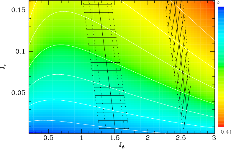
Each point in Fig. 13 is associated with a value of and a value of either (if circulating) or (if librating). Fig. 15 shows the curves (magenta for , broken blue for , black for ) on which these integrals are constant. All points share the same value . In the absence of the bar’s contribution to the potential , we would have so contours of constant would be straight horizontal lines. modifies such that its contours (broken blue) cease to be horizontal and straight. In the region of trapping by CR, (magenta) is complemented by , the action of libration, whose (grey) contours form asymmetric arches.
6.3 Orbits trapped at the OLR
The upper panel of Fig. 15 is for pattern speed , while the lower panel is for . Comparison of these panels reveals how sensitive local velocity space is to the pattern speed. This sensitivity is a consequence of how close the Sun is to the edge at of the region of entrapment by corotation: when is lowered this edge shifts outwards and displacement by a distance that is small compared to is not small compared to .

At the top of Fig. 13, the curves of constant terminate where they encounter the region of entrapment by the OLR. Fig. 16 is the corresponding plot for the faster pattern speed . The regions within which orbits are trapped have both moved down, so the region within which orbits are trapped at OLR is now clearly visible at the top of the figure. The black dots generated by orbits trapped by the OLR line up along curves of constant , which have both left and right branches. Each orbit appears at four points along the curve associated with its value of . Orbits with large values of the libration action appear towards the top and bottom ends of each stubby line of dots, while orbits with small values of appear either side of the middles of these lines. Hence contours of constant delineate a highly elongated and slightly curved island. The OLR region in Fig. 16 contains eleven black and eleven blue lines, and each pair of lines corresponds to the outermost eleven red ellipses, being the ellipses with the largest values of .
Fig. 17 shows the density of stars in the plane that is predicted by a plausible DF . Colours indicate logarithms to base 10 of the density. We base our DF on the work of Piffl et al. (2014), who fitted a DF to data from the Sloan Digital Sky Survey (Jurić et al., 2008, SDSS) and the Radial Velocity Experiment (Steinmetz & et al., 2006, RAVE). Their DF is based on the assumption that the Galaxy is axisymmetric and has to be adapted to encompass non-axisymmetry. The colours and contours in Fig. 18 show the value of the DF in the same slice through action space for which Fig. 4 shows values of . The value of the DF diminishes rapidly with increasing and more gradually with increasing . Since stars trapped at corotation oscillate along the rungs of the figure’s left-hand ladder, they move between regions of high on the left and low on the right. By Jeans’ theorem the value of the true DF must be a function of the constants of motion. Consequently, in the region of trapping we must replace in the argument list of by , the libration action, which controls how far each side of the line of exact resonance a star moves as it librates. In particular, at a given value of , must take the same value just to the right of the dashed line that marks the left-hand boundary of the trapping region as it does just to the left of the dashed line that forms the right-hand boundary of the trapping region. In fact, the simplest possible structure for is that it is constant along each of the rungs of the ladder that marks the trapping region in Figs. 4 and 18. Monari et al. (2017) adopted this ansatz. The actual population will be determined by the precise history of bar formation and lies beyond the scope of this paper. It is, however, a question that can be addressed by an extension of the modelling technique of Aumer et al. (2016).
In the region populated by circulating orbits, we simply evaluate the Piffl et al. (2014) DF on the given numbers . In the region populated by trapped orbits, we evaluate the Piffl et al. DF using the actions of the perfectly resonant orbit from which it obtained by adding some amplitude of libration. This choice leaves the star density in the region of entrapment higher than at points outside this region that are similar distances from the centre of the figure. However, within the trapped zone one can in principle take the DF to be any non-negative function of the integrals .

The observed distribution of local stars in the plane shows an overdensity centred on that is called the Hercules Stream. Dehnen (1999) suggested that it is caused by stars being trapped by the bar’s OLR, and by modelling this process derived . As was noted in Section 2.1, there is now strong evidence that the bar’s pattern speed is not greater than , with the consequence that the OLR lies well outside and could only affect local velocity space at positive values of . With the lower pattern speed we instead lie not far outside the bar’s CR, and Pérez-Villegas et al. (2017) have shown that the model of the bar developed by Wegg et al. (2015) with predicts a feature rather like the Hercules stream that is caused by stars trapped into libration around the Lagrange point L4. Fig. 17 shows that in our model of the bar stars trapped at corotation appear at significantly smaller values of : the region of entrapment does not extend above . On the other hand, it is centred on , rather as in the observations.
The region of entrapment can be moved further up by lowering , or by adopting a locally rising circular-speed curve.
7 Discussion
7.1 Relation to previous work
We have addressed much the same problem as Monari et al. (2016) and Monari et al. (2017) from a rather different perspective. Monari et al. (2016) use angle-action variables to compute the first-order change in an unperturbed DF when a non-axisymmetric component is added to the potential. As a resonance is approached, diverges, so there is a band in action space around a resonant torus within which is not non-negative and hence is manifestly in error. They show that this problem is not mitigated by going to second order. Monari et al. (2017) use the standard pendulum equation to determine the width of the trapping region, but they do not compute actions for trapped orbits, and whenever they use
| (61) |
Using this prescription and the angle-action coordinates provided by the epicycle approximation, Monari et al. (2017) compute the structure of the plane for a variety of pattern speeds and bar strengths. The main differences with our work are (a) we use tori rather than the epicycle approximation so we retain accuracy even for eccentric orbits, (b) we are not restricted to planar orbits, and (c) we have complete control of the DF of trapped orbits, so our DF is finite but discontinuous at the edges of the trapping region as it should be. The practicalities of the two calculations differ significantly because tori provide the transformation while the epicycle approximation provides the inverse transformation . The latter is in many ways the more convenient direction, and by using the Stäckel fudge (Binney, 2012a) for an axisymmetric system one can proceed in this direction without losing accuracy for eccentric orbits. However, the Stäckel fudge is not applicable to rotating non-axisymmetric potentials and it does not tackle resonant trapping, so currently the impact of resonant trapping can only be reliably computed using tori.
Although resonant trapping changes individual orbits qualitatively, Fig. 17 demonstrates that the impact of trapping on velocity space may be quite modest, depending on the form that the DF takes in the region of entrapment. This conclusion probably explains why axisymmetric models such as that of Piffl et al. (2014) have yielded excellent fits to data.
7.2 Poisson noise and modelling strategy
The main difficulty encountered when using tori is getting the sampling density right. For example, in a plot of the plane one wants a dense sampling near the peak of the star distribution, that is near the local standard of rest. Here , etc, are small and small changes in correspond to tiny changes in and . Hence tori must be constructed on a very non-uniform grid in action space. It is similarly necessary to sample densely in near the values for which a star reaches apo- or peri-centre at the location for which the plane is required. Fortunately, torus interpolation makes dense sampling in a particular region computationally affordable, and Fig. 17 demonstrates that the non-uniform action-spaced grid of Fig. 14 provides adequate sampling of circulating orbits. The sampling of resonantly trapped orbits needs refinement, however.
Custom sampling of action space can be avoided by devising an algorithm that interpolates to a general point in velocity space the values taken on a sub-optimal grid by the constants of motion, or as appropriate. An algorithm of this type was used to plot the contours of Fig. 15, and a similar algorithm lies at the heart of the chemodynamical evolution code that underpins Schönrich & McMillan (2016). This procedure seems to be the most promising way forward for chemodynamical modellers.
Poisson noise is a constant irritant when one seeks to model galaxies with precision, so it is a major headache when modelling the Milky way. Indeed, to extract a reasonable plot of the local plane from the M2M model of Wegg et al. (2015), Pérez-Villegas et al. (2017) had to upgrade the model significantly because the solar neighbourhood contains only a very small fraction of the Galaxy’s stars. Plots such as Fig. 17 show that the combination of modelling and torus interpolation enables one to beat Poisson noise down to low levels at small computational cost: even with the current not-optimised version of tm this figure can be computed from scratch in of order half a processor-hour. The plane predicted by a different DF can be computed in less than a second.
In standard Schwarzschild modelling, one starts from a potential and seeks orbit weights that are consistent with and observational constraints. Unless the system is extremely simple, it is not unlikely that cannot be generated by any set of non-negative weights. When tori are employed, one can start with and adjust the weights of tori (or the parameters of DFs for each component) until reasonable agreement with data is achieved. Then one can relax the potential to exact self-consistency (Binney, 2014; Piffl et al., 2015) to obtain a completely sound model. Standard Schwarzschild modelling does not permit this step to self-consistency.
In summary, there are many reasons why classical Schwarzschild modelling, in which orbits are used as time sequences, is abandoned in favour of torus modelling: tori are simply more compact and very much more powerful than classical orbits. In point of historical fact, Martin Schwarzschild himself took the first step towards torus modelling (Ratcliff et al., 1984).
7.3 Accuracy and chaos
The quality of the fits delivered by perturbation theory is remarkable. For example, the length of black ladder rungs in Fig. 4 and the qualitative difference between the full black and broken blue invariant curves in Fig. 7 show that along an orbit trapped by the OLR the angular momentum and radial action typically make large excursions and trapped orbits do not keep close to the perfectly resonant torus which provides the numbers used to construct a whole family of trapped and even circulating orbits. Yet surfaces of section and plots in real space demonstrate that orbits can be accurately reconstructed perturbatively. On account of a poor initial choice of the bar strength, most of the figures presented have been plotted for a bar that is almost twice as strong. The quality of fits in those figures is not much inferior to that shown here. Thus the Galaxy does not require us to push perturbation theory near its limits. It is remarkable that such impressive results can be obtained by averaging to zero the non-resonant terms in the Fourier expansion of the Hamiltonian. The legitimacy of this procedure is by no means self-evident.
The extent to which the dynamics of disc stars is independent of is striking. In particular, stars from the thin and thick discs that have similar values of and will respond to the bar in essentially identical ways.
Another remarkable feature of this study is the absence of any sign of chaos. It is very likely that this absence reflects the pure nature of the applied non-axisymmetry. A natural next step is to add a smaller component, see what additional resonances emerge, and understand if/how these give rise to some chaotic regions. Numerical integrations of chaotic orbits suggest that they are piece-wise quasi-periodic so they can be understood as orbits that move between tori belonging to different resonantly trapped families. The prospect of bringing order into chaos by representing orbits as superpositions of tori is an exciting one.
7.4 Spiral structure
The technique explored here in the context of the bar is equally applicable to a steady spiral perturbation. Whether the assumption of a constant pattern speed is at all useful in the context of spiral structure remains to be seen, however. Since the gravitational field of a tightly wound spiral pattern decays more rapidly with than that of a bar, one would expect the Fourier decomposition of a spiral arm to have more power in terms with non-vanishing than the bar provides. Consequently, contrary to what we have found in the case of the bar, we expect significant differences between the responses of thin- and thick-disc stars to a spiral. Moreover, if a spiral pattern can bring into play, it will lead to more interesting dynamics than we have encountered from the bar. Finally, realistic spiral patterns will have significant power in more than one azimuthal quantum number, and thus raise the prospect of cross-talk between resonances. Exploring these issues will require significant effort.
7.5 Connection to gyrokinetics
Figs. 8 and 10 are strongly reminiscent of the gyrokinetic theory of a magnetised plasma. In that theory one computes the dynamics of the points around which electrons rapidly gyrate with an adiabatically conserved magnetic moment. Near CR there are two adiabatically conserved quantities, and . Moreover Fig. 9 indicates that although a star’s angular momentum changes significantly along an orbit trapped by CR, it is a unique function of the location of the gyrocentre, i.e., . This is precisely the prediction of perturbation theory to the extent that it is possible to neglect the non-resonant terms: the angular momentum is . To a good approximation dynamics near corotation can be reduced to the one-dimensional motion of quasi particles that are endowed with specified quantities of radial and vertical action.
8 Conclusions
Ours is a barred Galaxy, so work with axisymmetric Galaxy models is inherently limited. In fact, it is in many ways surprising what good fits one can obtain with axisymmetric models to data for stars in the extended solar neighbourhood (Binney et al., 2014). As the available data become richer and more precise, we cannot avoid progressing to employing non-axisymmetric models for the interpretation of astrometric data.
The impact of non-axisymmetric components of the potential is typically localised to the regions of phase space in which a resonant condition is nearly satisfied. A key but easily overlooked point here is that orbital tori are required even to identify these regions – the concept of resonance is inextricably tied up with that of angle-action coordinates and thus with orbital tori. Given an axisymmetric gravitational potential, tm can be used to construct a system of angle-action coordinates for a very closely related Hamiltonian . Any difference between and the true Hamiltonian is liable to have a significant impact on orbits in a region of phase space within which a resonant condition is nearly satisfied. In particular, there is often a region within which orbits are trapped by the resonance. Trapped orbits are qualitatively different from their nearby untrapped brethren.
B16 investigated trapping of the orbits of halo stars by the resonance in an axisymmetric potential. Perturbation theory was used to construct orbital tori that allow accurate reconstructions of trapped orbits. Here we have extended this work to the construction of tori that provide accurate representations of orbits that are strongly affected by resonances with the Galactic bar.
In the case of the bar, perturbative effects on tori need to be considered not only in the case of trapping, but also when an orbit circulates outside the trapping region, because tm’s fitting routine ignores all non-axisymmetric components of the potential, and in contrast to the situation encountered in B16, its tori do not provide adequate fits to all circulating orbits.
We have used resonant perturbation theory to construct orbital tori for a realistic representation of our barred Galaxy. The constructed tori provide accurate representations of numerically integrated orbits because (a) they employ the sophisticated pendulum equation introduced by Kaasalainen (1994) rather than the standard pendulum equation, and (b) we employ the angle-action coordinates provided by tm rather than the epicycle approximation.
Having orbital tori rather than just numerically integrated orbits is valuable for several reasons. First, orbital tori provide an extremely compact representation of orbits: several dozen numbers encode everything you could possible wish to compute about the infinite number of orbits that can be constructed by interpolating between tori. Moreover, tori are quantified by actions, which are adiabatically invariant constants of motion that also allow one to compute the phase-space volumes occupied by sets of orbits. Other substantial advantages of using tori are the ability to use an analytic distribution function to populate orbits in a considered manner, and the ability to determine whether a given orbit will ever reach a particular location, such as the immediate solar neighbourhood, and if so with what velocities. Finally, tori make it possible to relax the potential in which a multi-component system is constructed to self-consistency.
We have illustrated this power of orbital tori by using them to construct a slice through velocity space at the Sun. To minimise the impact of Poisson noise in this slice, action space had to be sampled in a non-uniform manner because in some parts of velocity space the stellar density derives from a small number of orbits that contribute with large weights. This generic drawback of orbit modelling can be side-stepped by building a map of the value of each action velocity space from the value it takes on an irregular distribution of points contributed by individual tori.
Acknowledgements
I thanks the referee Martin Weinberg for insightful comments. This work was supported by the European Research Council under the European Union’s Seventh Framework Programme (FP7/2007-2013)/ERC grant agreement no. 321067.
References
- Antoja et al. (2011) Antoja T., Figueras F., Romero-Gómez M., Pichardo B., Valenzuela O., Moreno E., 2011, MNRAS, 418, 1423
- Arnold (1989) Arnold V., 1989, Mathematical methods of classical mechanics. Vol. 60, Springer
- Aumer et al. (2016) Aumer M., Binney J., Schönrich R., 2016, MNRAS, 459, 3326
- Binney (2012a) Binney J., 2012a, MNRAS, 426, 1324
- Binney (2012b) Binney J., 2012b, MNRAS, 426, 1328
- Binney (2014) Binney J., 2014, MNRAS, 440, 787
- Binney (2016) Binney J., 2016, MNRAS, 462, 2792
- Binney et al. (2014) Binney J., Burnett B., Kordopatis G., Steinmetz M. e. a., 2014, MNRAS, 439, 1231
- Binney et al. (1991) Binney J., Gerhard O. E., Stark A. A., Bally J., Uchida K. I., 1991, MNRAS, 252, 210
- Binney & McMillan (2016) Binney J., McMillan P. J., 2016, MNRAS, 456, 1982
- Binney & Piffl (2015) Binney J., Piffl T., 2015, MNRAS, 454, 3653
- Binney & Spergel (1982) Binney J., Spergel D., 1982, ApJ, 252, 308
- Binney & Spergel (1984) Binney J., Spergel D., 1984, MNRAS, 206, 159
- Binney & Tremaine (2008) Binney J., Tremaine S., 2008, Galactic Dynamics: Second Edition. Princeton University Press
- Blitz & Spergel (1991) Blitz L., Spergel D. N., 1991, ApJ, 379, 631
- Bovy & Rix (2013) Bovy J., Rix H.-W., 2013, ApJ, 779, 115
- Chirikov (1979) Chirikov B. V., 1979, Phys. Rep., 52, 263
- de Lorenzi et al. (2007) de Lorenzi F., Debattista V. P., Gerhard O., Sambhus N., 2007, MNRAS, 376, 71
- De Simone et al. (2004) De Simone R., Wu X., Tremaine S., 2004, MNRAS, 350, 627
- Dehnen (1998) Dehnen W., 1998, AJ, 115, 2384
- Dehnen (1999) Dehnen W., 1999, ApJL, 524, L35
- Dehnen (2009) Dehnen W., 2009, MNRAS, 395, 1079
- Dehnen & Binney (1998) Dehnen W., Binney J., 1998, MNRAS, 294, 429
- Deng et al. (2012) Deng L.-C., Newberg H. J., Liu C., Carlin J. L., Beers T. C., Chen L., Chen Y.-Q., Christlieb N., Grillmair C. J., Guhathakurta P., Han Z.-W., Hou J.-L., Lee H.-T., Lépine S., Li J., Wang H.-C., Yang F., Yanny B., Zhang H.-T., Zhang Y.-Y., Zheng Z., Zhu Z., 2012, Research in Astronomy and Astrophysics, 12, 735
- Hahn et al. (2011) Hahn C. H., Sellwood J. A., Pryor C., 2011, MNRAS, 418, 2459
- Jeans (1915) Jeans J. H., 1915, MNRAS, 76, 70
- Jurić et al. (2008) Jurić M., Ivezić Ž., Brooks A., Lupton R. H., Schlegel D., Finkbeiner D., Padmanabhan N., Bond N., Sesar B., Rockosi C. M., Knapp G. R., Gunn J. E., Sumi T., Schneider D. P., Barentine J. C., Brewington H. J., Brinkmann J., 2008, ApJ, 673, 864
- Kaasalainen (1994) Kaasalainen M., 1994, MNRAS, 268, 1041
- Lépine et al. (2011) Lépine J. R. D., Roman-Lopes A., Abraham Z., Junqueira T. C., Mishurov Y. N., 2011, MNRAS, 414, 1607
- Long & Mao (2010) Long R. J., Mao S., 2010, MNRAS, 405, 301
- McMillan (2011) McMillan P. J., 2011, MNRAS, 414, 2446
- McMillan (2013) McMillan P. J., 2013, MNRAS, 430, 3276
- Monari et al. (2017) Monari G., Famaey B., Fouvry J.-B., Binney J., 2017, MNRAS, 471, 4314
- Monari et al. (2016) Monari G., Famaey B., Siebert A., 2016, MNRAS, 457, 2569
- Monari et al. (2017) Monari G., Famaey B., Siebert A., Duchateau A., Lorscheider T., Bienaymé O., 2017, MNRAS, 465, 1443
- Morganti & Gerhard (2012) Morganti L., Gerhard O., 2012, MNRAS, 422, 1571
- Pérez-Villegas et al. (2017) Pérez-Villegas A., Portail M., Wegg C., Gerhard O., 2017, ArXiv e-prints
- Piffl et al. (2014) Piffl T., Binney J., McMillan P. J., Bienaymé O., Bland-Hawthorn J., Freeman K., Gibson B., Gilmore G., Grebel E. K., Helmi A., Kordopatis G., Navarro J. F., Parker Q., Reid W. A., Seabroke G., Siebert A., Steinmetz M., Wyse R. F. G., 2014, MNRAS, 445, 3133
- Piffl et al. (2015) Piffl T., Penoyre Z., Binney J., 2015, MNRAS, 451, 639
- Ratcliff et al. (1984) Ratcliff S. J., Chang K. M., Schwarzschild M., 1984, ApJ, 279, 610
- Sanders & Binney (2015) Sanders J. L., Binney J., 2015, MNRAS, 447, 2479
- Schönrich et al. (2010) Schönrich R., Binney J., Dehnen W., 2010, MNRAS, 403, 1829
- Schönrich & McMillan (2016) Schönrich R., McMillan P., 2016, ArXiv e-prints
- Schwarzschild (1979) Schwarzschild M., 1979, ApJ, 232, 236
- Sellwood (2010) Sellwood J. A., 2010, MNRAS, 409, 145
- Sormani et al. (2015) Sormani M. C., Binney J., Magorrian J., 2015, MNRAS, 454, 1818
- Steinmetz & et al. (2006) Steinmetz M., et al. 2006, AJ, 132, 1645
- Syer & Tremaine (1996) Syer D., Tremaine S., 1996, MNRAS, 282, 223
- Wang et al. (2017) Wang Q., Wang Y., Liu C., Mao S., Long R. J., 2017, MNRAS, 470, 2949
- Wegg et al. (2015) Wegg C., Gerhard O., Portail M., 2015, MNRAS, 450, 4050
Appendix A New classes for TM
To implement the algorithms presented here, four new classes, eTorus, iTorus, resTorus_c and resTorus_L, have been introduced to the Torus Mapper (Binney & McMillan, 2016). Objects of type eTorus are just tools to be exploited by objects in the other three classes. Whereas an object of class iTorus uses non-resonant perturbation theory so provide non-axisymmetric tori away from resonances, objects of the last two classes use resonant perturbation theory and provide tori near resonances.
A.1 Class eTorus
An eTorus comprises an axisymmetric Torus together with the eight largest Fourier coefficiets of the full Hamiltonian on that torus. The principal methods in this class are listed in Table 1.
A.2 Class iTorus
An iTorus is an object whose methods encode non-resonant perturbation theory. It is characterised by actions that quantify generalisations of the standard actions of axisymmetric orbits, and it employs a grid of eTori to compute its properties. FullMap returns the phase-space location given angle values. containsPoint returns the number of distinct velocities (if any) at which the torus visits a given spatial location, along with the corresponding values of the angles and the Jacobian . The Boolean InOrbit simply determines whether a given point is visited. For given and get_crit_Jp returns the values of at which an orbit has apo- or peri-centre at a given location. SOS produces an surface of section.
Here is the code that created the grid of eTori used to produce figures that required untrapped orbits. Notice that the grid is uniform in rather than in . Phi and and bar are pointers to an axisymmetric potential and an perturbation, respectively.
int nr=30,np=20;
Actions J,Jgrid,dJ;
dJ[0]=(sqrt(Jrmax)-sqrt(Jrmin))/(double)(nr-1);
dJ[1]=0; dJ[2]=(Jpmax-Jpmin)/(double)(np-1);
Jgrid[0]=sqrt(Jrmin)+.5*dJ[0];
Jgrid[1]=J[1];
Jgrid[2]=Jpmin+.5*dJ[2];
eTorus **Tgrid=PJM::matrix<eTorus>(np,nr);
strcat(fname,"nores.ebf"); bool writeit=true;
if(writeit){
ebf::Write(fname,"/dJ",&dJ[0],"w","",1);
printf("Computing eTorus grid:n");
for(int i=0;i<np;i++){
J[2]=Jpmin+i*dJ[2];
for(int j=0;j<nr;j++){
J[0]=pow(sqrt(Jrmin)+j*dJ[0],2);
Tgrid[i][j].AutoFit(J,Phi,bar,Omp,tolJ);
char lab[7];
sprintf(lab,"eT%d-%d",i,j);
const string tname(lab);
Tgrid[i][j].write_ebf(fname,tname);
}
}
}else{
ebf::Read(fname,"/dJ",&dJ[0],1);
printf("Reading eTorus grid:n");
for(int i=0;i<np;i++){
for(int j=0;j<nr;j++){
char lab[7];sprintf(lab,"eT%d-%d",i,j);
string tname(lab);
Tgrid[i][j].read_ebf(fname,tname);
}
}
}
Now
iTorus T(J,Tgrid,np,nr,Jgrid,dJ);
will create an untrapped torus with actions J, which can be examined with T.FullMap, T.containsPoint , etc
| eTorus() | Null constructor |
|---|---|
| eTorus(Actions,Potential*,bar_pot*,double,double) | Constructs an eTorus for given actions and potential. The last two arguments are the pattern speed and the tolerance parameter tolJ |
| eTorus(Torus&,Potential*,bar_pot*,double) | Upgrades a Torus to an eTorus. the last argument is the pattern speed |
| AutoFit(Actions,Potential*,bar_pot*,double,double | Changes an already existing eTorus so it has given actions. |
| reset(Torus&,Potential*,bar_pot*) | Changes the home Torus and on it computes the |
| Frequencies() | Returns frequencies |
| actions() | Returns actions |
| hn() | Returns the values of the Fourier coefficients |
| i1(), j1(), k1() | Return the integer coefficient of , and associated with each term in |
| FullMap(Angles) | Returns of phase-space point referenced by the given angles |
| containsPoint(Position&,Velocity&,Velocity&, double&,Angles,Angles&&Velocity&, Velocity&,double&,Angles&,Angles&) | Places in the Angles arguments the angles at which the torus reaches the given Position. The Velocity and double arguments are returned with the velocities and inverse densities of the visits. |
| write_ebf(string,string) | Writes the eTorus to the ebf file named by the first string with tag given by the second string |
| read_ebf(string,string) | Inverse of the above write method |
| iTorus(Actions,eTorus**,int,int,Actions,Actions | Creates an iTorus with the given actions given a grid of eToruss |
|---|---|
| eT1(Actions) | Returns the eTorus with the given actions |
| hn(), i1(), j1(), k1() | Return properties of the home eTorus |
| actions(), omega() | Return actions and frequencies of home eTorus |
| FullMap(Angles) | Returns pointed to by given angle |
| SOS(ostream&,int) | Sends surface of section to output stream |
| containsPoint(Position&,Velocity*,Angles*, double*,int) | Returns number of angles (up to maximum specified by last argument) at which Position is visited and leaves angles, velocities and inverse densities of visits in arguments |
A.3 Class resTorus_c
Objects in this class use resonant perturbation theory to compute tori that are trapped, or nearly trapped, at corotation. The principal methods are listed in Table 3. The constructor requires values of and a rough estimate of the value of for corotation resonance with the given – the estimate of is changed to achieve precise corotation resonance. An eTorus with these actions is constructed and the parameters of the pendulum equation found by Taylor expanding the Hamiltonian’s Fourier amplitudes around the values taken on the perfectly resonant eTorus. From these parameters the extent of the region of entrapment is determined and then a grid of tori is computed so any trapped or nearly trapped torus can be constructed by interpolation.
A particular trapped torus is specified by giving a value of the variable with setI. Given an instance resTorus_c T, the maximum permitted value, T.Imax, generates the torus with no libration, while the value T.Imin generates the torus with maximum libration. Values smaller than T.Imin generate circulation. By default circulation takes place outside corotation, but T.setI(1.05*T.Imin,-1) will generate circulation inside corotation.
| resTorus_c(Torus**,int,Actions,Potential*, bar_pot*,double,double) | Constructor given actions and a pointer to an empty grid of tori. The second argument specifies . |
|---|---|
| setI(double) | Sets variable that controls the amplitude of libration |
| setI(double,int) | As setI(double) but if , circulates inside corotation if integer is |
| librationAction() | Returns action of libration. |
| librationOmega() | Returns libration frequency |
| from_librationAngle(double,double&,double&) | Return , and offset of from perfectly resonant value |
| FullMap(Angles) | Returns for given angles |
| SOS(ostream&,int) | Send surface of section to ostream |
| containsPoint(Position&,Velocity*,Angles*, Angles*,double*) | Returns number of angles at which Position is visited and leaves angles, velocities and inverse densities of visits in arguments |
| getJs(Actions&,Actions&,double) | Returns extremes of unperturbed actions on orbit |
| get_resJp() | Returns actions of underlying perfectly resonant torus |
| omega() | Returns frequencies |
With Phi a pointer to an axisymmetric potential and bar a pointer to an perturbation, the following code will generate data for Fig. 10
FILE *ofile; ofile=fopen("corot.out","w");
Actions J; J[0]=.1; J[1]=0.0025; J[2]=2;
int np=5; double Omp=0.04,tolJ=0.003;
Torus **Tgrid; Tgrid = PJM::matrix<Torus>(2,np);
resTorus_c T(Tgrid,np,J,Phi,bar,Omp,tolJ);
T.setI(1.1*T.Imin,1); J=T.get_resJp();
Angles A; Frequencies Omres=T.omega();
int NS=5000; double x[NS],y[NS];
double Jl=T.librationAction();
double dt=10*PI/fabs(Omres[2])/(double)NS;
fprintf(ofile,"%f %f %fn",(NS-1)*dt,J[0],Jl);
for(int i=0;i<NS;i++){
double t=i*dt;
A[0]=Omres[0]*t; A[1]=Omres[1]*t;
A[2]=Omres[2]*t;
GCY gcy=T.FullMap(A);
x[i]=gcy[0]*cos(gcy[2]);
y[i]=gcy[0]*sin(gcy[2]);
for(int j=0;j<6;j++){
fprintf(ofile,"%f ",gcy[j]);
}
fprintf(ofile,"n");
}
Connecting the points stored in x[],y[] will now produce the red curve in Fig. 10, while an orbit integration can be launched from any of the phase-space points written to ‘corot.out’.
A.4 Class resTorus_L
Instances of this class generate tori that are trapped or nearly trapped at a Lindblad resonance. The layout is very similar to that of resTorus_c (Table 4). One more argument is required, namely the integer 3-vector resN, which is for OLR and for ILR. The following statements create a torus with the values of and given in J that is trapped at OLR
int nr=5; Tgrid = PJM::matrix<Torus>(nr,2);
int sc[3]=1,0,2; int3 resN(sc);
resTorus_L T(Tgrid,nr,J,Phi,bar,Omp,resN,tolJ);
T.setI(.8*T.Imin());
The properties of this torus can then be explored with T.FullMap, T.containsPoint, etc, exactly as for any other torus.
A.5 Calling programs
To illustrate the use of these tools the tm depository contains three main programs: corot.cc, lindblad.cc and nores.cc. The first two programs will:
- 1.
- 2.
Compute the velocities at which a resonantly trapped torus visits a Sun-like location;
- 3.
Plot a trapped or near-trapped orbit and produce the data required for a surface of section.
The third main program reads files created by the first two and computes the velocities at which non-resonant orbits reach a Sun-like location. It will also produce data to plot such an orbit.
| resTorus_L(Torus**,int,Actions,Potential*, bar_pot*,double,int3,double) | Constructor given actions and a pointer to an empty grid of tori. The second argument specifies . |
|---|---|
| setI(double) | Sets variable that controls the amplitude of libration |
| setI(double,int) | As setI(double) but if , circulates inside corotation if integer is |
| librationAction() | Returns action of libration. |
| librationOmega() | Returns libration frequency |
| from_librationAngle(double,double&,double&) | Return , and offset in from the perfectly resonant value |
| FullMap(Angles) | Returns for given angles |
| SOS(ostream&,int) | Send surface of section to ostream |
| containsPoint(Position&,Velocity*,Angles*, Angles*,double*) | Returns number of angles at which Position is visited and leaves angles, velocities and inverse densities of visits in arguments |
| getJs(Actions&,Actions&,double) | Returns extremes of unperturbed actions on orbit |
| get_resJp() | Returns actions of perfectly resonant eTorus |
| omega() | Returns frequencies |
| prime_it(Action,bool) | If the bool=1, , else reverse |
Appendix B Finding velocities at a given location
Whereas it is trivial to reach a given azimuth on an axisymmetric torus (by adding whatever we like to ), on a non-axisymmetric torus becomes a non-trivial variable in the sense that we cannot change it without changing the toy angles , so the quantity to be minimised by containsPoint must have three terms
| (62) |
rather than just the first two. Hence we now need the derivatives of with respect to and . Since
| (63) |
with
| (64) |
we obtain
| (65) | ||||
| (66) | ||||
| (67) |
Here the last equation follows because and is latitude rather than the conventional polar angle because tm adopts this notation. Similarly,
| (68) | ||||
| (69) | ||||
| (70) |
tm finds the velocities at which an axisymetric torus visits a given location by varying the toy angle variables, which are most directly related to ordinary phase-space coordinates. When the torus is not axisymmetric this is not a good strategy, not least because on a trapped torus many values of are inaccessible. So iTorus, resTorus_c and resTorus_L all search in true angles.
Let denote the angle-action coordinates of a non-axisymmetric torus, denote angle-action coordinates for a realistic axisymmetric Galactic potential, and denote the ‘toy’ angle-action cordinates of an isochrone potential. Then and are related by tm’s standard generating function
| (71) |
and its derivatives are provided by tm. We use the Newton-Raphson algorithm to find the values of at which the non-axisymmetric torus passes through the point . We have
| (72) |
and
| (73) |
so
| (74) | ||||
| (75) |
The last three derivatives are available from (i) the toy action-angle relations, (ii) the generating function, and (iii) perturbation theory. The derivatives in the curly bracket of the line above are available from the toy angle-action coordinates and the generating function. The derivative that multiplies the curly bracket is problematic, however. Specifically
| (76) |
The second and last derivatives on the right here are provided by perturbation theory, while the first and third derivatives are in principle available from the generating function. However, the first derivative must be obtained by differentiating , which yields
| (77) |
Unfortunately, we have no way of computing the first of these double derivatives of . Fortunately, the first term on the right of equation (76) is of order the perturbation, whereas the second is not. So we neglect the first term.