The incompatibility of crossing number and bridge number for knot diagramsThanks: The third author is partially supported by Grant-in-Aid for Scientific Research (C) (No. 26400097 & 17K05262), The Ministry of Education, Culture, Sports, Science and Technology, Japan
Abstract.
We define and compare several natural ways to compute the bridge number of a knot diagram. We study bridge numbers of crossing number minimizing diagrams, as well as the behavior of diagrammatic bridge numbers under the connected sum operation. For each notion of diagrammatic bridge number considered, we find crossing number minimizing knot diagrams which fail to minimize bridge number. Furthermore, we construct a family of minimal crossing diagrams for which the difference between diagrammatic bridge number and the actual bridge number of the knot grows to infinity.
Key words and phrases:
knot, knot diagram, crossing number, bridge number, perpendicular bridge number, Wirtinger number2010 Mathematics Subject Classification
Primary 57M25; Secondary 57M271. Introduction
Let be a knot-type in and let be a smooth embedding of the knot-type . Let be given by , by and by .
Denote by the set of embeddings which are regular and have minimal crossing number with respect to ; namely, these are crossing number minimizing embeddings. Denote by the set of embeddings which are Morse and have the minimal number of maximal points with respect to ; namely, these are bridge number minimizing embeddings.
We have experimentally verified in [3] that for at least 450,000 prime knots of up to 16 crossings. Is this true for all knots? That is, we ask:
Question 1.1.
Can we extract the bridge number of a knot from a minimal crossing diagram of ?
In order to study this question, we introduce several diagrammatic notions of bridge number. These are integers associated to knot diagrams with the property that the minimum of the bridge number of over all diagrams of a given knot is equal to the bridge number of .
A classical notion of diagrammatic bridge number is that of “overpass” bridge number. Call an arc in knot diagram a bridge if it includes at least one overcrossing. The overpass bridge number of the diagram is the number of bridges in the diagram. It is well-known that this definition of diagrammatic bridge number is not well behaved with respect to minimal crossing number diagrams. For instance, the trefoil knot has bridge number two and crossing number three. However, it is a straight-forward exercise to show that every diagram of the trefoil with overpass bridge number two contains at least four crossings. More generally, we show that the minimal overpass bridge number and the minimal crossing number are wholly incompatible.
Theorem 1.2.
Let be a non-trivial knot. does not admit a diagram which realizes both the minimal overpass bridge number and the minimal crossing number of .
Alternatively, the typical diagrammatic depiction of knots obtaining their bridge number suggests defining the “parallel” bridge number of a diagram , , as the minimal number of maxima of for any Morse embedding that projects to . We remark that this definition of diagrammatic bridge number is not very effective at calculating bridge number of a knot.
We focus instead on the perpendicular bridge number of a knot diagram , (Definition 2.2), and the Wirtinger number of , (Definition 2.4). The Wirtinger number is defined combinatorially, and the fact that the minimum value of over all diagrams of a knot equals the bridge number of is non-trivial – see [2] for a proof. On the plus side, the Wirtinger number is algorthmically computable. This allowed the detection of bridge numbers for nearly half a million knots from minimal-crossing diagrams, and the tabulation of bridge numbers for the majority of these knots for the first time. By contrast, is defined geometrically, and it follows easily that taking the minimum of over all diagrams of a knot gives the bridge number, but can be challenging to compute directly. Additionally, it is a straight forward exercise to show that for all knot diagrams, making more effective at calculating the bridge number of a knot from one of its diagrams. Our next result relates and .
Theorem 1.3.
For a knot diagram , .
In light of this, we will sometimes use to denote either of these quantities for a knot diagram, that is, . Throughout, denotes the bridge number of . We leverage the above equality to prove the following.
Theorem 1.4.
For every positive integer , there exists an alternating knot and a crossing number minimizing diagram of , with the property that .
This theorem shows that not all minimal diagrams have Wirtinger number equal to the bridge number. However, all of the examples constructed in the proof of Theorem 1.4 have the property that is a composite knot and that there exists an alternative minimal crossing diagram such that . In fact, we conjecture that every knot has a minimal diagram realizing bridge number, that is,
Conjecture 1.5.
For any knot , .
The above conjecture, if true, together with invariance of the Wirtinger number under flypes, which we conjecture holds, would imply:
Conjecture 1.6.
For a minimal diagram of a prime alternating knot , then .
2. Preliminaries
Let , , and be as above. Among the many equivalent definitions of bridge number of a knot, we favor the following one.
Definition 2.1.
The bridge number of , , is the minimal number of maxima of over all such that is Morse.
The first definition of diagrammatic bridge number we consider is the following. Let be as above. When is regular and , we say is a knot projection for . Hence, every knot projection is a finite, -valent graph in the plane. A knot diagram of is a knot projection together with labels that indicate which strand is the over-strand and which is the under-strand at each double point. Given a diagram and an embedding of a knot type , we say that presents if the following hold:
- (1)
is Morse;
- (2)
is a knot projection of ;
- (3)
together with crossing labels is equal to .
Definition 2.2.
Given a knot diagram of knot , define the perpendicular bridge number of , , to be the minimal number of maxima of over all presenting .
For any diagram of a knot , if presents , by definition , so . Furthermore, since, after an arbitrarily small perturbation that preserves the number of maxima of , any has a diagram, is realized as for some diagram of . Therefore, has the desired properties of a diagrammatic bridge number. Thoerem 1.3 proves that the perpendicular bridge number of a diagram equals its Wirtinger number, .
The Wirtinger number of a diagram is calculated algorithmically and is closely related to the problem of finding the minimal number of Wirtinger generators in which suffice to generate the group of . The Wirtinger number was introduced in [2], and it follows from the main theorem therein that constitutes a diagrammatic bridge number in the above sense. We recall the definition here.
Let be a knot diagram with crossings and let be the set of crossings , ,…, in the plane. Since we think of deleting a neighborhood of each understand from a knot projection to form the diagram , then consists of disjoint closed arcs in the plane called strands. Denote by the set of strands , ,…, for the diagram . Two strands and of are adjacent if and are the under-strands of some crossing in . In what follows we assume that so, in particular, no strand is adjacent to itself.
We call k-partially colored if we have specified a subset of the strands of and a function . We refer to this partial coloring by the tuple . Next, we define an operation that allows us to pass from one partial coloring on a diagram to another.
Definition 2.3.
Given -partial colorings and of , we say is the result of a coloring move on if the following conditions hold:
- (1)
and for some strand in ;
- (2)
;
- (3)
is adjacent to at some crossing , and ;
- (4)
the over-strand at is an element of ;
- (5)
.
We denote the above coloring move by . Two consecutive coloring moves are illustrated in Figure 1, which we borrowed from [2]. We say a knot diagram is k-colorable if there exists a -partial coloring , and a sequence of coloring moves which result in coloring the entire diagram.
Definition 2.4.
Let be a knot diagram. The smallest integer such that is -colorable is the Wirtinger number of , denoted .
For a proof that the minimum value of over all diagrams of a knot equals the bridge number of we again refer the reader to [2]. The Wirtinger number is our main tool for computing bridge numbers of minimal diagrams and comparing these to the bridge numbers of the corresponding knots.

In Section 3 we prove that for any knot diagram . In Section 4 we analyze how Wirtinger number behaves with respect to diagrammatic connected sum and we use these results to show that given any knot you can always find a diagram such that the difference between and is arbitrarily large. Finally, we extend these results to show that the difference between and can be arbitrarily large even among crossing number minimizing diagrams if composite knots are allowed. We conclude by exhibiting a crossing number minimizing diagram of a prime knot which also fails to realize the Wirtinger number.
3. Main Theorem
Theorem 1.2 follows from the next two lemmas. We recall from [5] the definition of an overpass (resp. underpass) in a knot diagram. For a diagram of a knot type , an overpass (resp. underpass) is a subarc , where is a subarc of and is an injection, which contains only over-crossings (resp. under-crossings). Any knot diagram can be decomposed into an alternating sequence of over- and under-passes . Let us rephrase the definition of overpass bridge number, which we recalled in the introduction, in this language.
Definition 3.1.
The overpass bridge number of a knot diagram as the minimal number of over all alternating sequences of over/underpasses .
It is well known that the overpass bridge number of a knot type , namely, the minimal overpass bridge number over all diagrams of , is simply the bridge number of .
Lemma 3.2.
If a knot diagram has the minimal overpass bridge number, then any pair of consecutive over/underpasses intersect in at least one crossing.
Proof.
Suppose that there exists a pair of consecutive over/underpasses which has no crossing. Then we can obtain a knot diagram with a smaller overpass bridge number, by applying a move as shown in Figure 2.

∎
Lemma 3.3.
Let be a crossing number minimizing knot diagram. Any pair of consecutive over/underpasses in do not intersect at a crossing.
Proof.
Consider a knot diagram which contains a pair of consecutive over/underpasses intersecting in at least one crossings. Apply a move as shown in Figure 3. This results in a knot diagram for the same knot whose crossing number is smaller.

∎
Theorem 1.3 relates the Wirtinger number of a diagram to its perpendicular bridge number. It is proved in [2] that can be calculated by computer from Gauss code for , while the more geometric tends to be rather elusive.
To prove Theorem 1.3, some additional notation must be established. As above, given a diagram , denotes the set of strands , ,…, and the set of crossings , ,…, . Furthermore, if presents , we denote by , ,…, the subarcs of obtained by extending each of , ,…, slightly so that the endpoints of the arcs , ,…, are contained in . In particular, if we consider as a finite, 4-valent graph, then is the union of all edges in whose interiors intersect . Additionally, let , where for all . Finally, observe that consists of a closed arc of positive length, possibly together with a collection of isolated points in , corresponding to crossings of where is the over-strand. We denote the closed arc component of by .
Lemma 3.4.
Let be a knot diagram and an embedding that presents and minimizes . Then, after an isotopy of which fixes pointwise, we can assume the following: for every , contains at most three critical points of ; if contains exactly three critical points of , then two of these critical points are minima and one is a maximum; all critical points of corresponding to minima are contained in the set .
Proof.
Assume is an embedding that presents and minimizes . Consider a strand . Let denote the portion of the interior of that lies above . By definition of strand, is disjoint from . Hence, there is an ambient isotopy of supported in an arbitrarily small open neighborhood of in , after which is replaced by an arc with one maximum and at most two minima and is preserved pointwise. See Figure 4. This is a contradiction to the minimality of , unless contains at most three critical points of . Moroever, this isotopy shows that we can assume that if contains exactly three critical points of , then two of these critical points are minima and one is a maximum.
As an intermediate next step, we arrange that the critical points of are contained in the interiors of the . Indeed, since is a discrete set in , after an arbitrarily small ambient isotopy of that fixes pointwise and preserves that number of critical points, we can assume that no critical point of is contained in .

We have already shown that, if contains exactly three critical points of , then two of these critical points are minima and one is a maximum. To conclude the proof, we need to isotope , preserving pointwise, so that all critical points of corresponding to minima are contained in the set . By the above, each arc fits into one of three mutually disjoint categories:
- (1)
Type I: contains no minima of .
- (2)
Type II: contains exactly one minimum and no maximum of .
- (3)
Type III: contains exactly one minimum and exactly one maximum of .
- (4)
Type IV: contains exactly two minima and exactly one maximum of .
In each of these cases, we let denote the portion of the interior of that lies above . Recall that, by the definition of strand, is disjoint from .
If is an edge of Type II, let and be the endpoints of and suppose . Let be the portion of below the plane . Then there is an ambient isotopy of supported in an arbitrarily small open neighborhood of in after which is replaced by an arc with no critical points in its interior, has a minimum at , and is preserved pointwise. See Figure 5.
If is an edge of Type III, let be the maximum of in and let be the minimum of in . Let and be the endpoints of and suppose is closer to than it is to , along . Let be the portion of below the plane and let be the component of whose closure in contains and . Note that is not contained in the closure of as this would imply that there is an ambient isotopy of that eliminates a minimum and a maximum while preserving , a contradiction to the minimality assumption for . Subsequently, there is an ambient isotopy of supported in an arbitrarily small open neighborhood of in after which is replaced by an arc with a single maximum critical point in its interior, has a minimum at , and is preserved pointwise. See Figure 6.
If is an edge of Type IV, let be the maximum of in and let and be the two minima of in . Let and be the endpoints of and suppose is closer to than it is to , along . Let be the portion of below the plane . Note that , since otherwise there would exists an ambient isotopy of which eliminates a minimum and a maximum while preserving , a contradiction to the minimality assumption for . Hence, the portion of below the plane contains a disk component that is incident to . Similarly, the portion of below the plane contains a disk component that is incident to . There is an ambient isotopy of supported in an arbitrarily small open neighborhood of in after which is replaced by an arc with a single maximum critical point in its interior, has a minimum at and at , and is preserved pointwise. See Figure 7.
Since each of the ambient isotopies described above are supported in pairwise disjoint regions in , we can simultaneously apply the above isotopies to produce an ambient isotopy of that fixes pointwise, results in an embedding of that minimizes , and results in all critical points of corresponding to minima being contained in . ∎
Proof of Theorem 1.3.
Given a diagram of a knot , let . As in the proof of main result in [2], we can construct an embedding that presents such that has maxima. Hence, . It remains to show that .
Let be a diagram of and let be an embedding of that presents and realizes . Assume that we have isotoped so that the conclusions of Lemma 3.4 hold. That is, all critical points corresponding to minima of are contained in , all critical points corresponding to maxima of are contained in the interior of the arcs for , and each arc contains at most one critical point corresponding to a maximum of . Moreover, after a further isotopy of , fixing pointwise as always, we can additionally assume that all critical points of and all points in take distinct values under and that all critical points corresponding to maxima of lie above all of the points .
Define by . Note that this value is well-defined since is compact and that is one-to-one since all critical points of and all points in take distinct values under . Order the elements of in order of decreasing value under the map , and denote the resulting sequence by . Let and observe that the above assumptions guarantee that are exactly the strands which contain maxima of . Set for and define by for .
Let be the collection of critical points corresponding to minima for . The closure of each component of is then a union of (consecutive) arcs and contains a unique critical point corresponding to a maximum of . Therefore, each component of contains the interior of a unique arc in the set . Extend to a function by assigning where is the unique element of this set with the property that and are contained in the same component of . Define for all .
To show that is -meridionally colorable, it remains to be shown that is a valid coloring move for all . Note that and let . By the definition of , we have that is in the same component of as . But does not contain a maximum of , since . Therefore, is adjacent to a strand such that and . Since , we have that . Let be the strand which passes over the crossing at which and are adjacent. Since does not contain a maximum of and , then . Since and , then and, thus, . Hence, conditions (1)-(5) of Definition 2.3 are satisfied and is a valid coloring move for all . Therefore, is -meridionally colorable. This implies that and the theorem follows. ∎
In [2] the authors computed the Wirtinger number for crossing number minimizing diagrams of all knots of eleven or fewer crossings and verified that the Wirtinger number for these diagrams realized bridge number. By the same method, the authors calculated the bridge number of all knots with crossing number 12. Since then, the authors have also calculated the bridge number of more that 450,000 knots with 16 or fewer crossings. Moreover, all of these knots where found to have a minimal crossing diagram such that . These results motivate the search for the class of knots such that Wirtinger number is realized in a minimal crossing number diagram. We give some negative results in the next section as well as some ensuing conjectures regarding the compatibility of crossing number and Wirtinger number.
4. Diagrammatic Connected Sum and Examples
We prove that the Wirtinger number of a knot diagram is super-additive with respect to the connected sum operation on knot diagrams, and we use this fact to construct minimal diagrams whose diagrammatic bridge number is arbitrarily large compared to the bridge number of the knot.
A diagram of a knot is prime if every simple closed curve in the plane of projection that is disjoint from the crossings of and meets the edges of transversally in two points bounds a disk in the plane of projection that is disjoint from the crossings of . Otherwise, we say is composite.
If is composite, is the simple closed curve in the plane of projection that illustrates that is composite and , then the triple induces a pair of diagrams and by surgering along the arc of that contains . See Figure 8. In this case, we write and say is the connected sum of and .
 |
 |
Theorem 4.1.
Given a composite diagram , the inequality holds.
Proof.
Let be the triple that gives rise to the decomposition . Let such that presents and has maxima. After a small perturbation of that is transverse to , we can assume that is disjoint from the critical points of and such that . Let be a monotone increasing (wrt the coordinate) arc embedded in connecting to that is mapped by homeomorphically onto a sub arc of . Surgering along with framing parallel to the plane of projection results in two knot embeddings and such that presents and presents . Independent of the sign of the derivative of at and , has exactly one more maxima than . See Figure 9.

Since the number of maxima of is bounded below by , then . ∎
Corollary 4.2.
Given a composite diagram , the inequality holds.
Proof.
By Theorem 1.3, for any knot diagram , . ∎
Corollary 4.3.
Given any integer , there exists a diagram of the unknot such that .
Proof.
Let denote the Thistlethwaite diagram of the unknot, pictured in Figure 10. By direct computation, we find that . (This can be done by hand. We show by verifying that, if we begin by coloring the over-strand and one under-strand at any crossing, the coloring process terminates before all strands are colored, regardless of the choice of crossing. By contrast, it is not hard to find three strands which, when colored, allow us to extend the coloring to the entire diagram, by iterating the coloring move.) Let and let be a connected sum of copies of . By repeated application of Theorem 4.1, we have . ∎

This allows us to construct knot diagrams for which the gap between the Wirtinger number and the bridge number of the knot is arbitrarily large.
Corollary 4.4.
For every positive integer and every knot , there exists a diagram of such that .
Proof.
Note, however, that the diagram constructed in the proof of Corollary 4.4 has a very large number of crossings, exceeding the crossing number of by at least . A more subtle question is how big the gap between and can be for a minimal diagram of the knot . We demonstrate that this gap can be arbitrarily large as well.
Proof of Theorem 1.4.
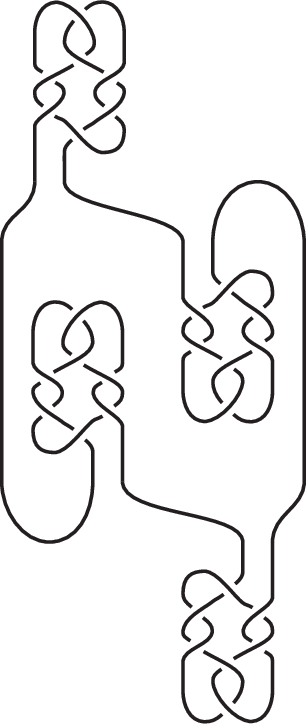
Having seen that the gap between the bridge number of a knot and diagrammatic bridge number in a minimal diagram of can be arbitrarily large for composite knots, we naturally ask whether minimal diagrams of prime knots always realize bridge number. We answer this question in the negative.
Theorem 4.5.
There exists a prime knot with .
Proof.
Let be the knot in Figure 12, and denote the diagram depicted by . Using the algorithm described in [2], we calculated the Wirtinger number of this diagram and found that . Moreover, it is straight-forward to verify that the diagram is adequate and thus crossing number minimizing by [6]. Due to a somewhat lengthy, but standard argument of analyzing the possible intersections between an essential meridional annulus and the various essential surfaces in the exterior , one can show that is prime, see for example Lemma 6.0.29 of [1]. It is similarly straight-forward to show that is an index two cable of the trefoil knot. Hence, by [5], . However, Figure 13, illustrates that . ∎
We believe the method used to construct the knot can be generalized to find other minimal diagrams of prime non-alternating knots , such that and the gap between and grows with the crossing number of . It is interesting to note that there exists a minimal crossing diagram for , given in Figure 13, that realizes bridge number.


References
- [1] Ryan Blair, Bridge number and Conway products, PhD thesis, University of California, Santa Barbara, 2010.
- [2] Ryan Blair, Alexandra Kjuchukova, Roman Velazquez, and Paul Villanueva, Wirtinger systems of generators of knot groups, arXiv:1705.03108.
- [3] Bridge Numbers, https://sites.google.com/a/wisc.edu/alexandra-a-kjuchukova/bridge-numbers, Accessed: 2017-10-31.
- [4] Markus Rost and Heiner Zieschang, Meridional generators and plat presentations of torus links, J. London Math. Soc. (2), 35(3):551–562, 1987.
- [5] Horst Schubert. Über eine numerische Knoteninvariante, Math. Z., 61:245–288, 1954.
- [6] Morwen B. Thistlethwaite, On the Kauffman polynomial of an adequate link, Invent. Math., 93(2):285–296, 1988.