Correlation between Multivariate Datasets, from Inter-Graph Distance computed using Graphical Models Learnt With Uncertainties

Kangrui Wang^??,?? Dalia Chakrabarty^??,??

Abstract

We present a method for simultaneous Bayesian learning of the correlation matrix and graphical model of a multivariate dataset, along with uncertainties in each, to subsequently compute distance between the learnt graphical models of a pair of datasets, using a new metric that approximates an uncertainty-normalised Hellinger distance between the posterior probabilities of the graphical models given the respective dataset; correlation between the pair of datasets is then computed as a corresponding affinity measure. We achieve a closed-form likelihood of the between-columns correlation matrix by marginalising over the between-row matrices. This between-columns correlation is updated first, given the data, and the graph is then updated, given the partial correlation matrix that is computed given the updated correlation, allowing for learning of the 95 $\%$ Highest Probability Density credible regions of the correlation matrix and graphical model of the data. Difference made to the learnt graphical model, by acknowledgement of measurement noise, is demonstrated on a small simulated dataset, while the large human disease-symptom network–with $>8,000$ nodes–is learnt using real data. Data on vino-chemical attributes of Portuguese red and white wine samples are employed to learn with-uncertainty graphical model of each dataset, and subsequently, the distance between these learnt graphical models.

keywords

Graphical models , Random graphs , Inter-graph distance , Hellinger distance , Metropolis-within-Gibbs , Human disease-symptom network

^?? Alan Turing Institute
British Library, 96 Euston Road,
London NW1 2DB,
U.K.
??

^?? Department of Mathematical Sciences
Loughborough University
Loughborough LE11 3TU, U.K.
??

1 Introduction

Graphical models of complex, multivariate datasets, manifest intuitive illustrations of the correlation structures of the data, and are of interest in different disciplines (Whittaker, 2008; Benner et al., 2014; Airoldi, 2007; Carvalho and West, 2007; Bandyopadhyay and Canale, 2016). Much work has been undertaken to study the correlation structure of a multivariate dataset comprising multiple measured values of a vector-valued observable, by modelling the joint probability distribution of a set of such observable values, as matrix-normal (Ni, Stingo and Baladandayuthapani, 2017; Gruber and West, 2016; Wang and West, 2009). In this paper, we simultaneously learn the partial correlation structure and graphical model of a multivariate dataset, while making inference on uncertainties of each, and acknowledge measurement errors in our learning–with the ultimate aim of computing the distance between (posterior probability distributions of) the learnt pair of graphical models of respective datasets. Such distance informs us about the possible independence of the datasets, generated under different environmental conditions. To this effect, we undertake inference with Metropolis-within-Gibbs-based Bayesian inference (Robert and Casella, 2004), on the correlation matrix given the data, and on the graph given the updated correlation.

Objective and comprehensive uncertainties on the Bayesianly learnt graphical model of given multivariate data, are sparsely available in the literature. Such uncertainties can potentially be very useful in informing us about the range of models that describe the partial correlation structure of the data at hand. Madigan and Raftery (1994) discuss a method for computing model uncertainties by averaging over a set of identified models, and they advance ways for the computation of the posterior model probabilities, by taking advantage of the graphical structure, for two classes of considered models, namely, the recursive causal models (Kiiveri, Speed and Carlin, 1984) and the decomposable loglinear models (Goodman, 1970). This method allows them to select the “best models”, while accounting for model uncertainty. Our method on the other hand, provides a direct and well-defined way of learning uncertainties of the graphical model of a given multivariate data. At every update of our learning of the graphical structure of the data, the graph is updated; graphs thus learnt, if identified to lie within an identified range of values of the posterior probability of the graph, comprise the uncertainty-included graphical model of the data (Section 2.3). In addition, our method permits incorporation of measurement errors into the learning of the graphical model, and permits fast learning of large networks (Section 6).

However, we wish to extend such learning to higher-dimensional data, for example, to a dataset that is cuboidally-shaped, given that it comprises multiple measurements of a matrix-valued observable. Hoff (2011); Xu, Yan and Qi. (2012); Wang $\&$ Chakrabarty (https://arxiv.org/abs/1803.04582), advance methods to learn the correlation in high-dimensional data in general. For a rectangularly-shaped multivariate dataset, the pioneering work by Wang and West (2009) allows for the learning of both the between-rows and between-columns covariance matrices, and therefore, of two graphical models. Ni, Stingo and Baladandayuthapani (2017) extend this approach to high-dimensional data. However, a high-dimensional graph showing the correlation structure amongst the multiple components of a general hypercuboidally-shaped dataset, is not easy to visualise or interpret. Instead, in this paper, we treat the high-dimensional data as built of correlated rectangularly-shaped slices, given each of which, the between-columns (partial) correlation structure and graphical model are Bayesianly learnt, along with uncertainties, subsequent to our closed-form marginalisation over all between-rows correlation matrices (in Section 2, unlike in the work of Wang and West (2009)). By invoking the uncertainties learnt in the graphical models, we advance a new inter-graph distance metric (Section 3), based on the Hellinger distance (Matusita, 1953; Banerjee et al., 2015) between the posterior probability densities of the pair of graphical models that are learnt given the respective pair of such rectangularly-shaped data slices. We use a proposed affinity measure to infer on the correlation between the datasets (Section 3.1). For example, by computing the pairwise inter-graph distance between posterior probability densities of each learnt pair of graphs, we can avoid the inadequacy of trying to capture spatial correlations amongst sets of multivariate observations, by “computing partial correlation coefficients and by specifying and fitting more complex graphical models”, as was noted by Guinness et al. (2014). In fact, our method offers the inter-graph distance for two differently sized datasets.

Importantly, we will demonstrate below that it is the learning of uncertainties in graphical models, that allows for the pursuit of the inter-graph distance.

Our learnt graphical model of the given data, comprises a set of random inhomogeneous graphs (Frieze and Karonski, 2016) that lie within the credible regions that we define, where each such graph is a generalisation of a Binomial graph. We do not make inference on the graph (writing its posterior) clique-by-clique, and neither are we reliant on the closed-form nature of the posteriors to sample from. In other words, we do not need to invoke conjugacy to affect our learning–either of the partial correlation structure of the data or of the graphical model. Often, in Bayesian learning of Gaussian undirected graphs, a Hyper-Inverse-Wishart prior is typically imposed on the covariance matrix of the data, as this then allows for a Hyper-Inverse-Wishart posterior of the covariance, which in turn implies that the marginal posterior of of any clique is Inverse-Wishart–a known, closed-form density (Dawid and Lauritzen, 1993; Lauritzen, 1996). Inference is then rendered easier, than when posterior sampling from a non-closed form posterior needs to be undertaken, using numerical techniques such as MCMC. Now, if the graph is not decomposable, and a Hyper-Inverse-Wishart prior is placed on the covariance matrix, the resulting Hyper-Inverse-Wishart joint posterior density that can be factorised into a set of Inverse-Wishart densities, cannot be identified as the clique marginals. Expressed differently, the clique marginals are not closed-form when the graph is not decomposable. However, this is not a worry in our learning, i.e. we can undertake our learning irrespective of the validity of decomposability.

This paper is organised as follows. The following section deliberates upon the methodology that we advance, including the closed-form likelihood of the between-column correlation matrix of the data at hand, and definition of the uncertainties on the learnt graphical model. The method of computing the inter-graph distance that invokes such learnt uncertainties, is then discussed in Section 3. Section 4 presents the emiprical illustration on 2 real datasets, with the distance between the learnt, with-uncertainty graphical models of these 2 data, discussed in Section 5. In Section 6, we learn the graphical model of a real, highly multivariate, dataset, namely the human disease-phenotype dataset, and compare our results with those reported earlier (Hoehndorf, Schofield and Gkoutos, 2015). The paper is rounded up with a section that summarises the main findings and the conclusions. The attached Supplementary Materials elaborate on certain aspects of our work. This includes comparison of results obtained by using our method with existing and independently obtained results, relevant to a pair of real datasets that we illustrate our methodology on in this paper (Sections 4 and 6 of the Supplementary Material), and importantly, detailed model checking is discussed in Section 2 of the Supplementary Material.

2 Learning correlation matrix and graphical model given data, using Metropolis-within-Gibbs

Let $\boldsymbol{X}\in{\cal X}\subseteq{\mathbb{R}}^{p}$ be a $p$ -dimensional observed vector, with $\boldsymbol{X}=(X_{1},\ldots,X_{p})^{T}$ . Let there be $n$ measurements of $X_{j}$ , $j=1,\ldots,p$ , so that the $n\times p$ -dimensional matrix ${\bf D}=[x_{ij}]_{i=1;j=1}^{n;p}$ is the data that comprises $n$ measurements of the $p$ -dimensional observable $\boldsymbol{X}$ . Let the $i$ -th realisation of $\boldsymbol{X}$ be $\boldsymbol{x}_{i}$ , $i=1,\ldots,n$ . We standardise the variable $X_{j}$ ( $j=1,\ldots,p$ ) by its empirical mean and standard deviation, into $Z_{j}$ , s.t. the standardised version ${\bf D}_{S}$ of data ${\bf D}$ comprises $n$ measurements of the $p$ -dimensional vector $\boldsymbol{Z}=(Z_{1},\ldots,Z_{p})^{T}$ . Thus, $z_{ij}=\displaystyle{\frac{x_{ij}-\bar{x}_{j}}{\Upsilon_{j}}}$ , where $\bar{x}_{j}:=\displaystyle{\frac{\sum\limits_{i=1}^{n}x_{ij}}{n}}$ and $\Upsilon_{j}^{2}:=\displaystyle{\frac{\sum\limits_{i=1}^{n}x_{ij}^{2}}{n}-\left(\frac{\sum\limits_{i=1}^{n}x_{ij}}{n}\right)^{2}}$ . The $n\times p$ -dimensional matrix ${\bf D}_{S}=[z_{ij}]$ . Then we model the joint probability of a set of measurements of $\boldsymbol{Z}$ , (such as the set of $n$ that comprises the standardised data ${\bf D}_{S}$ ), to be matrix-normal with zero-mean, i.e.

\{\boldsymbol{z}_{1},\ldots,\boldsymbol{z}_{n}\}\sim{\cal MN}({\bf 0},\boldsymbol{\Sigma}_{R}^{(S)},\boldsymbol{\Sigma}_{C}^{(S)}),

i.e. the likelihood of the covariance matrices $\boldsymbol{\Sigma}_{R}^{(S)}$ and $\boldsymbol{\Sigma}_{C}^{(S)}$ , given data ${\bf D}_{S}$ , is matrix-normal:

\ell(\boldsymbol{\Sigma}_{R}^{(S)},\boldsymbol{\Sigma}_{C}^{(S)}|{\bf D}_{S})=\displaystyle{\frac{1}{(2\pi)^{\frac{np}{2}}|\boldsymbol{\Sigma}_{C}^{(S)}|^{\frac{p}{2}}|\boldsymbol{\Sigma}_{R}^{(S)}|^{\frac{n}{2}}}\times\exp\left[-\frac{1}{2}tr\left\{(\boldsymbol{\Sigma}_{R}^{(S)})^{-1}{\bf D}_{S}(\boldsymbol{\Sigma}_{C}^{(S)})^{-1}({\bf D}_{S})^{T}\right\}\right]},

(2.1)

Here $\boldsymbol{\Sigma}_{R}^{(S)}$ generates the covariance between the standardised variables $\boldsymbol{Z}_{i}$ and $\boldsymbol{Z}_{i^{/}}$ , $i,i^{/}=1,\ldots,n$ , (while $\boldsymbol{\Sigma}_{R}$ generates the covariance between $\boldsymbol{X}_{i}$ and $\boldsymbol{X}_{i^{/}}$ ). In other words, $\boldsymbol{\Sigma}_{R}^{(S)}$ generates the correlation between rows of the standardised data set ${\bf D}_{S}$ . Similarly, $\boldsymbol{\Sigma}_{C}^{(S)}$ generates the correlation between columns of ${\bf D}_{S}$ .

Theorem 2.1.

The joint posterior probability density of the correlation matrices $\boldsymbol{\Sigma}_{C}^{(S)},\boldsymbol{\Sigma}_{R}^{(S)}$ , given the standardised data ${\bf D}_{S}$ is

\left[\boldsymbol{\Sigma}_{C}^{(S)},\boldsymbol{\Sigma}_{R}^{(S)}|{\bf D}_{S}\right]\propto\ell(\boldsymbol{\Sigma}_{R}^{(S)},\boldsymbol{\Sigma}_{C}^{(S)}|{\bf D}_{S})\left[\boldsymbol{\Sigma}_{C}^{(S)},\boldsymbol{\Sigma}_{R}^{(S)}\right],

where $\ell(\boldsymbol{\Sigma}_{R}^{(S)},\boldsymbol{\Sigma}_{C}^{(S)}|{\bf D}_{S})$ is the likelihood of $\boldsymbol{\Sigma}_{R}^{(S)},\boldsymbol{\Sigma}_{C}^{(S)}$ given data ${\bf D}_{S}$ . This can be marginalised over the $n\times n$ -dimensional between-rows’ correlation $\boldsymbol{\Sigma}_{R}^{(S)}$ , to yield

[\boldsymbol{\Sigma}_{C}^{(S)}|{\bf D}_{S}]\propto\displaystyle{\frac{1}{c\left(\boldsymbol{\Sigma}_{C}^{(S)}\right){\Big|}\boldsymbol{\Sigma}_{C}^{(S)}{\Big|}^{p/2}{\Big|}{\bf D}_{S}(\boldsymbol{\Sigma}_{C}^{(S)})^{-1}({\bf D}_{S})^{T}{\Big|}^{\frac{n+1}{2}}}},

where the prior on $\boldsymbol{\Sigma}_{C}^{(S)}$ is uniform; prior on $\boldsymbol{\Sigma}_{R}^{(S)}$ is the non-informative $\pi_{0}(\boldsymbol{\Sigma}_{R}^{(S)})={\Big|}\boldsymbol{\Sigma}_{R}^{(S)}{\Big|}^{\alpha}$ , $\alpha=\displaystyle{-\frac{n}{2}-1}$ , and $\boldsymbol{\Sigma}_{C}^{(S)}$ is assumed invertible. Here, $c\left(\boldsymbol{\Sigma}_{C}^{(S)}\right)$ is a function of $\boldsymbol{\Sigma}_{C}^{(S)}$ that normalises the likelihood.

Proof.

The joint posterior probability density of $\boldsymbol{\Sigma}_{C}^{(S)},\boldsymbol{\Sigma}_{R}^{(S)}$ , given data ${\bf D}_{S}$ :

$\displaystyle\left[\boldsymbol{\Sigma}_{C}^{(S)},\boldsymbol{\Sigma}_{R}^{(S)}\|{\bf D}_{S}\right]$	$\displaystyle\propto$	$\displaystyle\displaystyle{\ell\left(\boldsymbol{\Sigma}_{R}^{(S)},\boldsymbol{\Sigma}_{C}^{(S)}\|{\bf D}_{S}\right)\left[\boldsymbol{\Sigma}_{C}^{(S)},\boldsymbol{\Sigma}_{R}^{(S)}\right],\quad{\mbox{i.e.}}}$
$\displaystyle\left[\boldsymbol{\Sigma}_{C}^{(S)},\boldsymbol{\Sigma}_{R}^{(S)}\|{\bf D}_{S}\right]$	$\displaystyle\propto$	$\displaystyle\displaystyle{\frac{1}{(2\pi)^{\frac{np}{2}}{\Big\|}\boldsymbol{\Sigma}_{C}^{(S)}{\Big\|}^{\frac{p}{2}}{\Big\|}\boldsymbol{\Sigma}_{R}^{(S)}{\Big\|}^{\frac{n}{2}}}\times}$
		$\displaystyle\displaystyle{\exp\left[-\frac{1}{2}tr\left\{(\boldsymbol{\Sigma}_{R}^{(S)})^{-1}({\bf D}_{S})(\boldsymbol{\Sigma}_{C}^{(S)})^{-1}({\bf D}_{S})^{T}\right\}\right]{\Big\|\boldsymbol{\Sigma}_{R}^{(S)}\Big\|^{-\frac{n}{2}-1}}},$

using the likelihood from Equation 2.1; using prior on $\boldsymbol{\Sigma}_{R}^{(S)}$ to be $\pi_{0}(\boldsymbol{\Sigma}_{R}^{(S)})={\Big|}\boldsymbol{\Sigma}_{R}^{(S)}{\Big|}^{\alpha}$ where $\alpha=\displaystyle{-\frac{n}{2}-1}$ ; using prior on $\boldsymbol{\Sigma}_{C}^{(S)}$ to be uniform.

Marginalising $\boldsymbol{\Sigma}_{R}^{(S)}$ out from the joint posterior $\left[\boldsymbol{\Sigma}_{C}^{(S)},\boldsymbol{\Sigma}_{R}^{(S)}|{\bf D}_{S}\right]$ , we get:

\left[\boldsymbol{\Sigma}_{C}^{(S)}|{\bf D}_{S}\right]\propto

\displaystyle{\frac{1}{{\Big|}\boldsymbol{\Sigma}_{C}^{(S)}{\Big|}^{\frac{p}{2}}}\times}\displaystyle{\int\limits_{{\cal R}}\frac{1}{{\Big|}\boldsymbol{\Sigma}_{R}^{(S)}{\Big|}^{\frac{n}{2}}}{\Big|}\boldsymbol{\Sigma}_{R}^{(S)}{\Big|}^{-\frac{n}{2}-1}\times\exp\left[-\frac{1}{2}tr\left\{(\boldsymbol{\Sigma}_{R}^{(S)})^{-1}{\bf D}_{S}(\boldsymbol{\Sigma}_{C}^{(S)})^{-1}({\bf D}_{S})^{T}\right\}\right]d(\boldsymbol{\Sigma}_{R}^{(S)})}

(2.3)

Here $\boldsymbol{\Sigma}_{R}^{(S)}\in{\cal R}\subseteq{\mathbb{R}}^{(n\times n)}$ . Now,

–

let $\boldsymbol{Y}:=(\boldsymbol{\Sigma}_{R}^{(S)})^{-1}$ . Then $d(\boldsymbol{\Sigma}_{R}^{(S)})=|\boldsymbol{Y}|^{-(n+1)}d\boldsymbol{Y}$ (Mathai and G.Pederzoli, 1997),
–

let $\boldsymbol{V}^{-1}:={\bf D}_{S}(\boldsymbol{\Sigma}_{C}^{(S)})^{-1}({\bf D}_{S})^{T}$ , $\Longrightarrow tr\left[(\boldsymbol{\Sigma}_{R}^{(S)})^{-1}{\bf D}_{S}(\boldsymbol{\Sigma}_{C}^{(S)})^{-1}({\bf D}_{S})^{T}\right]\equiv tr\left[\boldsymbol{V}^{-1}\boldsymbol{Y}\right]$ (using commutativeness of trace),

so that in Equation 2.3, we get

\displaystyle\left[\boldsymbol{\Sigma}_{C}^{(S)}|{\bf D}_{S}\right]

\displaystyle\propto

\displaystyle\displaystyle{\frac{1}{{\Big|}\boldsymbol{\Sigma}_{C}^{(S)}{\Big|}^{\frac{p}{2}}}\int\limits_{{\cal R}}{|\boldsymbol{Y}|^{\frac{n}{2}}}|\boldsymbol{Y}|^{\frac{n}{2}+1}\times\exp\left[-\frac{1}{2}tr\left\{\boldsymbol{V}^{-1}\boldsymbol{Y}\right\}\right]|\boldsymbol{Y}|^{-(n+1)}d\boldsymbol{Y}}.

The integral in the RHS of Equation represents the unnormalised Wishart $pdf$ $W_{n}(\boldsymbol{V},q)$ , over all values of the random matrix $\boldsymbol{Y}$ , where the scale matrix and degrees of freedom of this $pdf$ are $\boldsymbol{V}$ and $q=n+1$ respectively, i.e. $q>n-1$ .
Thus, integral in the RHS of Equation is the integral of the unnormalised $pdf$ of $\boldsymbol{Y}\sim W_{n}(\boldsymbol{V},q)$ , over the full support of $\boldsymbol{Y}\left(\equiv\left(\boldsymbol{\Sigma}_{R}^{(S)}\right)^{-1}\right)$ ,
i.e. the integral in the RHS of Equation is the normalisation of this $pdf$ :

2^{\frac{qn}{2}}\Gamma_{n}\left(\frac{q}{2}\right)|\boldsymbol{V}|^{\frac{q}{2}}\equiv

2^{\frac{(n+1)(n)}{2}}\Gamma_{n}\left(\frac{n+1}{2}\right){\Big|}\left({\bf D}_{S}(\boldsymbol{\Sigma}_{C}^{(S)})^{-1}({\bf D}_{S})^{T}\right)^{-1}{\Big|}^{\frac{n+1}{2}},

i.e. integral on RHS of Equation is proportional to ${\Big|}\left({\bf D}_{S}(\boldsymbol{\Sigma}_{C}^{(S)})^{-1}({\bf D}_{S})^{T}\right)^{-1}{\Big|}^{\frac{n+1}{2}},\quad{\mbox{i.e.}}$

\left[\boldsymbol{\Sigma}_{C}^{(S)}|{\bf D}_{S}\right]\propto\displaystyle{\frac{1}{{\Big|}\boldsymbol{\Sigma}_{C}^{(S)}{\Big|}^{\frac{p}{2}}}{\Big|}\left({\bf D}_{S}(\boldsymbol{\Sigma}_{C}^{(S)})^{-1}({\bf D}_{S})^{T}\right)^{-1}{\Big|}^{\frac{n+1}{2}}}

(2.5)

Now, if ${\bf D}_{S}(\boldsymbol{\Sigma}_{C}^{(S)})^{-1}({\bf D}_{S})^{T}$ is invertible, ${\Big|}\left({\bf D}_{S}(\boldsymbol{\Sigma}_{C}^{(S)})^{-1}({\bf D}_{S})^{T}\right)^{-1}{\Big|}^{\cdot}={\Big|}{\bf D}_{S}(\boldsymbol{\Sigma}_{C}^{(S)})^{-1}({\bf D}_{S})^{T}{\Big|}^{-{\cdot}}$ .

–

It is given that $\boldsymbol{\Sigma}_{C}^{(S)}$ is invertible, i.e. $\left(\boldsymbol{\Sigma}_{C}^{(S)}\right)^{-1}$ exists.
–

The original dataset is examined to discard rows that are linear transformations of each other, leading to data matrix ${\bf D}_{S}$ , no two rows of which are linear transformations of each other

$\Longrightarrow$ ${\bf D}_{S}(\boldsymbol{\Sigma}_{C}^{(S)})^{-1}({\bf D}_{S})^{T}$ is positive definite, i.e. ${\bf D}_{S}(\boldsymbol{\Sigma}_{C}^{(S)})^{-1}({\bf D}_{S})^{T}$ is invertible,
$\Longrightarrow$ ${\Big|}\left({\bf D}_{S}(\boldsymbol{\Sigma}_{C}^{(S)})^{-1}({\bf D}_{S})^{T}\right)^{-1}{\Big|}^{(n+1)/2}={\Big|}{\bf D}_{S}(\boldsymbol{\Sigma}_{C}^{(S)})^{-1}({\bf D}_{S})^{T}{\Big|}^{-{(n+1)/2}}$ .

Using this in Equation 2.5:

\left[\boldsymbol{\Sigma}_{C}^{(S)}|{\bf D}_{S}\right]\propto{\Big|}{\boldsymbol{\Sigma}}_{C}^{(S)}{\Big|}^{-{p/2}}{\Big|}{\bf D}_{S}(\boldsymbol{\Sigma}_{C}^{(S)})^{-1}({\bf D}_{S})^{T}{\Big|}^{-{(n+1)/2}}.

(2.6)

This posterior of the between-columns correlation matrix $\boldsymbol{\Sigma}_{C}^{(S)}$ given data ${\bf D}_{S}$ , is normalised over all possible datasets, where the possible datasets abide by a column-correlation matrix of $\boldsymbol{\Sigma}_{C}^{(S)}$ , as:

c\left(\boldsymbol{\Sigma}_{C}^{(S)}\right)=\displaystyle{\int\limits_{\cal Z}\ldots\int\limits_{\cal Z}\frac{1}{{\Big|}\left({\bf D}^{/}(\boldsymbol{\Sigma}_{C}^{(S)})^{-1}({\bf D}^{/})^{T}\right){\Big|}^{\frac{n^{/}+1}{2}}}dz_{11}^{/}dz_{11}^{/}\ldots dz_{n^{/}p}^{/}},

(2.7)

where ${\bf D}^{/}=[z_{ij}^{/}]_{i=1;j=1}^{i=n^{/};j=p}$ is a dataset with $n^{/}$ rows and $p$ columns, comprising values of random standardised variables $Z_{ij}^{/}\in{\cal Z}$ , simulated to bear between-column correlation matrix of $\boldsymbol{\Sigma}_{C}^{(S)}$ , s.t. ${\bf D}^{/}(\boldsymbol{\Sigma}_{C}^{(S)})^{-1}({\bf D}^{/})^{T}$ is positive definite $\forall{\bf D}^{/}\in{\cal D}$ . Choosing the same number of rows for all choices of the random data matrix ${\bf D}^{/}$ , i.e. for a constant $n^{/}$ , ${\cal D}\subseteq{\mathbb{R}}^{(n^{/}\times p)}$ . Then $c\left(\boldsymbol{\Sigma}_{C}^{(S)}\right)>0$ for any $\boldsymbol{\Sigma}_{C}^{(S)}$ .

Using this normalisation on the posterior of $\boldsymbol{\Sigma}_{C}^{(S)}$ given ${\bf D}_{S}$ , in Equation 2.6 we get

\pi\left(\boldsymbol{\Sigma}_{C}^{(S)}|{\bf D}_{S}\right)=\displaystyle{\frac{1}{c\left(\boldsymbol{\Sigma}_{C}^{(S)}\right){\Big|}\boldsymbol{\Sigma}_{C}^{(S)}{\Big|}^{\frac{p}{2}}}\frac{1}{{\Big|}\left({\bf D}_{S}(\boldsymbol{\Sigma}_{C}^{(S)})^{-1}({\bf D}_{S})^{T}\right){\Big|}^{\frac{n+1}{2}}}},

(2.8)

where $c\left(\boldsymbol{\Sigma}_{C}^{(S)}\right)>0$ is defined in Equation 2.7. ∎

Proposition 2.1.

An estimator of the normalisation ${\hat{c}}\left(\boldsymbol{\Sigma}_{C}^{(S)}\right)$ of the posterior $\left[\boldsymbol{\Sigma}_{C}^{(S)}|{\bf D}_{S}\right]$ , given in Equation 2.7 is

{\hat{c}}\left(\boldsymbol{\Sigma}_{C}^{(S)}\right)=\displaystyle{{\mathbb{E}}_{Z^{/}_{n^{/}p}}\left[\ldots\left[{\mathbb{E}}_{Z^{/}_{11}}\left[\displaystyle{\frac{1}{{\Big|}\left({\bf D}^{/}(\boldsymbol{\Sigma}_{C}^{(S)})^{-1}({\bf D}^{/})^{T}\right){\Big|}^{\frac{n^{/}+1}{2}}}}\right]\right]\ldots\right]}.

We substitute this difficult, sequential computing of expectations w.r.t. distribution of each element of ${\bf D}^{/}$ , by computation of the expectation w.r.t. the block ${\bf D}^{/}$ of these elements, where ${\bf D}^{/}$ abides by a column-correlation of $\boldsymbol{\Sigma}_{C}^{(S)}$ , i.e., we compute

{\hat{c}}^{/}\left(\boldsymbol{\Sigma}_{C}^{(S)}\right)=\displaystyle{{\mathbb{E}}_{{\bf D}^{/}_{S}}\left[\displaystyle{\frac{1}{{\Big|}\left({\bf D}^{/}(\boldsymbol{\Sigma}_{C}^{(S)})^{-1}({\bf D}^{/})^{T}\right){\Big|}^{\frac{n^{/}+1}{2}}}}\right]}.

We consider a between-columns correlation matrix $\boldsymbol{\Sigma}_{t}$ , and the sample of $k$ number of $n^{/}\times p$ -dimensional data sets $\{{\bf D}_{1}^{t/},\ldots,{\bf D}_{K}^{t/}\}$ , s.t. ${\bf D}_{k}^{t/}(\boldsymbol{\Sigma}_{t})^{-1}({\bf D}_{k}^{t/})^{T}$ is positive definite $\forall k=1,\ldots,K$ , at each $t$ , the estimator of ${\hat{c}}^{/}\left(\boldsymbol{\Sigma}_{t}\right)$ is

{\hat{c}}_{t}:=\displaystyle{\frac{1}{K}{\sum\limits_{k=1}^{K}\frac{1}{{\Big|}\left({\bf D}_{k}^{t/}(\boldsymbol{\Sigma}_{t})^{-1}({\bf D}_{k}^{t/})^{T}\right){\Big|}^{\frac{n^{/}+1}{2}}}}}.

(2.9)

Generation of a randomly sampled $n^{/}\times p$ -sized data set ${\bf D}_{k}^{t/}$ , with column correlation $\boldsymbol{\Sigma}_{t}$ , is undertaken.

2.1 Learning the graphical model

We perform Bayesian learning of the inhomogeneous, Generalised Binomial random graph ${\mathbb{G}}(p,\boldsymbol{R})$ , given the learnt $p\times p$ -dimensional, between-columns correlation matrix $\boldsymbol{\Sigma}_{C}^{(S)}$ , of the standardised data set ${\bf D}_{S}:=(\boldsymbol{Z}_{1},\vdots,\ldots,\vdots,\boldsymbol{Z}_{p})^{T}$ . Here, the graph ${\mathbb{G}}(p,\boldsymbol{R})$ , has the vertex set $\boldsymbol{V}$ and the between-columns partial correlation matrix $\boldsymbol{R}$ of data ${\bf D}_{S}$ , where $\boldsymbol{R}=[R_{ij}]$ , s.t. $R_{ij}$ takes the value $\rho_{ij}$ , $i\neq j$ , and $\rho_{ii}=1$ . The vertex set is $\boldsymbol{V}=\{1,\ldots,p\}$ s.t. vertices $i,j\in\boldsymbol{V},\>i\neq j$ , are joined by the edge $G_{ij}$ that is a random binary variable taking values of $g_{ij}$ , where $g_{ij}$ is either 1 or 0, and is the $ij$ -th element of the edge matrix $\boldsymbol{G}=[G_{ij}]$ .

Given a learnt value of the between-columns correlation matrix $\boldsymbol{\Sigma}_{C}^{(S)}$ , to compute the value $\rho_{ij}$ of the partial correlation variable $R_{ij}$ , we first invert $\boldsymbol{\Sigma}_{C}^{(S)}$ to yield: $\boldsymbol{\Psi}:=\left(\boldsymbol{\Sigma}_{C}^{(S)}\right)^{-1};\>\boldsymbol{\Psi}=[\psi_{ij}]$ , s.t.

R_{ij}=-\displaystyle{\frac{\psi_{ij}}{\sqrt{\psi_{ii}\psi_{jj}}}},\quad i\neq j,

(2.10)

and $\rho_{ii}=1$ for $i=j$ .

The posterior probability density of the graph ${\mathbb{G}}(p,\boldsymbol{R})$ defined for the edge matrix $\boldsymbol{G}$ , is given as

\pi(G_{11},G_{12},\ldots G_{p\>p-1}|\boldsymbol{R})\propto\ell(G_{11},G_{12},\ldots G_{p\>p-1}|\boldsymbol{R})\>\pi_{0}(G_{11},G_{12},\ldots G_{p\>p-1}),

where $\pi_{0}(G_{11},G_{12},\ldots G_{p\>p-1})$ is the prior probability density on the edge parameters $\{G_{ij}\}_{i\neq j;i,j=1}^{p}$ . We choose a prior on $G_{ij}$ that is $Bernoulli(0.5)$ , i.e. $\pi_{0}(G_{11},G_{12},\ldots G_{p\>p-1})=\displaystyle{\prod\limits_{i,j=1;i\neq j}^{p}0.5^{g_{ij}}0.5^{1-g_{ij}}}$ ; thus, the prior is independent of the edge parameters. In applications marked by more information, we can resort to stronger priors.

$\ell(G_{12},\ldots,G_{1p},G_{23},\ldots,G_{2p},G_{34},\ldots,G_{p\>p-1}|\boldsymbol{R})$ is the likelihood of the edge parameters, given the partial correlation matrix $\boldsymbol{R}$ (that is itself computed using the between-columns correlation matrix $\boldsymbol{\Sigma}_{C}^{(S)}$ , learnt given ${\bf D}_{S}$ , (see Equation 2.8). We choose to define this likelihood as a function of the (squared) Euclidean distance between the “observation”, i.e. the value of $R_{ij}$ , and the unknown parameter $G_{ij}$ , with the squared distance normalised by a squared scale length, or variance parameter $\sigma_{ij}^{2}$ , for all relevant pairs of nodes. Thus, the unknown parameters in the model are the edge and variance parameters; in light of these newly introduced variance parameters, we rewrite our likelihood as $\ell(G_{12},\ldots,G_{1p},G_{23},\ldots,G_{2p},G_{34},\ldots,G_{p\>p-1},$
$\sigma_{12}^{2},\ldots,\sigma_{1p}^{2},\sigma_{23}^{2},\ldots,\sigma_{2p}^{2},\sigma_{34}^{2},\ldots,\sigma_{p\>p-1}^{2}|\boldsymbol{R})$ . Then the constraints on the likelihood function suggest that likelihood increases (decreases) as distance between $R_{ij}$ and $G_{ij}$ decreases (increases), and likelihood invariant to change of sign of $R_{ij}-G_{ij}$ . Given these constraints, we model our likelihood of the edge and variance parameters, given $\boldsymbol{R}$ as

\ell\left(G_{12},\ldots,G_{1p},G_{23},\ldots,G_{2p},\ldots,G_{p\>p-1},\sigma_{12}^{2},\ldots,\sigma_{1p}^{2},\sigma_{23}^{2},\ldots,\sigma_{2p}^{2},\ldots,\sigma_{p\>p-1}^{2}|\boldsymbol{R}\right)=

\displaystyle{\prod\limits_{i\neq j;i,j=1}^{p}\frac{1}{\sqrt{2\pi\sigma_{ij}^{2}}}\exp\left[-\frac{\left(G_{ij}-R_{ij}\right)^{2}}{2\sigma_{ij}^{2}}\right]},

(2.11)

where the variance parameters $\{\sigma_{ij}^{2}\}_{i\neq j;i,j=1}^{p}$ are indeed hyperparameters that are also learnt from the data; these variance parameters have uniform prior probabilities imposed on them.

2.2 Inference using Metropolis-within-Gibbs

Equation 2.8 gives the posterior probability density of correlation matrix ${\boldsymbol{\Sigma}}_{C}^{(S)}$ , given data ${\bf D}_{S}$ . In our Metropolis-within-Gibbs based inference, we update ${\boldsymbol{\Sigma}}_{C}^{(S)}$ –at which the partial correlation matrix $\boldsymbol{R}$ is computed. Given this updated $\boldsymbol{R}$ , we then update the graph ${\mathbb{G}}(p,\boldsymbol{R})$ . The graphical model comprising the credible-region defining set of random Binomial graphs $\{{\mathbb{G}}(p,\boldsymbol{R})\}$ is thus learnt, where the vertex set of each graph in this set is fixed as $\boldsymbol{V}$ ; the “credible region” in question is defined below in Section 2.3.

In our learning of the $p\times p$ -dimensional between-columns correlation matrix ${\boldsymbol{\Sigma}}_{C}^{(S)}$ , the $\displaystyle{\frac{p^{2}-p}{2}}$ non-diagonal elements of the upper (or lower) triangle are learnt, i.e. the parameters $S_{12},S_{13},\ldots,S_{1p},S_{23},\ldots,S_{p-1\>p}$ are learnt. In the $t$ -th iteration of our inference, $S_{ij}$ is proposed from a Truncated Normal density that is left truncated at -1 and right truncated at 1, as $s_{ij}^{(t*)}\sim{{\cal TN}}(s_{ij}^{(t*)};s_{ij}^{(t-1)},v_{ij},-1,1),\quad,\forall\>i,j=1,\ldots,p;\>i\neq j,$ where $v_{ij}=v_{0}\forall\>i,j$ is the experimentally chosen variance, and the proposal mean is the current value $s_{ij}^{(t-1)}$ of $S_{ij}$ at the end of the $t-1$ -th iteration. At the 2nd block of the $t$ -th iteration, the graph variable ${\mathbb{G}}(p,\boldsymbol{R})$ is updated, given the current partial correlation matrix $\boldsymbol{R}_{t}$ , s.t. the proposed edge variable connecting the $i$ -th to the $j$ -th vertex is $g_{ij}^{(t\star)}\sim{Bernoulli}(g_{ij}^{(t\star)};\rho_{ij}^{(t)})$ , and the $ij$ -th proposed variance parameter is $\sigma_{ij}^{(t\star)}\sim{\cal N}(\sigma_{ij}^{(t\star)};\sigma_{ij}^{(t-1)},w_{ij}^{2})$ , where $w_{ij}^{2}$ are the experimentally chosen variance and the mean is the current value of $\sigma_{ij}$ . (Details in Section 1 of the Supplementary Material).

As suggested in Equation 2.8, the correlation learning involves computing $\left({\boldsymbol{\Sigma}}_{C}^{(S)}\right)^{-1}$ , $|{\boldsymbol{\Sigma}}_{C}^{(S)}|$ and $|{\bf D}_{S}\left({\boldsymbol{\Sigma}}_{C}^{(S)}\right)^{-1}\left({\bf D}_{S}\right)^{T}|$ , in every iteration. This calls for Cholesky decomposition of $\boldsymbol{\Sigma}_{C}^{(S)}$ as $\boldsymbol{L}_{C}^{(S)}(\boldsymbol{L}_{C}^{(S)})^{T}$ , and of ${\bf D}_{S}\left({\boldsymbol{\Sigma}}_{C}^{(S)}\right)^{-1}\left({\bf D}_{S}\right)^{T}$ , into the (lower) triangular matrix $\boldsymbol{L}$ and $\boldsymbol{L}^{T}$ , while implementing ridge adjustment (Wothke, 1993). The latter computation follows the inversion of $\boldsymbol{\Sigma}_{C}^{(S)}$ into $(\boldsymbol{\Sigma}_{C}^{(S)})^{-1}$ , which is undertaken using a forward substitution algorithm. (Details in Section 7 of the Supplementary Material).

2.3 Defining the 95 $\%$ HPD credible regions on the random graph variable, and the learnt graphical model

We perform Bayesian inference on the random graph variable ${\mathbb{G}}(p,\boldsymbol{R})$ , leading to one sampled graph at the end of each of the $N+1$ iterations of our inference scheme (Metropolis-within-Gibbs). In order to acknowledge uncertainties in the Bayesian learning of the sought graphical model, we need to include in its definition, only those graphs–sampled post-burnin–that lie within an identified 95 $\%$ HPD credible region. We define the fraction $N_{ij}$ of the post-burnin number $N_{post}$ of iterations (where $N_{post}<N+1$ ), in which the $ij$ -th edge exists, i.e. $G_{ij}$ takes the value 1, $\forall\>i,j=1,2,\ldots,p,\>i\neq j$ . Thus, variable $N_{ij}$ takes the value

n_{ij}:=\displaystyle{\frac{\sum\limits_{t=N-N_{post}+1}^{N}g_{ij}^{(t)}}{N_{post}}},\quad i<j;\>i,j=1,\ldots,p,

(2.12)

where the Bernoulli edge-variable $G_{ij}=g_{ij}^{(t)}$ in the $t$ -th iteration. Then $N_{ij}$ is the fractional number of sampled graphs, in which an edge exists between vertices $i$ and $j$ . This leads us to interpret $\{N_{ij}\}_{i,j\in V;\>i<j}$ as carrying information about the uncertainty in the graph learnt given data ${\bf D}_{S}$ ; in particular, $n_{ij}$ approximates the probability of existence of the edge between the $i$ -th and $j$ -th nodes in the graphical model of the data at hand. Indeed the $N_{ij}$ parameters are functions of the partial correlation matrix $\boldsymbol{R}$ that is learnt given this data, but for the sake of notational brevity, we do not include this explicit $\boldsymbol{R}$ dependence in our notation to denote the edge probability parameters.

So we view the set $\{{\mathbb{G}}(p,\boldsymbol{R}_{t})\}_{t=N-N_{post}+1}^{N}$ of graphs on vertex set $\boldsymbol{V}=\{1,\ldots,p\}$ and edge matrix $\boldsymbol{G}_{t}$ in the $t$ -th iteration, that is updated given the current partial correlation matrix $\boldsymbol{R}_{t}$ in the $t$ -th iteration, equivalently as the post-burnin sample
$\{g^{(t)}_{12},g^{(t)}_{13},\ldots,g^{(t)}_{1p},g^{(t)}_{23},\ldots,g^{(t)}_{p\>p-1}\}_{t=N-N_{post}+1}^{N}$ of edge parameters. We include only those edge parameters in our defined 95 $\%$ HPD credible region, that occur with probability $\geq 0.05$ in this sample. In other words, only for $ij$ pairs s.t. $N_{ij}\geq 0.05$ , define the $g_{ij}$ parameters included in the set that comprises the 95 $\%$ HPD credible region on the edge parameters, in our definition. Indeed, the graphical model of the data is then the set of those graphs on vertex set $\boldsymbol{V}=\{1,\ldots,p\}$ , the existing edges of which are those $G_{ij}$ parameters that lie within this defined 95 $\%$ HPD credible region.

Definition 2.1.

The graphical model of data ${\bf D}_{S}$ for which the between-column partial correlation matrix is $\boldsymbol{R}$ , is the $\boldsymbol{R}$ -dependent set or family $\displaystyle{{\cal G}_{p,{\boldsymbol{\Phi}}(\boldsymbol{R})}}$ of all inhomogeneous Binomial graphs ${\mathbb{G}}(p,\boldsymbol{R})$ , the edge probabilities in which are given by the matrix $\boldsymbol{\Phi}(\boldsymbol{R})=[\phi_{ij}(R_{ij})]$ , s.t. probability of the edge between the $i$ -th and $j$ -th nodes ( $i\neq j;\>i,j\in V$ ) is

\phi_{ij}(R_{ij})=\left[H(n_{ij}-0.05)\right]n_{ij}.

(2.13)

Here, $n_{ij}$ is the value of the parameter $N_{ij}$ defined in Equation 2.12, and $H(\cdot)$ is the Heaviside function (Duff and Naylor, 1966) where the Heaviside or step-function of $A\in{\mathbb{R}}$ is

	$\displaystyle H(a)$	$\displaystyle=$	$\displaystyle 1\quad{\mbox{if}}\quad a\geq 0$
		$\displaystyle=$	$\displaystyle 0\quad{\mbox{if}}\quad a<0.$

Only edges with non-zero edge probability $\phi_{ij}(R_{ij})$ , are marked on the learnt graphical model, and the corresponding value of $N_{ij}$ is written next to each such marked edge. Then by this definition, any graph ${\mathbb{G}}(p,\boldsymbol{R})\in\displaystyle{{\cal G}_{p,{\boldsymbol{\Phi}}(\boldsymbol{R})}}$ is sampled from within the 95 $\%$ HPD credible region on inhomogeneous random Binomial graphs given the partial correlation matrix $\boldsymbol{R}$ of the data.

Thus, in our approach, the binary edge parameter $G_{ij}$ between the $i$ -th and $j$ -th nodes, takes the value 1 (i.e. the edge exists), with a learnt probability–in fact, we learn the joint posterior of all $G_{ij}$ parameters given the learnt correlation structure of the data, while acknowledging the propagation of uncertainties in our learning of the correlation given the data, into our learning of the distribution of the $G_{ij}$ parameters given this learnt partial correlation matrix $\boldsymbol{R}$ . A summary of this learnt distribution is then the edge probability parameter $\phi_{ij}(R_{ij})$ , the value of which is marked on the visualisation of the graphical model of the data against the edge between the $i$ -th and $j$ -th nodes, as long as $\phi_{ij}(R_{ij})>0$ , i.e. $n_{ij}\geq 0.05$ ; $i\neq j;\>i,j\in\boldsymbol{V}$ . In other words, only edges occurring with posterior probabilities in excess of 5 $\%$ are included in this graphical model.

3 Uncertainties in learnt graphical models help compute inter-graph distance

We compute the distance between the graphical models of two multivariate datasets ${\bf D}_{1}$ and ${\bf D}_{2}$ of disparate sizes ( $n_{1}$ and $n_{2}$ respectively), to compute the correlation between them; in effect, the exercise can address the possible independence of the $pdf$ s that the two datasets are sampled from. This is of course a hard question to address when the data comprise measurements of a high-dimensional vector-valued observable. We compute the Hellinger distance between the posterior probability density of the learnt graphical model $\displaystyle{{\cal G}_{p,{\boldsymbol{\Phi}_{1}}(\boldsymbol{R}_{1})}}$ of data ${\bf D}_{1}$ , the between-columns partial correlation matrix of which is $\boldsymbol{R}_{1}$ , and the posterior of the learnt graphical model $\displaystyle{{\cal G}_{p,{\boldsymbol{\Phi}_{2}}(\boldsymbol{R}_{2})}}$ given the other dataset. Here $\boldsymbol{\Phi}_{m}(\boldsymbol{R}_{m})$ is the matrix, the $ij$ -th element of which is the edge probability $\phi_{ij}(R_{ij})=n_{ij}$ if $n_{ij}\geq 0.05$ and $\phi_{ij}(R_{ij})=0$ if $n_{ij}<0.05$ . $i\neq j;\>i,j=1,\ldots,p_{m};\>m=1,2$ . We need to consider the Hellinger distance between the posteriors of the graphical models of two datasets with the same number of columns, as this distance is defined between densities that share a common domain.

Definition 3.1.

Square of Hellinger distance between two probability density functions $g(\cdot)$ and $h(\cdot)$ over a common domain ${\cal X}\in{\mathbb{R}}^{m}$ , with respect to a chosen measure, is

$\displaystyle D_{H}^{2}(g,f)$	$\displaystyle=$	$\displaystyle\displaystyle{\int\left(\sqrt{g(\boldsymbol{x})}-\sqrt{h(\boldsymbol{x})}\right)^{2}d\boldsymbol{x}}$	(3.1)
	$\displaystyle=$	$\displaystyle\displaystyle{\int g(\boldsymbol{x})d\boldsymbol{x}+\int h(\boldsymbol{x})d\boldsymbol{x}-2\int\sqrt{g(\boldsymbol{x})}\sqrt{h(\boldsymbol{x})}d\boldsymbol{x}}$
	$\displaystyle=$	$\displaystyle\displaystyle{2\left(1-\int\sqrt{g(\boldsymbol{x})}\sqrt{h(\boldsymbol{x})}d\boldsymbol{x}\right)}.$

The Hellinger distance is closely related to the Bhattacharyya distance (Bhattacharyya, 1943) between two densities: $D_{B}(g,f)=\displaystyle{-log\left[\int\left(\sqrt{g(\boldsymbol{x})}\sqrt{h(\boldsymbol{x})}\right)^{2}d\boldsymbol{x}\right]}$ .

From the joint posterior of all edge and variance parameters given the partial correlation matrix $\boldsymbol{R}_{m}$ (that is itself updated given the data ${\bf D}_{S}^{(m)}$ ), we marginalise the $\sigma^{2}_{ij}$ parameters, $\forall i,j=1,\ldots,p,\>\>i\neq j$ , to achieve the joint posterior probability density of the graph edge parameters given the partial correlation matrix of the data at hand. So, at the end of the $t$ -th iteration, we compute the value of posterior $\pi(G^{(mt)}_{11},G^{(mt)}_{12},\ldots,G^{(mt)}_{p\;p-1}|\boldsymbol{R}_{mt})$ , $t=0,\ldots,N_{iter}$ . Given the availability of the posterior at discrete points in its support, implementation of the integral in the definition of the Hellinger distance is replaced by a sum. So for the $m$ -th dataset, the posterior of the graph edge parameters in the $t$ -th iteration $p_{m}^{(t)}:=\pi(G^{(mt)}_{11},G^{(mt)}_{12},\ldots,G^{(mt)}_{p\;p-1}|\boldsymbol{R}_{mt}),$ is employed to compute square of the (discretised version of the) Hellinger distance between the two datasets as

D_{H}^{2}(p_{1},p_{2})=\displaystyle{\frac{\sum\limits_{t=N_{burnin}+1}^{N_{iter}}\left(\sqrt{p_{1}^{(t)}}-\sqrt{p_{2}^{(t)}}\right)^{2}}{N_{iter}-N_{burnin}}},

(3.2)

The Bhattacharyya distance can be similarly discretised.

However, MCMC does not provide normalised posterior probability densities–as we employ uniform priors on the variance parameters, the marginalised posterior probability of the edge parameters is known only up to an unknown scale. In fact, what we record at the end of the $t$ -th iteration, is the logarithm $\ln(p_{m}^{(t)})$ of the un-normalised posterior of the edges of the graph given the $m$ -th data ( $m=1,\>2$ ). Hence the Hellinger distance between the 2 datasets that we compute is only known upto a constant normalisation $S$ that we use to scale both $p_{1}^{(t)}$ and $p_{2}^{(t)}$ , $\forall\;t=0,\ldots,N_{iter}$ . We choose this scale parameter $S$ , to ensure that the scaled, log posterior of the graph in the $t$ -th iteration, is easily exponentiable, as in $\exp\left(\frac{\ln(p_{m}^{(t)})}{s}\right)$ . One way of achieving this is to choose the global scale $S$ as:

s:={\max}\{(\ln(p_{1}^{(0)}),\ln(p_{1}^{(1)}),\ldots,\ln(p_{1}^{(N_{iter})}),\ln(p_{2}^{(0)}),\ldots,\ln(p_{2}^{(N_{iter})})\}.

(3.3)

Remark 3.1.

Squared Hellinger distance $D_{H}^{2}(p_{1},p_{2})$ between discretised posterior probability densities of 2 graphical models, computed using $\exp(\ln(p_{m}^{(t)})/s)$ in Equation 3.2, is affected by scaling parameter $S$ . This scale dependence is mitigated in our definition of the distance between 2 graphical models as the difference between the ratio of this computed ${D_{H}(p_{1},p_{2})}$ , to the scaled uncertainty inherent in one graphical model, and the ratio of ${D_{H}(p_{1},p_{2})}$ , to the scaled uncertainty in the other learnt graphical model.

Proposition 3.1.

For correlation matrix $\boldsymbol{R}_{m}$ , and edge-probability matrix $\boldsymbol{\Phi}_{m}(\boldsymbol{R}_{m})=[\phi_{ij}(R_{ij})]$ defined as in Equation 2.13, we define the graphical model $\displaystyle{{\cal G}_{p,{\boldsymbol{\Phi}_{m}}(\boldsymbol{R}_{m})}}$ ; $m=1,2$ , $i\neq j;\>i,j=1,\ldots,p_{m}$ .

The separation between two graphical models is

	$\displaystyle\delta(\displaystyle{{\cal G}_{p,{\boldsymbol{\Phi}_{1}}(\boldsymbol{R}_{1})}},\displaystyle{{\cal G}_{p,{\boldsymbol{\Phi}_{2}}(\boldsymbol{R}_{2})}})$	$\displaystyle:=$	$\displaystyle{\Big\|}\sqrt{D_{H}^{2}(p_{1},p_{2})}/D_{max,s}(1)-\sqrt{D_{H}^{2}(p_{1},p_{2})}/D_{max,s}(2){\Big\|}$		(3.4)
		$\displaystyle=$	$\displaystyle D_{H}(p_{1},p_{2})\displaystyle{{\Big\|}\frac{1}{D_{max,s}(1)}-\frac{1}{D_{max,s}(2)}{\Big\|}},$		(3.4)

where the Hellinger distance $D_{H}(p_{1},p_{2})$ , between the 2 graphical models, is defined in Equation 3.2 and

	$\displaystyle D_{max,s}(m)$	$\displaystyle:=$	$\displaystyle{\max}\{\exp(\ln(p_{m}^{(0)})/s),\exp(\ln(p_{m}^{(1)})/s),\ldots,\exp(\ln(p_{m}^{(N_{iter})})/s)\}-$		(3.5)
			$\displaystyle{\min}\{\exp(\ln(p_{m}^{(0)})/s),\exp(\ln(p_{m}^{(1)})/s),\ldots,\exp(\ln(p_{m}^{(N_{iter})})/s)\},$		(3.5)

computed for this chosen value $s$ of scale $S$ (defined in Equation 3.3), i.e. $D_{max,s}(m)$ provides separation between the maximal and minimal (scaled values of) posteriors of graphs, generated in the MCMC chain run using the $m$ -th data; $m=1,2$ .

Thus, the effect of the global scale is removed by comparing $D_{H}(p_{1},p_{2})/D_{max,s}(1)$ to
$D_{H}(p_{1},p_{2})/D_{max,s}(2)$ , i.e. by computing the ratio of the Hellinger distance between two graphical models, each of which is normalised by its inherent uncertainty; (see connection to Remark 3.1).

Alternatively, we could define a (discretised version of the) odds ratio of unscaled logarithm of the unnormalised posterior densities of the graphical models learnt using MCMC, given the two datasets, as $\displaystyle{\int\left(\log(g(\boldsymbol{x}))-{\log(h(\boldsymbol{x}))}\right)d\boldsymbol{x}}$ ; such is then a divergence measure that we define as

O_{\pi}(p_{1},p_{2}):=\displaystyle{\sum\limits_{t=N_{burnin}+1}^{N_{iter}}\left[{\log(p_{1}^{(t)})-\log({p_{2}^{(t)}})}\right]}.

(3.6)

3.1 Suggested inter-graph separation $\delta(\cdot,\cdot)$ , is an inter-graph distance

Theorem 3.1.

Let $\delta(\displaystyle{{\cal G}_{p,{\boldsymbol{\Phi}_{1}}(\boldsymbol{R}_{1})}},\displaystyle{{\cal G}_{p,{\boldsymbol{\Phi}_{2}}(\boldsymbol{R}_{2})}})$ be the separation between 2 with-uncertainty learnt graphical models defined over vertex set $\{1,\ldots,p\}$ ( $\displaystyle{{\cal G}_{p,{\boldsymbol{\Phi}_{1}}(\boldsymbol{R}_{1})}}$ , and $\displaystyle{{\cal G}_{p,{\boldsymbol{\Phi}_{2}}(\boldsymbol{R}_{2})}}$ , declared in Proposition 3.1), as defined in Equation 3.4. Here the graphical model $\displaystyle{{\cal G}_{p,{\boldsymbol{\Phi}_{m}}(\boldsymbol{R}_{m})}}$ is an element of space ${\boldsymbol{\Omega}}_{p}$ , $m=1,2$ .

Then our definition of this inter-graph separation $\delta:{\boldsymbol{\Omega}}_{p}\times{\boldsymbol{\Omega}}_{p}\longrightarrow{\mathbb{R}}_{\geq 0}$ , is a distance function, or a metric.

Proof.

For $\delta:{\boldsymbol{\Omega}}_{p}\times{\boldsymbol{\Omega}}_{p}\longrightarrow{\mathbb{R}}_{\geq 0}$ to be a distance function or a metric, it should possess the following properties.

1.

$\delta(\displaystyle{{\cal G}_{p,1}},\displaystyle{{\cal G}_{p,2}})\geq 0$ $\forall\displaystyle{{\cal G}_{p,1}},\displaystyle{{\cal G}_{p,2}}\in{\boldsymbol{\Omega}}$ , and $\delta(\displaystyle{{\cal G}_{p,1}},\displaystyle{{\cal G}_{p,2}})=0\iff\displaystyle{{\cal G}_{p,1}}=\displaystyle{{\cal G}_{p,2}}$ .
2.

$\delta(\displaystyle{{\cal G}_{p,1}},\displaystyle{{\cal G}_{p,2}})=\delta(\displaystyle{{\cal G}_{p,2}},\displaystyle{{\cal G}_{p,1}})$ $\forall\displaystyle{{\cal G}_{p,1}},\displaystyle{{\cal G}_{p,2}}\in{\boldsymbol{\Omega}}$
3.

$\delta(\displaystyle{{\cal G}_{p,1}},\displaystyle{{\cal G}_{p,3}})\leq\delta(\displaystyle{{\cal G}_{p,1}},\displaystyle{{\cal G}_{p,2}})+\delta(\displaystyle{{\cal G}_{p,2}},\displaystyle{{\cal G}_{p,3}})$ , $\forall\displaystyle{{\cal G}_{p,1}},\displaystyle{{\cal G}_{p,2}},\displaystyle{{\cal G}_{p,3}}\in{\boldsymbol{\Omega}}$

To abbreviate notation, we define:

\ell_{i}:=D_{max,s}(i),\quad,i=1,2,3.

Then we recall the definition of $\delta(\cdot,\cdot)$ as

\delta(\displaystyle{{\cal G}_{p,i}},\displaystyle{{\cal G}_{p,j}}):=D_{H}(p_{i},p_{j})\displaystyle{{\Big|}\ell_{i}-\ell_{j}}{\Big|},

for datasets indexed by the integers $i$ -th and $j$ . Below we consider 3 datasets indexed by $i=1,2,3$ , the learnt graphical models of which are $\displaystyle{{\cal G}_{p,i}}\in{\boldsymbol{\Omega}}$ , the separation between the maximal and minimal values of posterior probabilities of which for a chosen global scale $S$ is $\ell_{i}:=D_{max,s}(i)$ , and the scaled, (by this $s$ ) discretised Hellinger distance between the posterior probabilities of the graphical model $\displaystyle{{\cal G}_{p,i}}$ and $\displaystyle{{\cal G}_{p,j}}$ is $D_{H}(p_{i},p_{j})$ , $j=1,2,3$ .

–Proof of non-negativity:
in the definition of $\delta(\cdot,\cdot)$ , $D_{H}(p_{1},p_{2})\geq 0$ is the Hellinger distance between the posterior probability densities of the graphical models $\displaystyle{{\cal G}_{p,1}},\displaystyle{{\cal G}_{p,2}}$ . $\therefore\delta(\displaystyle{{\cal G}_{p,1}},\displaystyle{{\cal G}_{p,2}})\geq 0$ .
Also, Hellinger distance between 2 probability densities, being a metric, is 0 $\iff$ the densities are equal. Then $\delta(\displaystyle{{\cal G}_{p,1}},\displaystyle{{\cal G}_{p,2}})=0\Longrightarrow D_{H}(p_{1},p_{2})=0\Longleftrightarrow\displaystyle{{\cal G}_{p,1}}=\displaystyle{{\cal G}_{p,2}}$ .
As $D_{max,s}(\cdot)$ is probabilistically generated, we consider $D_{max,s}(1)\neq D_{max,s}(2)$ , for distinct posterior densities.

–Proof of symmetry:
by definition, $\delta(\displaystyle{{\cal G}_{p,1}},\displaystyle{{\cal G}_{p,2}})=\delta(\displaystyle{{\cal G}_{p,2}},\displaystyle{{\cal G}_{p,1}})$ , since $D_{H}(p_{1},p_{2})=D_{H}(p_{2},p_{1})$ by virtue of being a metric, and $\displaystyle{{\Big|}\ell_{1}-\ell_{2}{\Big|}}=\displaystyle{{\Big|}\ell_{2}-\ell_{1}{\Big|}}$ .

–Proof of triangle-inequality obedience:
we aim to prove

\delta(\displaystyle{{\cal G}_{p,1}},\displaystyle{{\cal G}_{p,3}})\leq\delta(\displaystyle{{\cal G}_{p,1}},\displaystyle{{\cal G}_{p,2}})+\delta(\displaystyle{{\cal G}_{p,2}},\displaystyle{{\cal G}_{p,3}}),\>\>{\mbox{i.e.}}

D_{H}(p_{1},p_{3})|\ell_{1}-\ell_{3}|\leq D_{H}(p_{1},p_{2})|\ell_{1}-\ell_{2}|+D_{H}(p_{2},p_{3})|\ell_{2}-\ell_{3}|,

given

D_{H}(p_{1},p_{3})\leq D_{H}(p_{1},p_{2})+D_{H}(p_{2},p_{3}),

(3.7)

(the Hellinger distance being a metric obeys the triangle inequality).

We assume:

\delta(\displaystyle{{\cal G}_{p,1}},\displaystyle{{\cal G}_{p,3}})>\delta(\displaystyle{{\cal G}_{p,1}},\displaystyle{{\cal G}_{p,2}})+\delta(\displaystyle{{\cal G}_{p,2}},\displaystyle{{\cal G}_{p,3}}),\quad{\mbox{i.e.}}

D_{H}(p_{1},p_{3})|\ell_{1}-\ell_{3}|>D_{H}(p_{1},p_{2})|\ell_{1}-\ell_{2}|+D_{H}(p_{2},p_{3})|\ell_{2}-\ell_{3}|\quad{\mbox{}}

Then this equation, together with inequation 3.7, tells us

	$\displaystyle D_{H}(p_{1},p_{2})\displaystyle{{\|\ell_{1}-\ell_{2}\|}}+D_{H}(p_{2},p_{3})\displaystyle{{\|\ell_{2}-\ell_{3}\|}}$	$\displaystyle<$	$\displaystyle D_{H}(p_{1},p_{3}){\|\ell_{1}-\ell_{3}\|}$
	$\displaystyle\leq D_{H}(p_{1},p_{2}){\|\ell_{1}-\ell_{3}\|}$	$\displaystyle+$	$\displaystyle D_{H}(p_{2},p_{3}){\|\ell_{1}-\ell_{3}\|}$

i.e.

	$\displaystyle D_{H}(p_{1},p_{2})\displaystyle{{\|\ell_{1}-\ell_{2}\|}}+D_{H}(p_{2},p_{3})\displaystyle{{\|\ell_{2}-\ell_{3}\|}}$	$\displaystyle<$
	$\displaystyle D_{H}(p_{1},p_{2}){\|\ell_{1}-\ell_{3}\|}+D_{H}(p_{2},p_{3}){\|\ell_{1}-\ell_{3}\|}$				(3.8)

Now let $\ell_{1}=\ell_{3}$ , which we consider to occur only if the graphical model due to the dataset with index 1, equals the graphical model model due to dataset with index 3, i.e. if datasets with indices 1 and 3 are the same. In this case, $D_{H}(p_{1},p_{3})=0$ , but by inequation 3.7, $D_{H}(p_{1},p_{2})$ and $D_{H}(p_{2},p_{3})$ are not necessarily 0. The RHS of inequation 3.8 is then 0, but the LHS is not negative, i.e. the case $\ell_{1}=\ell_{3}$ is a counterexample against the validity of inequation 3.8. Thus, inequation 3.8 is false $\Longrightarrow$ our assumption is false. Therefore,

\delta(\displaystyle{{\cal G}_{p,1}},\displaystyle{{\cal G}_{p,3}})\leq\delta(\displaystyle{{\cal G}_{p,1}},\displaystyle{{\cal G}_{p,2}})+\delta(\displaystyle{{\cal G}_{p,2}},\displaystyle{{\cal G}_{p,3}}).

This proves that $\delta(\cdot,\cdot)$ abides by the triangle inequality. Thus the inter-graph separation $\delta(\cdot,\cdot)$ that we introduced in Proposition 3.1, on learnt graphical models that live in space $\boldsymbol{\Omega}_{p}$ , is a metric or a distance function, that gives the inter-graph distance. ∎

Proposition 3.2.

For a given value of the inter-graph distance $\delta(\displaystyle{{\cal G}_{p,1}},\displaystyle{{\cal G}_{p,2}})\in[0,\infty)$ , between 2 learnt graphical models $\displaystyle{{\cal G}_{p,2}}\displaystyle{{\cal G}_{p,1}}\in{\boldsymbol{\Omega}}_{p}$ , defined over vertex set $\{1,\ldots,p\}$ , where the graphical model $\displaystyle{{\cal G}_{p,\cdot}}$ is learnt given data $\boldsymbol{D}_{\cdot}$ , a model for the absolute value of the correlation $|corr(\boldsymbol{Z}_{1},\boldsymbol{Z}_{2})|$ between the $p$ -dimensional vector-valued observable $\boldsymbol{Z}_{1}$ , ( $n_{1}$ measurements of which comprise dataset indexed by 1), and the $p$ -dimensional observable $\boldsymbol{Z}_{2}$ , ( $n_{2}$ measurements of which comprise dataset indexed by 2), is

\delta(\displaystyle{{\cal G}_{p,1}},\displaystyle{{\cal G}_{p,2}})=-\log\left(|corr(\boldsymbol{Z}_{1},\boldsymbol{Z}_{2})|\right),

s.t.\>\>|corr(\boldsymbol{Z}_{1},\boldsymbol{Z}_{2})|=\exp[-\delta(\displaystyle{{\cal G}_{p,1}},\displaystyle{{\cal G}_{p,2}})]\in(0,1].

4 Implementation on real data

In this section we make applications of our method to the relatively well-known data sets on 11 different chemical attributes and “quality” classes of red and white wines, grown in the Minho region of Portugal (referred to a “vinho verde”); these data have been considered by Cortez et al. (1998) and discussed in https://onlinecourses.science.psu.edu/stat857/node/223 (hereon PSU). The data consists of information on 1599 red wines and 4898 white wines. Each of these data sets consists of 12 columns that contain information on vino-chemical attributes of the sampled wines; these properties are assigned the following names: “fixed acidity” ( $X_{1}$ ), “volatile acidity” ( $X_{2}$ ), “citric acid” ( $X_{3}$ ), “residual sugar” ( $X_{4}$ ), “chlorides” ( $X_{5}$ ), “free sulphur dioxide” ( $X_{6}$ ), “total sulphur dioxide” ( $X_{7}$ ), “density” ( $X_{8}$ ), “pH” ( $X_{9}$ ), “sulphates” ( $X_{10}$ ), “alcohol” ( $X_{11}$ ) and “quality” ( $X_{12}$ ). Then the $n$ -th row and $i$ -th column of the data matrix carries measured/assigned value of the $i$ -th property of the $n$ -th wine in the sample, where $i=1,\ldots,12$ and $n=1,\ldots,n_{orig}=1599$ for the red wine data ${\bf D}^{(red)}_{orig}$ , while $n=1,\ldots,n_{orig}=4898$ for the white wine data ${\bf D}^{(white)}_{orig}$ . We refer to the $i$ -th vinous property to be $X_{i}$ . Then $X_{i}\in{\mathbb{R}}_{\geq 0}$ $\forall i=1,\ldots,11$ , while $X_{12}$ that denotes the perceived “quality” of the wine is a categorical variable. Each wine in these samples was assessed by at least three experts who graded the wine on a categorical scale of 0 to 10, in increasing order of excellence. The resulting “sensory score” or value of the “quality” parameter was a median of the expert assessments (Cortez et al., 1998). We seek the graphical model given each of the wine data sets, in which the relationship between any $X_{i}$ and $X_{j}$ is embodied, $i\neq j;\;i,j=1,\ldots,12$ . Thus, we seek to find out how the different vino-chemical attributes affect each other, as well as the quality of the wine, in the sample at hand. Here, $X_{1},\ldots,X_{11}$ are real-valued, while $X_{12}$ is a categorical variable, and our methodology allows for the learning of the graphical model of a data set that in its raw state bears measurements of variables of different types. In fact, we standardise our data, s.t. $X_{i}$ is standardised to $Z_{i}$ , $i=1,\ldots,p$ , $p=12$ . We work with only a subset data set, (comprising only $n<n_{orig}$ rows of the available ${\bf D}^{(\cdot)}_{orig}$ ; $n=300$ typically). Thus, the data sets with $n$ rows, containing $Z_{i}$ values, ( $i=1,\ldots,p=12$ ), are $n\times p$ -dimensional matrices each; we refer to these data sets that we work with, as ${\bf D}^{(white)}_{S}$ and ${\bf D}^{(red)}_{S}$ , respectively for the white and red wines. Our aim is to learn the between-column correlation matrix $\boldsymbol{\Sigma}_{S}^{(m)}$ given data ${\bf D}^{(m)}_{S}$ , and simultaneously learn the graphical model of this data using the methodology that we have developed above; $m=white,\>red$ .

The motivation behind choosing these data sets are basically three-fold. Firstly, we sought multivariate, rectangularly-shaped, real-life data, that would admit graphical modelling of the correlations between the different variables in the data. Also, we wanted to work with data, results from–at least a part of–which exists in the literature. Comparison of these published results, with our independent results can then illustrate strengths of our method. Thirdly, treating the red and white wine data as data realised at different experimental conditions, we would want to address the question of the distance between these data, and we propose to do this by computing the distance between the graphical models of the two data sets. Hence our choice of the popular Portuguese red and white wine data sets, as the data that we implement to illustrate our method on. It is to be noted that a rigorous vinaceous implications of the results, is outside the scope and intent of this paper. However, we will make a comparison of our results with the results of the analysis of white wine data that is reported in PSU precludes analysis of the red wine data.

4.1 Results given data ${\bf D}^{(white)}_{S}$

Refer to caption — Fig 1: Top left panel: trace of the joint posterior probability density of the elements of the upper triangle of the between-columns correlation matrix of the standardised version of the real data ${\bf D}_{S}^{(white)}$ on Portuguese white wine samples (Cortez et al., 1998); this data has $n=300$ rows nd $p=12$ columns, and is constructed as a randomly sampled subset of the original data, the sample size of which is 4898. All other panels: histogram representations of marginal posterior probability densities of some of the partial correlation parameters computed using the correlation matrix learnt given data ${\bf D}_{S}^{(white)}$ .

The top left-hand panel of Figure 1 presents the trace of the joint posterior probability density of the correlation parameters $S_{ij}$ of the upper triangle of the between-column correlation matrix $\boldsymbol{\Sigma}_{S}^{(white)}$ , given the standardised white wine data ${\bf D}^{(white)}_{S}$ that we choose to consist of $n=300$ number of rows and $p=12$ number of columns. All the other panels of this figure include marginal posterior probabilities of some of the partial correlation parameters, with value $\rho_{ij}$ , where the $i$ -th variable is the $i$ -th vinous parameter listed above, with $i=1,\ldots,12;\>j\neq i,j=1,\ldots,12$ . Figure 9 in Supplementary Materials presents trace of the joint posterior of the $G_{ij}$ and $\sigma_{ij}^{2}$ parameters, updated in the 2nd block of each iteration of our MCMC chain, at the updated (partial) correlation matrix. Thus we obtain the sample of graphs, $\{{\mathbb{G}}^{(t)}(p,\boldsymbol{R}_{t})\}_{t=N-N_{post}+1}^{N}$ , where each graph is on the vertex set $\boldsymbol{V}=\{1,\ldots,p\}$ and is learnt given the partial correlation matrix $\boldsymbol{R}_{t}$ in the $t$ -th iteration of our MCMC chain. We compute the graph edge probability parameter $\phi_{ij}(R_{ij})$ for each $ij$ -pair of nodes in this sample, and include only those edges in the graphical model of the ${\bf D}^{(white)}_{S}$ data, that have non-zero $\phi_{ij}(R_{ij})$ , i.e. $n_{ij}\geq 0.05$ (see Section 2.3). For these edges, the value $n_{ij}$ is marked against the edge between the $i$ -th and $j$ -th nodes in the representation of this graphical model of this white wine data set, that is shown in Figure 2. Here $i\neq j,\>i,j=1,\ldots,p=12$ .

4.1.1 Comparing against earlier work done with white wine data

Comparison of our results with previous work done with the white wine data is discussed in Section 4 of the Supplementary Section. Such previous work includes “Exploratory Data Analysis” reported in PSU using the white wine data. In this work, a matrix of scatterplots of $X_{i}$ against $X_{j}$ , is presented; $i\neq j;\>i,j=1,\ldots,11$ . These empirical scatterplots visually suggest stronger correlations between fixed acidity and pH; residual sugar and density; free sulphur dioxide and total sulphur dioxide; density and total sulphur dioxide; density and alcohol–than amongst other pairs of variables. These are the very node pairs that we identify to have edges (at probability in excess of 0.05) between them. Existence of edges to/from the “quality” variable, is corroborated by examining the results reported in that work, on regressing this variable against the others. This regression analysis of the predictors $X_{1},\ldots,X_{11}$ on the response variable “quality” suggests the variables alcohol and volatile acidity to have maximal effect on quality. Indeed, this is corroborated in our learning of the graphical model that manifests edges between the nodes corresponding to variables: alcohol-quality, and volatile acidity-quality.

4.2 Results given data ${\bf D}^{(red)}_{S}$

The ${\bf D}^{(red)}_{S}$ data is the standardised version of a subset of the original red wine data set ${\bf D}^{(red)}_{orig}$ . ${\bf D}^{(red)}_{S}$ comprises $n=300$ rows and $p=12$ . The marginal posterior of some of the partial correlation parameters $\rho_{ij}$ computed using the elements of the correlation matrix $\boldsymbol{\Sigma}^{(red)}_{S}$ (of data ${\bf D}^{(red)}_{S}$ ) that is updated in the first block of Metropolis-within-Gibbs, are presented in Figure 10 of the Supplementary Section. In the second block, we update the edge parameters $G_{ij}$ of the graph ${\mathbb{G}}(p,\boldsymbol{R})$ given the newly updated partial corelation matrix $\boldsymbol{R}$ . Figure 11 of the Supplementary Section presents the trace of the joint posterior probability of the $G_{ij}$ parameters and the variance parameters $\sigma_{ij}^{2}$ (of the Normal likelihood; see Equation 2.11), given data ${\bf D}^{(red)}_{S}$ . The marginal of some of the variance parameters are also shown in the other panels of this figure. The inferred graphical model of the red wine data is included in Figure 3.

4.2.1 Comparing against empirical work done with red wine data

To the best of our knowledge, analysis of the red wine data has not been reported in the literature. In lieu of that, we undertake an empirical and regression analysis of this red wine data, and compare our learnt results with results of such analyses in Section 6 of the Supplementary Material. We further undertook a modelling of the relationship between the response variable “quality” ( $Z_{12}$ ) and the other 11 covariates ( $Z_{1}$ to $Z_{11}$ ), via an OLS regression in which quality is regressed over the other vino-chemical attributes). This modelling suggests the strongest effect of alcohol and volatile-acidity on quality (see Figure 14 of Supplementary Material); this trend is replicated in our learnt graphical model of the red wine data.

5 Metric measuring distance between posterior probability densities of graphs given white and red wine datasets

We seek the distance $\delta(\cdot,\cdot)$ that we defined in Proposition 3.1, between the learnt red and white wine graphs, using the method delineated in Section 3. For this, we first compute the normalisation
$S:={\max}\{(\ln(p_{red}^{(0)}),\ln(p_{red}^{(1)}),\ldots,\ln(p_{red}^{(N_{iter})}),\ln(p_{white}^{(0)}),\ldots,\ln(p_{red}^{(N_{iter})})\}$ , which for the red and white wine datasets yields $s=\ln(p_{red}^{(1474)})\approx 142.7687$ . We then use $\exp(\ln(p_{m}^{(t)})/s)$ in Equation 3.2; $m=white,red$ . Then scaling the log posterior given either data set, at any iteration, by the global scale value of $s$ =142.7687 approximately, we get $D_{H}(p_{white},p_{red})\approx 0.1153$ , so that the logarithm of this value of the Hellinger distance between the 2 learnt graphical models is $\ln(0.1153)\approx-2.1602$ . Similarly, using the same scale, the Bhattacharyya distance is $D_{B}(p_{white},p_{red})\approx-1.7623$ , where we recall that this measure is a logarithm of the distance.

For this $s$ and the red wine data, we compute the uncertainty inherent in graphical model of the red-wine data as $D_{max,s}(red)$ , between the graph that occurs at maximal posterior and that at the minimal posterior (Equation 3.5). Similarly, we compute $D_{max,s}(white)$ . We then compute ratio of the Hellinger distance between the graphical models learnt given the red and white-wine data, to the uncertainty inherent in each learnt model, and compare ${D_{H}(p_{white},p_{red})}/D_{max,s}(red)$ , with ${D_{H}(p_{white},p_{red})}/D_{max,s}(white)$ . This comparison is depicted in the left panel of Figure 4 that shows that the difference $D_{max,s}(white)$ between the scaled posterior of graphs given the white wine data is about 0.0694 while $D_{max,s}(red)$ given the red wine data is about 0.05521, These values are compared to the Hellinger distance (between scaled posteriors) of about 0.1153, between graphs given the red and white wine data. Thus, $D_{H}(p_{red},p_{white})$ is about 1.66 $D_{max,s}(white)$ and about 2.1 $D_{max,s}(red)$ . Thus, our inter-graph distance metric, between the graphical models learnt given the two data sets is

\delta(white,red)\approx 0.44

. Then intuitively speaking, this inter-graph distance between the graphical models given the red and white wine datasets, may suggest independence of the data sets. Again, using the correlation model suggested in Proposition 3.2, the absolute value of the correlation between the 12-dimensional vino-chemical vector-valued measurable for the red wine data and that for the white wine data, is

|corr(white,red)|:=\exp[-\delta(white,red)]\approx 0.1030,

which is a low correlation, indicating that the two graphical models learnt given the real red and white wine Portuguese datasets, are not sampled from the same $pdf$ .

Compared to these, the sample mean of the log odds of the posterior of the graphs generated in the post-burnin iterations, given the two data is 18.9273, which is about 1.9 times the maximal difference between the log posterior values of graphs achieved in the MCMC run with the white wine data, and about 2.4 times that for the red wine data (see Figure 4). Again, this suggests that the log odds as a measure of divergence between the graphical models given these two wine data sets, is significantly higher than the uncertainty internal to the results for each data.

This clarifies how our pursuit of uncertainties in learnt graphical models, and inter-graph distance, share an integrated umbrage of purpose, where the former leads to the latter.

6 Learning the human disease-symptom network

Our methodology for learning the graphical model, can be implemented even for a highly multivariate data that generates a graph with a very large number of nodes. In this section, we discuss such a graph (with $\gtrsim$ 8000 nodes) that describes the correlation structure of the human disease-symptom network.

Hoehndorf, Schofield and Gkoutos (2015) (HSG hereon) learn this network by considering the similarity parameter for each pair of diseases that are elements of an identified set of diseases in the Human Disease Ontology (DO), that contains information about rare and common diseases, and spans heritable, developmental, infectious and environmental diseases. Here, the “similarity parameter” between one disease and another, is computed using the ranked vectors of “normalised pointwise mutual information” (NMPI) parameters for the two diseases, where the NMPI parameter describes the relevance of a symptom (or rather, a phenotype), to the disease in question. HSG define the NMPI parameter semantically, as the normalised number of co-occurrences of a given phenotype and a disease in the titles and abstracts of 5 million articles in Medline. To do this, they make use of the Aber-OWL: Pubmed infrastructure that performs such semantical mining of the Medline abstracts and titles. The disease-disease pairwise semantic similarity parameters–computed using the degree of overlap in the relevance ranks of phenotypes associated with each disease–result in a similarity matrix, which HSG turn into a disease–-disease network based on phenotypes. To do this, they only choose from the top-ranking 0.5 $\%$ of disease–-disease similarity values. Phenotypes associated with diseases, and corresponding scoring functions (such as the NPMI), exist in the file “doid2hpo-fulltext.txt.gz” at http://aber-owl.net/aber-owl/diseasephenotypes. In fact, this file contains information about $N_{dis}$ diseases, and the semantic relevance of each of the $N_{pheno}$ phenotypes to each disease, as quantified by NPMI parameter values, in addition to other scores such as $t$ -scores and $z$ -scores. In this file, $N_{dis}$ is 8676 and $N_{pheno}$ is 19323. In the phenotypic similarity network between diseases that HSG report, diseases are the nodes, and the edge between two nodes exists in this undirected graph, if the similarity between the nodes (diseases) is in the highest-ranking 0.5 $\%$ of the 38,688,400 similarity values. They remove all self-loops and nodes with a degree of 0. Their network is presented in http://aber-owl.net/aber-owl/diseasephenotypes/network/. The network analysis was performed using standard softwares and they identify multiple clusters in their network, with agglomerates of some clusters (of diseases), found to correspond to known disease-classes. The “Group Selector” function on their visualisation kit, allows for the identification of 19 such clusters in their disease-disease network, with each cluster corresponding to a disease-class. The sum of the number of nodes over their identified 19 clusters, is 5059. The number of edges in their network is reported to be 65,795. The average node degree is then about 26.2. We discuss detailed comparison of our results to HSG’s in the following subsection, including comparison of HSG’s and our recovery of the relative number of nodes i.e. diseases, in each of the 19 disease classes that HSG classify their reported network into, and our computed ratios of the averaged intra-class to inter-class variance for each of the 19 classes, compared to the ROC Area Under Curve values reported by HSG for each class.

HSG’s network then manifests a similarity-structure that is computed using available NPMI parameter values. Our interest is in learning the disease-disease graphical model, with each edge of such a graphical model learnt to exist at a learnt probability. We perform such learning using the NPMI semantic-relevance data that is made available for each of the $N_{dis}$ number of diseases, by HSG–we refer to this data as the human disease-phenotype data ${\bf D}_{DPh}$ . Using ${\bf D}_{DPh}$ , we first compute the partial correlation between any pair of diseases, for each of which, information on the ranked (semantic) relevance of each of the $N_{pheno}$ phenotypes exist, in this given dataset. Upon computation of pairwise partial correlations, the graphical model for the ${\bf D}_{DPh}$ data is learnt.

We compute the partial correlation $R_{ij}$ between the $i$ -th and $j$ -th diseases in the ${\bf D}_{DPh}$ data, ( $i,j=1,\ldots,N_{dis}$ , $i\neq j$ ), in the following way. We rank the NPMI parameter values for the $i$ -th disease and each of the $N_{pheno}$ phenotypes, with the phenotype of the highest semantic relevance to the $i$ -th disease assigned a rank 1. Let the rank vector of phenotypes, by semantic relevance to the $i$ -th disease take the value ${\bf{{\mathpzc{r}}_{i}}}$ and similarly, the rank vector of phenotypes relevant to the $j$ -th disease is ${\bf{{\mathpzc{r}}_{j}}}$ . We compute the Spearman rank correlation ${\mathpzc{s}}_{ij}^{(rank)}$ , of vectors ${\bf{{\mathpzc{r}}_{i}}}$ and ${\bf{{\mathpzc{r}}_{j}}}$ . Then we compute the partial correlation $R_{ij}$ $\forall\>i,j=1,\ldots,N_{dis};\>i\neq j$ , between the $i$ -th and $j$ -th nodes of our undirected graph, using the computed values of the Spearman rank correlation in $\{{\mathpzc{s}}_{ij}^{(rank)}\}$ . It is useful to define the partial correlation using the Spearman rank correlation, rather than the correlation between the vector of normalised NPMI values, since we intend to correlate the $i$ -th disease with the $j$ -th disease depending on how relevant a given list of phenotypes is, to each disease, i.e. depending on the ranked relevance of the phenotypes.

To learn the graphical model given this partial correlation structure in $\boldsymbol{R}=[R_{ij}]$ (that is itself computed from the data ${\bf D}_{DPh}$ ), in the previous sections, we have delineated an MCMC-based inference strategy, that helps us learn the edge parameters, as well as the variance of the likelihood. However, the data that we want to learn the graphical model for, is so highly multivariate–i.e. there are so many edges in the proposed graph–that we forego iterating over the multiple samples of edge and variance parameter values, and compute the graphical model for this data, by computing the posterior probability for each edge, given the computed partial correlation structure. In fact, the graphical model of data ${\bf D}_{DPh}$ that we present, comprises only those edge parameters, the posterior probability of which exceeds 0.9.

Here, the posterior probability density of the edge $G_{ij}$ (=0 or 1) between the $i$ -th and $j$ -th diseases, is proportional to the likelihood and prior:

\pi(G_{ij}|R_{ij})\propto\ell(G_{ij}|R_{ij})\pi_{0}(G_{ij}),

where the prior on $G_{ij}$ is $Bernoulli(0.5)$ $\forall i,j$ , and the likelihood is the Normal likelihood that we chose to work with in our learning, as discussed before in Section 2.1, i.e. likelihood given $\boldsymbol{R}=[R_{ij}]$ is

\displaystyle{\prod\limits_{i\neq j;i,j=1}^{N_{dis}}\frac{1}{\sqrt{2\pi}\sigma_{ij}}\exp\left[-\frac{\left(G_{ij}-R_{ij}\right)^{2}}{2\sigma_{ij}^{2}}-\frac{\left(G_{ij}+R_{ij}\right)^{2}}{2\sigma_{ij}^{2}}\right]},

where the variance parameters $\{\sigma_{ij}\}_{i\neq j;i,j=1}^{p}$ are defined as $\sigma_{ij}^{2}=R_{ij}(1-R_{ij})$ .

Definition 6.1.

Our visualised graph is a sub-graph of the full graph ${\mathbb{G}}(N_{dis},\boldsymbol{R})$ of data ${\bf D}_{DPh}$ , the between-columns partial correlation matrix of which is $\boldsymbol{R}=[R_{ij}],\>i\neq j,\;i,j=1,\ldots,N_{dis}$ , such that this visualised graph is defined to consist only of edges in the set: $\boldsymbol{E}^{/}:=\{G_{ij}=1|\pi(G_{ij}|R_{ij})\geq 0.9;\>i\neq j,\;i,j=1,\ldots,N_{dis}\}$ . This visualised graph has 6052 number of nodes (diseases) and 145210 edges, so that the average node degree is about 24. It is a random undirected graphical model and represents our learning of the human disease phenotype graph (displayed in Figure 5).

6.1 Comparing our results to the earlier work done on the human disease-symptom network

The “Group Selector” function on the visualisation kit that HSG use, allows for the identification of 19 such clusters in their disease-disease network, with each cluster corresponding to a disease-class. This function also allows identification of the number of diseases (i.e. nodes) in each disease-class (see left panel of Figure 6). The right panel of Figure 6 displays the ratio of intra-class variance to the inter-class variance of each disease-class; the value of the area under the Receiver Operating Characteristic curve (ROCAUC) for each cluster is opverplotted, where the ROCAUC value for the $i$ -th cluster can be interpreted as the probability that a randomly chosen node is ranked as more likely to be in the $i$ -th class than in the $j$ -th class, with $i\neq j;\>i,j=1,\ldots,19$ (Hajian-Tilaki, 2013).

7 Conclusion

In this work, we present a methodology that allows for the Bayesian learning of the inter-column correlation of a rectangularly-shaped dataset, along with uncertainties, and this in turn allows for the learning of the with-uncertainties graphical model of such data, to then ultimately permit computing the distance between a pair of such learnt graphical models, of respective datasets. This novel, eventual computation of the inter-graph distance–or rather of the distance between the posterior probability of the graphs given the data–is important in the sense that it informs on the correlation between datasets that are higher-dimensional than being rectangularly-shaped, eg. correlation amongst slices of rectangularly-shaped data, that together comprise a cuboidally-shaped dataset, where each such rectangular slice of data is generated under distinct experimental conditions. Then, the distance between the graphical models of a pair of such slices of data, will inform us about the correlation between such slices of data. Such information is easily calculable under the approach discussed herein, even when the datasets are differently sized, and highly multivariate. One example of such a situation could be a large network observed on a sample of size $n_{1}$ before an intervention/treatment, and after the implementation of such intervention, when a smaller sample (of size $n_{2}$ ; $n_{2}\neq n_{1}$ ) is investigated. We illustrate the application of this method on computing the distance between the uncertainty-accompanied, learnt vino-chemical graphical models of Portuguese red and white wine samples. Importantly, this example demonstrates that the two strands of this work–namely learning graphical models with uncertainties, and computing inter-graph distance–are indeed integrated.

This Bayesian approach allows for acknowledgement of errors of measurement of any observable. The effect of ignoring such existent measurement errors, on the learning of the between-columns correlation matrix, and ultimately on the graphical model, is demonstrated using a simple, low-dimensional simulated dataset (see Section 1.2 of the Supplementary Material). Even in such a low-dimensional example, the difference made to the inferred graph of the given data, by the inclusion of measurement errors, is clear.

Interestingly, we do not need to resort to the assumption of decomposability in the MCMC-based inference that we use; to be precise, inference is performed with Metropolis-within-Gibbs in which the correlation matrix is first updated given the data, and the graph is then updated at the freshly updated correlation, where we employ the closed-form likelihood for the between-column correlation matrix, that we have achieved, (by marginalising over all between-row correlation matrices).

Our method is equally capable of learning very large networks, as we have illustrated by undertaking the learning of the human disease-symptom network (with $\geq$ 80,000 nodes). When faced with the task of learning very large networks, i.e. a very high-dimensional correlation matrix and a large number of edge parameters, we can avoid undertaking the MCMC-based inference (that we adopt in general), as long as the correlation structure is empirically known. This is often possible when the problem of learning the correlation can be cast into a semantic context–as was done in one of the applications that we considered, in learning the very large human disease-symptom network that is marked by disease-disease correlation in terms of the associated symptoms, ordered by relevance. Other situations also admit such possibilities, for example, the product-to-product, or service-to-service correlation in terms of associated emotion, (or some other response parameter), can be semantically gleaned from the corpus of customer reviews uploaded to a chosen internet facility, and the same used to learn the network of products/services. Importantly, this method of probabilistic learning of small to large networks, is useful for the construction of networks that evolve with time, i.e. of dynamic networks.

Supplementary Material

Supplement A: Supplementary Section for “Learning of Correlation Structure $\&$ Random Graphs along with Uncertainties, to Compute Inter-Graph Distance”
(). All content of the supplementary material are referred to at relevant points in the text above.

Supplementary Section for “Correlation between Multivariate Datasets, from Inter-Graph Distance computed using Graphical Models Learnt With Uncertainties”

Throughout, we refer to our main manuscript as WC.

8 Empirical illustration: simulated data

The simulated data that we use in this section, is a 5-columned data set $\boldsymbol{D}_{orig}$ ( $p$ =5) with number of rows $n_{orig}=4000$ , where $\boldsymbol{D}_{orig}$ is simulated to bear a chosen between-columns correlation matrix $\boldsymbol{\Sigma}_{C}^{(true)}$ that is given as:

\begin{pmatrix}1&0.9914&-0.8964&0.02526&0.0656\\ &1&-0.8916&0.01981&0.6647\\ &&1&-0.009747&-0.06140\\ &&&1&0.03622\\ &&&&1\end{pmatrix}

which when inverted, allows for the computation of the empirical partial correlation matrix, following Equation 2.6 of WC (equation that gives the posterior of the between-columns correlation matrix given the data). This empirical partial correlation matrix is $\boldsymbol{R}^{(true)}$ :

\begin{pmatrix}1&0.9574&-0.2114&0.004786&0.005037\\ &1&-0.04897&0.03900&0.01206\\ &&1&0.02736&-0.006288\\ &&&1&0.03527\\ &&&&1\end{pmatrix}

We randomly sample $n$ (=300 typically) rows from this simulated data set $\boldsymbol{D}_{orig}$ , to define our toy data set ${\bf D}_{T}$ , that we will implement in our method, to

–

learn the between-columns correlation matrix $\boldsymbol{\Sigma}_{C}^{(S)}=[S_{ij}]_{i=1;j=1}^{n,p}$ given the standardised version ${\bf D}_{T}^{(S)}$ of ${\bf D}_{T}$ , and thereafter, learn the graphical model of data ${\bf D}_{T}^{(S)}$ , as defined in Definition 2.1 of WC with $p$ =5 and partial correlation matrix $\boldsymbol{R}=[R_{ij}]_{i=1;j=1}^{n,p}$ , where elements of $\boldsymbol{R}$ are computed using the learnt $\boldsymbol{\Sigma}_{C}^{(S)}$ in Equation 2.6 of WC (posterior of between-columns correlation matrix given data). Here ${\bf D}_{T}^{(S)}$ comprises $n$ simulated values of the variables $Z_{1},\ldots,Z_{5}$ .
–

perform model checking using ${\bf D}_{T}^{(S)}$ . To be precise, we predict the distribution of $Z_{i}$ when in the identified test data, $Z_{j}$ is restricted to take values in the chosen, narrow interval $[z_{j}^{(0)}-\delta_{j},z_{j}^{(0)}+\delta_{j}]$ , for $j\neq i;\>i,j=1,\ldots,5$ –and then compare the empirical distribution of $Z_{i}$ in the test data, with the posterior predictive distribution of $Z_{i}$ , given the correlation matrix learnt using ${\bf D}_{T}^{(S)}$ . Also, given ${\bf D}_{T}^{(S)}$ and $Z_{j}$ , we perform MCMC-based sampling from the joint posterior of $\{Z_{i}\}_{i=1;i\neq j}^{i=p}$ and $\boldsymbol{\Sigma}_{C}^{(S)}$ . This is discussed in Section 1 of the Supplementary Section.
–

learn the correlation matrix and graphical model of the data, where a chosen measurement error is placed on $Z_{i}$ , $i=1,\ldots,p$ ; the unknown variance $v_{\epsilon_{i}}$ of this error density is also learnt.

Plots of $Z_{i}$ against $Z_{1}$ are included in Figure 7; $i=2,3,4,5$ .

8.1 Learning correlation matrix $\&$ graph given toy data ${\bf D}_{T}^{(S)}$

We learn the between-columns correlation matrix $\boldsymbol{\Sigma}_{C}^{(S)}$ given the standardised toy data ${\bf D}_{T}^{(S)}$ by employing the algorithm discussed in Section 2 of WC. We use $n=300,\>p=5$ , and with the aim of estimating the normalisation ${\hat{c}}_{t}$ of the posterior in the $t$ -th iteration, we choose $K=20$ number of sampled data sets with $n^{/}$ rows and $p$ columns, generated in each iteration, to bear the column-correlation matrix proposed in that iteration. Indeed, we set $n^{/}=n$ . Here $t=0,\ldots,N$ .

In the $t$ -th iteration of our MCMC chain, the first block update in our Metropolis-within-Gibbs inference scheme, leads to the updating of the column correlation matrix to $\boldsymbol{\Sigma}_{t}$ given the data ${\bf D}_{T}^{(S)}$ , using which we compute the value of the partial correlation matrix $\boldsymbol{R}_{t}=[\rho_{ij}^{(t)}]$ in this iteration. Then the second block update leads to the updating of the values of the binary graph edge parameters to $g_{ij}^{(t)}$ and variance parameters to $\sigma_{ij}^{(t)}$ , given $\boldsymbol{R}_{t}$ . Traces of the marginal posterior probability of five of the $S_{ij}$ parameters given data ${\bf D}_{T}^{(S)}$ are shown in the top left panel Figure 8, while the joint posterior of all $G_{ij}$ and $\sigma_{ij}$ parameters given the learnt partial correlation matrix, is shown in the top left panel Figure 9. Histograms representing approximations of marginals of individual $R_{ij}$ and $\sigma_{ij}$ parameters, given the data and the learnt partial correlation respectively, occupy other panels of Figure 8 and Figure 9 respectively. Here $i<j;i,j=1,\ldots,p$ .

The graphical model of the data ${\bf D}_{T}^{(S)}$ is presented in Figure 10. The fraction $n_{ij}$ of post-burnin samples of $g_{ij}$ with a value of 1, i.e. an approximation to the probability of existence of the edge joining nodes $i$ and $j$ , is marked next to each edge of the graph, as long as $n_{ij}\geq 0.05$ , i.e. the edge probability parameter $\phi_{ij}(R_{ij})$ is non-zero.

We note that the column correlation matrix $\boldsymbol{\Sigma}_{C}^{(S)}$ of the Gaussian Process that models the data, is such that the partial correlation $\rho_{12}$ between $Z_{1}$ and $Z_{2}$ is learnt to be in the 95 $\%$ HPD credible region of $\in[0.86,0.95]$ approximately, which is close to the empirical value of 0.96. Again, the empirical value of $\rho_{13}$ is about -0.2, and the learnt value is $\in[-0.44,-0.27]$ approximately; empirical value of $\rho_{23}$ is about 0.04, and the learnt value is $\in[-0.11,0.05]$ approximately. The other partial correlation parameters have smaller values in the chosen correlation structure that the data is simulated to bear–each of which is close to the corresponding learnt value. This offers confidence in our method of learning the correlation matrix $\boldsymbol{\Sigma}_{C}^{(S)}$ of the standardised toy data ${\bf D}_{T}^{(S)}$ .

8.2 Incorporating measurement uncertainties in the learnt graphical model

If measurement errors affect the values of the $i$ -th component $Z_{i}$ of the $p$ -dimensional vector-valued observable $\boldsymbol{Z}$ , where measurements of $Z_{i}$ comprise the $i$ -th column of data ${\bf D}_{S}$ , ( $i=1,\ldots,p$ ), the variance of the probability distribution of such errors–if unknown–can be learnt given the data. So let the error in $Z_{i}$ be $\epsilon_{i}$ that we assume is Normally distributed with variance $v_{\epsilon_{i}}$ , i.e. $\epsilon_{i}\sim{\cal N}(0,v_{\epsilon_{i}})$ . Then if the unknown error variance $v_{\epsilon_{i}}$ is proposed in the $t$ -th iteration of our MCMC chain to be $v_{\epsilon_{i}}^{(t\star)}$ , the correlation $s_{ij}^{(t\star)}$ has to be adjusted by the factor $1/\sqrt{1+v_{\epsilon_{i}}^{(t\star)}}$ , $\forall j\neq i$ .

So, in the presence of measurement error in $X_{i}$ , the absolute value of the correlation $s_{ij}$ between $Z_{i}$ and $Z_{j}$ decreases (by a factor of $\sqrt{1+v_{\epsilon_{i}}}$ in the model in which variances add linearly).

On the other hand, the partial correlation $\rho_{ij}$ may increase or decrease (Liu, 1988). That such is a possibility, is corroborated in the correlation and partial correlation structures of an example data set that comprises measurements of a 3-dimensional observable vector $(Z_{1},Z_{2},Z_{3})^{T}$ . Then, $\rho_{ij}=\displaystyle{\frac{s_{ij}-s_{ik}s_{jk}}{\sqrt{(1-s_{ik}^{2})(1-s_{jk}^{2})}}}$ , $i\neq j,i\neq k,k\neq j;i,j,k=1,2,3$ . It follows that if $|{s_{ij}}|$ and $|s_{ik}|$ decrease, $\rho_{ij}$ can either increase or decrease. But $\rho_{ij}$ is the probability for the edge between the $i$ -th and $j$ -th nodes of the graph of this data, to exist, i.e. $\rho_{ij}=\Pr(g_{ij}=1)$ . Then it is possible that while in the absence of measurement errors, $g_{ij}=1$ during a fraction $n_{ij}<0.05$ of the number of post-burnin iterations, in the presence of measurement error in $X_{i}$ , $\rho_{ij}$ increases sufficiently to ensure that the fraction of iterations during which this edge exists is in excess of 0.05. If this happens, the edge between the $i$ -th and $j$ -th nodes will be included in the graphical model of the data when measurement error in $X_{i}$ is acknowledged, but not when such error is not. In other words, ignoring measurement uncertainties can lead to a potential misrepresentation of the graphical model of the data at hand.

In our work, it is possible to produce graphs while ignoring, as well as acknowledging the measurement uncertainty in one or more components of the $p$ -dimensional observable vector, $n$ measurements of which results in the rectagularly-shaped data at hand. In fact, it is also possible to learn the variance of the error density of the components of this obsrvable. We demonstrate this in the experiment discussed here.

In this implementation, we add measurement error to the 2nd component $X_{2}$ of the 5-dimensional observable vector, $n$ standardised measurements of which comprise data ${\bf D}_{T}^{(S)}$ . We choose to impose Gaussian measurement errors on $Z_{2}$ , s.t. this Gaussian error density is $\epsilon_{2}\sim{\cal N}(0,0.01)$ . We then define a data set that is the same as ${\bf D}_{T}^{(S)}$ , except that the 2-nd column of this data is now sampled from a Gaussian with zero mean and variance given by 1+0.01, i.e. sampled from the convolution of a standard Normal, with the density ${\cal N}(0,0.01)$ . The resulting data set is referred to as ${\bf D}_{T}^{(err)}$ . Thus, the true value of the variance $v_{\epsilon_{2}}$ of the 2nd column of the data ${\bf D}_{T}^{(err)}$ is 0.01. We will treat this variance as an unknown and in fact, learn this value using ${\bf D}_{T}^{(err)}$ .

We learn the column-correlation matrix of this data using the method delineated in Section 2 of WC, using an MCMC chain that we run with this data ${\bf D}_{T}^{(err)}$ . The only exception to the method of learning the $s_{ij}$ parameters is that the correlation between the $Z_{i}$ and $Z_{j}$ is given by $\displaystyle{\frac{s_{ij}}{\sqrt{(1+v_{\epsilon_{i}})(1+v_{\epsilon_{j}})}}}$ in the model in which the variances are assumed to add linearly; $i\neq j;i,j=1,\ldots,p$ . Thus, in addition to the $p(p-1)/2$ number of $s_{ij}$ parameters, we now also learn the $p$ number of $v_{\epsilon_{i}}$ parameters, where the latter is the variance of the error distribution of $Z_{i}$ . We actually learn the standard deviation of the error density on $Z_{i}$ , namely $\gamma_{i}$ , i.e. $v_{\epsilon_{i}}=\gamma_{i}^{2}$ . In the $t$ -th iteration, we propose $\gamma_{i}$ from a Gaussian proposal density that has the mean given by the current value of the parameter in this iteration, and an experimentally chosen variance. Here $t=0,\ldots,N$ . This is undertaken $\forall i=1,\ldots,p$ . The $S_{ij}$ parameters are always proposed from Truncated Normal proposal densities that are left and right truncated at -1 and 1 respectively and have mean given by the current parameter value, while the variance is fixed. Then the correlation parameters that define the correlation matrix in the $t$ -th iteration, are $s_{ij}^{(t\star)}/{\sqrt{(1+(\gamma_{\epsilon_{i}}^{(t\star)})^{2})(1+(\gamma_{\epsilon_{j}}^{(t\star)})^{2})}}$ , $i\neq j;i,j=1,\ldots,p$ . We use Gaussian priors on the $S_{ij}$ parameters, where such a Gaussian is centred on the empirical correlation between $Z_{i}$ and $Z_{j}$ in the data, while uniform priors are used on all other parameters. Using the proposed and current correlation matrices in our Metropolis-Hastings inferential scheme, we compute the marginals of the individual $S_{ij}$ parameters as well as the $\gamma_{i}$ parameters ( $\gamma_{i}^{2}=v_{\epsilon_{i}}$ ).

Histogram representations of the marginals (normalised to 1 at the mode), of some of these parameters are displayed in Figure 11. The 95 $\%$ HPD credible region on $\gamma_{2}$ that we learn given this data is [-0.2,0.2] approximately. The learnt standard deviations of the error densities of variables other than $Z_{2}$ , are 0 approximately. We also note from this figure that the changes in the partial correlations introduced by the introduction of the measurement error in one variable, can be both an increase and decrease–this is discussed above. The effect on introducing this measurement error on $Z_{2}$ , on the graphical model of the data ${\bf D}_{T}^{(err)}$ , is presented in Figure 12. In this graphical model, the edge $G_{23}$ between the 2-nd and 3-rd nodes takes the value 1, with probability of about 0.16, while $n_{23}$ was less than 0.05 in the graphical model of data ${\bf D}_{T}$ –which differs from ${\bf D}_{T}^{(err)}$ only in that the 2nd column is imposed with a Gaussian error of variance 0.01. Thus, the effect of introducing this error to measurements of the variable $Z_{2}$ propagates into the (partial) correlation structure of the data, to then affect the graphical model. Comparing this learnt graph to the graph of the toy data ${\bf D}_{T}^{(S)}$ , we recognise that measurement errors can distort the graphical model of a data.

9 Model checking

In the Section 2 of WC, we discussed the learning of $\boldsymbol{\Sigma}_{C}^{(S)}$ using the $n$ rows of the standardised toy data ${\bf D}_{T}^{(S)}$ , which is a 300-row subset from the 5-columned simulated dataset $\boldsymbol{D}_{orig}$ , discussed in the previous section, where $\boldsymbol{D}_{orig}$ is generated to abide by a chosen correlation matrix $\boldsymbol{\Sigma}_{C}^{(true)}$ that is defined above in Section 8. Then ${\bf D}_{T}^{(S)}$ comprises 300 different measurements of the 5-columned vector $\boldsymbol{Z}:=(Z_{1},Z_{2},Z_{3},Z_{4},Z_{5})^{T}$ , where $Z_{i}$ is a standardised variable $i=1,\ldots,5$ . Having learnt the parameters of the Gaussian Process in Section 8–of which the standardised observable $\boldsymbol{Z}\in{\mathbb{R}}^{p}$ is a realisation–here we want to predict values of $Z_{i}$ for values of $Z_{j}$ as given in a new or test data, ( $j\neq i;\>i,j=1,\ldots,p$ ); for our purposes, $p$ =5. This test data ${\bf D}_{test}$ is built to be independent of the training data ${\bf D}_{T}^{(S)}$ , as $q$ rows of the standardised version of the bigger data set ${\bf D}_{orig}$ –of which ${\bf D}_{T}^{(S)}$ is also a subset–although the $q$ rows of ${\bf D}_{orig}$ that comprise ${\bf D}_{test}$ , are chosen as distinct from the $n$ rows of the training data ${\bf D}_{T}^{(S)}$ . Our standardised test data ${\bf D}_{test}$ has $p=5$ columns and $q$ rows; in fact, we set $q=n$ . We will predict $Z_{2},Z_{3},Z_{4}$ at each of the known $q$ (= $n$ ) values of $Z_{1}$ in the test data ${\bf D}_{test}$ , given the GP parameters (i.e. the between-columns covariance matrix $\boldsymbol{\Sigma}_{C}^{(S)}$ ) that we learn using the training data. No prediction of $Z_{5}$ is undertaken. In fact, we will sample from the posterior predictive density of $Z_{2},Z_{3},Z_{4}$ , given the correlation matrix learnt using training data ${\bf D}_{T}^{(S)}$ , and values of $Z_{1}$ in the test data ${\bf D}_{test}$ . We compare the predicted values of $Z_{2},Z_{3},Z_{4}$ against their empirical values in the test data. Such a comparison constitutes the checking of our models s well as the results (of the learning of $\boldsymbol{\Sigma}_{C}^{(S)}$ given the training data ${\bf D}_{T}^{(S)}$ ). We clarify this prediction now.

As we learn the marginal posterior probability density of each correlation parameter $S_{ij}$ given ${\bf D}_{T}^{(S)}$ , we need to choose a summary of this marginal distribution, at which the prediction of the $z_{ik}$ is undertaken, $i=2,3,4$ , $k=1,\ldots,n$ . We choose the mode of the marginal as this summary. Denoting the value of $Z_{i}$ in the $k$ -th row of the test data as $z_{ik}$ , ( $k=1,\ldots,q=n$ ), we undertake the learning of $\{z_{2k},z_{3k},z_{4k}\}_{k=1}^{n}$ in the test data ${\bf D}_{test}$ , given values of $\{z_{1k}\}_{k=1}^{n}$ in ${\bf D}_{test}$ and the modal values of $S_{ij}$ learnt using the training data ${\bf D}_{T}^{(S)}$ . In our Bayesian, MCMC-based inferential approach, this learning is equivalent to sampling from the posterior predictive of the unknowns, i.e. performing MCMC-based posterior sampling from

\pi(z_{21},z_{31},z_{41},\ldots,z_{2n},z_{3n},z_{4n}|z_{11},\ldots,z_{1n},s^{(M)}_{12},\ldots,s^{(M)}_{1p},s^{(M)}_{23},\ldots,s^{(M)}_{2p},\ldots,s^{(M)}_{p-1\>p}),

where $s^{(M)}_{ij}$ represents the modal value of the correlation parameter $S_{ij}$ that we learn given the training data ${\bf D}_{T}^{(S)}$ . We define the learnt “modal” correlation matrix to be $\boldsymbol{\Sigma}_{C}^{(M)}=[s^{(M)}_{ij}]$ .

In the $t$ -iteration, we propose a value $z_{ik}^{(t\star)}$ from a Gaussian proposal density with mean given by the current value $z_{ik}^{(t-1)}$ of this variable, and fixed variance $\nu_{ik}$ , i.e. the proposed value is $z_{ik}^{(t\star)}\sim{\cal N}(z_{ik}^{(t-1)},\nu_{ik})$ ; we do this for $i=2,3,4$ and $\forall k=1,\ldots,n$ , at each $t=0,\ldots,N$ . Then the proposed data in the $t$ -th iteration is ${\bf D}^{(t\star)}=\left(\boldsymbol{z}_{1},\boldsymbol{z}_{2}^{(t\star)},\boldsymbol{z}_{3}^{(t\star)},\boldsymbol{z}_{4}^{(t\star)},\boldsymbol{z}_{5}\right)$ , where $\boldsymbol{z}_{i}=(z_{i1},\ldots,z_{in})^{T}$ , $i=1,\ldots,5$ . The posterior of the unknowns is then given as in Equation 2.8, with the data given by ${\bf D}^{(t\star)}$ and the modal correlation matrix given by $\boldsymbol{\Sigma}_{C}^{(M)}$ learnt using the training data set ${\bf D}_{T}^{(S)}$ . The normalisation of the posterior is computed in the $t$ -th iteration in the way described in Section 2.3 of WC, at the $\boldsymbol{\Sigma}_{C}^{(M)}$ . We use uniform priors on all unknowns. So in each iteration, we (use Random-Walk Metropolis to) sample from the posterior of the unknown variables, given $\boldsymbol{\Sigma}_{C}^{(M)}$ and the data on the $q=n$ number of $Z_{1}$ values in the test data ${\bf D}_{test}$ . We implement such posterior sampling to compute marginal predictive of each of the unknowns. We compare this marginal predictive of of $Z_{2},Z_{3},Z_{4}$ , to the empirical distribution of $Z_{2},Z_{3},Z_{4}$ in the test data ${\bf D}_{test}$ . We also compare the plots of the predicted $Z_{i}$ and the known $Z_{1}$ values, to the corresponding plot of empirical value of $Z_{i}$ and $Z_{1}$ ; $i=2,3,4$ . The results of this comparison for $Z_{2},Z_{3}$ and $Z_{4}$ are included in Figure 13.

Figure 13 shows that the plots of the predicted values of $Z_{i}$ , $i=2,3,4$ , against $Z_{1}$ (in red filled circles in the electronic version, and grey circles in the monochrome version), compare favourably–visually speaking–to the plots of the empirical $Z_{i}$ (in the test data), against $Z_{1}$ . To be precise, the red (or grey) circles comprise predicted (or learnt) pair ( $z_{1k},z_{ik}^{(mode)}$ ) for $k=1,\ldots,q=n$ , where $z_{ik}^{(mode)}$ is the modal value of the marginal posterior density of $Z_{ik}$ given known values of $Z_{1}$ in the test data, and the (modal) correlation matrix $\boldsymbol{\Sigma}_{C}^{(M)}$ (itself learnt given the training data). The black circles represent the empirical values ( $z_{1k},z_{ik}$ ) for $k=1,\ldots,n$ , i.e. the pair in the $k$ -th row of the test data. We also plot the marginal of the learnt values of $Z_{i}$ given the data, superimposed on the frequency distribution of the empirical value of $Z_{i}$ in the test data–we do this for each $i=2,3,4$ . Again, the overlap between the results is encouraging. Thus, the predictions offer confidence in our model, as well as the results of our learning of the correlation structure of the data.

However, conditioning the posterior predictive of $Z_{i}$ on a summary–modal in our earlier implementation–correlation matrix learnt given training data ${\bf D}_{T}^{(S)}$ is restrictive in that this approach ignores the learnt distribution of the correlation matrices. After all, our learning of the correlation matrix given ${\bf D}_{T}^{(S)}$ is MCMC-based, generating a value of $\boldsymbol{\Sigma}_{C}^{(S)}$ in each iteration. In light of this, the marginal posterior of $Z_{i}$ obtained by marginalisation over the joint posterior probability density of all unknown components of $\boldsymbol{Z}$ and $\boldsymbol{\Sigma}_{C}^{(S)}$ is a possibility. Thus, we learn $\boldsymbol{\Sigma}_{C}^{(S)}$ simultaneously with $Z_{2},Z_{3},Z_{4}$ , i.e. the 2nd, 3rd and 4th columns of the test data, given the training data and the 1st column of the test data. We will then perform MCMC-based posterior sampling from the joint posterior probability density:

\pi\left(s_{12},\ldots,s_{1p},s_{23},\ldots,s_{2p},\ldots,s_{p-1\>p},z_{21},\ldots,z_{2n},z_{31},\ldots,z_{3n},z_{41},\ldots,z_{4n}|z_{11},z_{1n},{\bf D}_{T}^{(S)}\right).

(9.1)

In order to implement this, we propose $z_{21}^{(t\star)},\ldots,z_{2n}^{(t\star)},z_{31}^{(t\star)},\ldots,z_{3n}^{(t\star)},z_{41}^{(t\star)},\ldots,z_{4n}^{(t\star)}$ in each of the $t$ iterations, $t=0,\ldots,N$ . Each of these parameters is proposed from a Gaussian proposal density (with mean given by the current value and an experimentally chosen variance). At the same time, we propose the $s_{ij}$ parameters, $i\neq j$ , $i,j=1,\ldots,p$ from a Truncated Normal proposal density, truncated at -1 and 1, with mean given by the current value of the parameter, and chosen variance.

For this implementation, at the $t$ -th iteration, we need to define the augmented data ${\bf D}_{A}^{(t\star)}$ , which is the training data ${\bf D}_{T}^{(S)}$ , augmented by the data set ${\bf D}^{(t\star)}$ proposed in the $t$ -th iteration, (defined above), where the 1st and 5th columns of ${\bf D}^{(t\star)}$ are the known 1st and 5th columns of the test data ${\bf D}_{test}$ , and the $i$ -th column is the proposed vector $(z_{i1}^{t\star},\ldots,z_{in}^{t\star})^{T}$ , $i=2,3,4$ . Thus, as the proposed ${\bf D}^{(t\star)}$ varies from one iteration to the next, the augmented data ${\bf D}_{A}^{(t\star)}$ also varies. This augmented data then has $p$ columns nd $n+q$ rows, i.e. $2n$ rows, given our choice of $q=n$ . In the $t$ -th iteration, the posterior probability density of the unknowns given this augmented data ${\bf D}_{A}^{(t\star)}$ is computed, using the posterior defined in Equation 2.8 of WC in which the generic data ${\bf D}_{S}$ is now replaced by ${\bf D}_{A}^{(t\star)}$ . While we impose uniform priors on the $z_{ik}$ parameters, we place Gaussian priors on $s_{ij}$ , with such a prior centred at the empirical value of the correlation between the $i$ -th and $j$ -th columns of the data, ( $i,j=1,\ldots,p$ ); the variance of these Gaussian priors are experimentally chosen.

Some results of sampling from the joint defined in Equation 9.1 are shown in Figure 14. These include comparison of the histogram representations of the marginals of 3 correlation parameters $S_{12},S_{13},S_{23}$ , learnt in this implementation given the augmented data, with the marginal of the same correlation parameter learnt given training data ${\bf D}_{T}^{(S)}$ . The figure also includes a comparison of the empirical and predicted marginals of $Z_{2}$ and $Z_{3}$ .

10 Some results given the white wine data set

Figure 15 presents trace of the joint posterior of the $G_{ij}$ and $\sigma_{ij}^{2}$ parameters, updated in the 2nd block of each iteration of our MCMC chain run with the white wine data, at the updated (partial) correlation matrix. The other panels of this figure depict the histogram representation of the marginals of some of the $\sigma_{ij}^{2}$ parameters learnt given the white wine data.

11 Comparing against previous work done with white wine data

The graphical model of the white wine data presented in Fig 2 of WC is strongly corroborated by the simple empirical correlations between pairs of different vino-chemical properties–this correlation structure is apparent in the “scatterplot of the predictors” included as part of the results of the “Exploratory Data Analysis” reported in
https://onlinecourses.science.psu.edu/stat857/node/224 on the white wine data. They use the full white wine data set ${\bf D}^{(white)}_{orig}$ , to construct a matrix of scatterplots of $X_{i}$ against $X_{j}$ , where $i\neq j;\;i,j=1,\ldots,11$ . It is to be noted that in the data analysis reported in https://onlinecourses.science.psu.edu/stat857/node/224, the matrix of scatterplots of pairs of variables $i$ and $j$ was included, where this set of variables excluded the last column of the white wine data–the column that informs us of the assessed “quality” of the wine.

When we compare our learnt graphical model with the results of this reported “Exploratory Data Analysis”, we remind ourselves that partial correlation (that drives the probability of the edge between the $i$ -th and $j$ -th nodes), is often smaller than the correlation between the $i$ -th and $j$ -th variables, computed before the effect of a third variable has been removed (Sheskin, 2004). If this is the case, then an edge between nodes $i$ and $j$ in the learnt graphical model, is indicative of a high correlation between the $i$ -th and $j$ -th variables in the data. However, in the presence of a suppressor variable (that may share a high correlation with the $i$ -th variable, but low correlation with the $j$ -th), the absolute value of the partial correlation parameter can be enhanced to exceed that of the correlation parameter. In such a situation, the edge between the nodes $i$ and $j$ in our learnt graphical model may show up (within our defined 95 $\%$ HPD credible region on edge probabilities, i.e. at probability higher than 0.05), though the empirical correlation between these variables is computed as low (Sheskin, 2004). So, to summarise, if the empirical correlation between two variables reported for a data set is high, our learnt graphical model should include an edge between the two nodes. But the presence of an edge between pair of nodes is not necessarily an indication of high empirical correlation between a pair of variables–as in cases where suppressor variables are involved. Guessing the effect of such suppressor variables via an examination of the scatterplots is difficult in this multivariate situation. Lastly, it is appreciated that empirical trends are only indicators as to the matrix-Normal density-based model of the learnt correlation structure (and the graphical model learnt thereby) given the data at hand.

12 Results of learning given the red wine data set

Figure 16 presents histogram representations of marginal posterior probability densities of some partial correlation parameters learnt given the standardised red wine data; the trace of the joint posterior of all the partial correlation parameters is also included. Figure 16 on the other hand presents the marginals of some of the variance parameters.

13 Comparing our learnt results against empirical and regression analysis of red-wine data

The data on 1599 samples of Portuguese red wines is discussed by Cortez et al. (1998) and considered in the main paper (Section 4.2). The between-columns correlation structure and graphical model of this data are reported in this section. These results are reviewed in light of independent data analysis of the red wine data that we undertook. The original red wine data is ${\bf D}_{orig}^{(red)}$ , of which ${\bf D}_{S}^{(red)}$ is a standardised subset. The dataset has 12 columns, that contain information on vino-chemical attributes of the sampled wines; these properties are assigned the following names: “fixed acidity” ( $X_{1}$ ), “volatile acidity” ( $X_{2}$ ), “citric acid” ( $X_{3}$ ), “residual sugar” ( $X_{4}$ ), “chlorides” ( $X_{5}$ ), “free sulphur dioxide” ( $X_{6}$ ), “total sulphur dioxide” ( $X_{7}$ ), “density” ( $X_{8}$ ), “pH” ( $X_{9}$ ), “sulphates” ( $X_{10}$ ), “alcohol” ( $X_{11}$ ); the 12-th column is the assessed “quality” ( $X_{12}$ ) of a wine in the sample. The standardised version of variable $X_{i}$ is $Z_{i}$ , $i=1,\ldots,12$ .

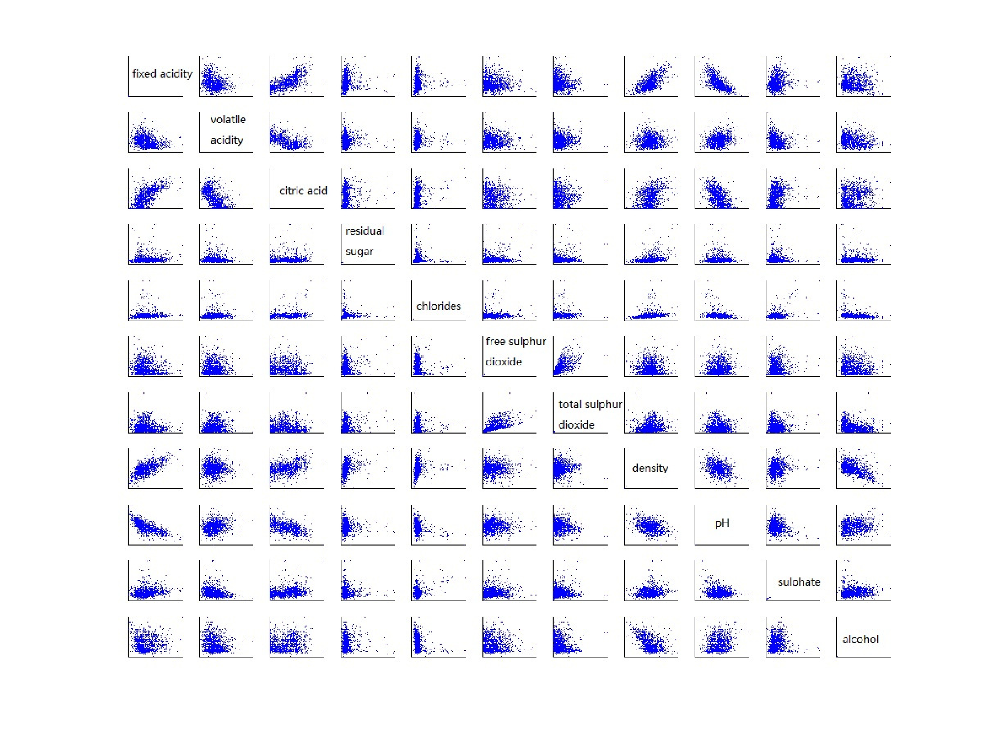
A matrix of scatterplots of $X_{j}$ against $X_{i}$ is shown in Figure 18, for $i=1,\ldots,11$ . These scatterplots visually indicate moderate correlations between the following pairs of variables: fixed acidity-citric acid, fixed acidity-density, fixed acidity-pH, volatile acidity-citric acid, free sulphur dioxide-total sulphur dioxide, density-alcohol. All these variables share an edge at probability $\geq 0.05$ in our learnt graphical model of data ${\bf D}_{S}^{(red)}$ (Figure 3 of main paper). We note that all moderately correlated variable pairs, as represented in these scatterplots, are joined by edges in our learnt graphical model of the red wine data–as is to be expected if the learning of the graphical model is correct. Such pairs include fixed acidity-citric acid, fixed acidity-density, fixed acidity-pH, volatile acidity-citric acid, free sulphur dioxide-total sulphur dioxide, density-alcohol. However, an edge may exist between a pair of variables even when the apparent empirical correlation between these variables is low (see Section 11); this owes to the effect of other variables. However, an edge may exist between a pair of variables even when the apparent empirical correlation between these variables is low (see Section 11), owing to the effect of other variables. Noticing such edges from the residual-sugar variable, we undertake a regression analysis (ordinary least squares) with residual-sugar regressed against the other remaining 10 vino-chemical variables. The MATLAB output of that analysis is included in Figure 19. The analysis indicates that the covariates with maximal (near-equal) effect on residual-sugar, are density and alcohol; residual-sugar is learnt to enjoy an edge with both density ( $Z_{7}$ ) and alcohol ( $Z_{10}$ ) in our learnt graphical model of the red wine data (Figure 3 of WC).

We also undertook a separate ordinary least squares analysis with the response variable quality, regressed against the vino-chemical variables as the covariates. The MATLAB output of this regression analysis in in Figure 20. We notice that the strongest (and nearly-equal) effect on quality is from the variables volatile-acidity and alcohol–the very two variables that share an edge at probability $\geq 0.05$ with quality, in our learnt graphical model of the red wine data.

14 Cholesky Factorisation and Matrix Inversion by Forward Substitution

Let a $p\times p$ -square positive-definite (correlation) matrix be $\boldsymbol{\Sigma}_{C}^{(S)}=\boldsymbol{L}_{C}^{(S)}(\boldsymbol{L}_{C}^{(S)})^{T}$ . The Cholesky factorisation of $\boldsymbol{\Sigma}_{C}^{(S)}=[s_{ij}]$ into its unique square root $\boldsymbol{L}_{C}^{(S)}=[l_{ij}]$ can be shown to be defined by the following scheme:

$\displaystyle l_{11}$	$\displaystyle=$	$\displaystyle\sqrt{s_{11}},$
$\displaystyle l_{i1}$	$\displaystyle=$	$\displaystyle\displaystyle{\frac{s_{i1}}{l_{11}}},\quad{i=1,\ldots,p},$
$\displaystyle l_{ij}$	$\displaystyle=$	$\displaystyle\displaystyle{\frac{\sqrt{s_{ij}-\sum\limits_{k=1}^{j-1}l_{ik}l_{kj}}}{l_{jj}}}\quad{j=1,\ldots,i-1;\>i=1,\ldots,p},$
$\displaystyle l_{ii}$	$\displaystyle=$	$\displaystyle\displaystyle{\sqrt{s_{ii}-\sum\limits_{k=1}^{i-1}l_{ik}^{2}}}\quad{i=2,\ldots,p},$

while forward substitution seeks $\boldsymbol{L}_{C}^{-1}$ s.t. $\boldsymbol{L}_{C}\boldsymbol{L}_{C}^{-1}=\boldsymbol{I}$ , where $\boldsymbol{I}$ is the $pXp$ -dimensional identity matrix. Then the scheme for forward substitution is the following:

$\displaystyle m_{11}$	$\displaystyle=$	$\displaystyle\displaystyle{\frac{1}{l_{11}}},$
$\displaystyle l_{i1}$	$\displaystyle=$	$\displaystyle\displaystyle{\frac{s_{i1}}{l_{11}}},\quad{i=1,\ldots,p},$
$\displaystyle l_{ij}$	$\displaystyle=$	$\displaystyle\displaystyle{\frac{\sqrt{s_{ij}-\sum\limits_{k=1}^{j-1}l_{ik}l_{kj}}}{l_{jj}}}\quad{j=1,\ldots,i-1;\>i=1,\ldots,p},$
$\displaystyle l_{ii}$	$\displaystyle=$	$\displaystyle\displaystyle{\sqrt{s_{ii}-\sum\limits_{k=1}^{i-1}l_{ik}^{2}}}\quad{i=2,\ldots,p},$

References

Airoldi (2007) [author] Airoldi, E. M.E. M. (2007). Getting Started in Probabilistic Graphical Models. PLoS Computational Biology 3 e252.
Bandyopadhyay and Canale (2016) [author] Bandyopadhyay, D.D. and Canale, A.A. (2016). Sparse Multi-Dimensional Graphical Models: A Unified Bayesian Framework. Journal of Rotyal Statistical society Series C 65 619-640.
Banerjee et al. (2015) [author] Banerjee, S.S., Basu, A.A., Bhattacharya, S.S., Bose, S.S., Chakrabarty, D.D. and Mukherjee, S.S. (2015). Minimum distance estimation of Milky Way model parameters and related inference. SIAM/ASA Journal on Uncertainty Quantification 3 91–115.
Benner et al. (2014) [author] Benner, P.P., Findeisen, R.R., Flockerzi, D.D., Reichl, U.U. and Sundmacher, K.K. (2014). Large-Scale Networks in Engineering and Life Sciences. Modeling and Simulation in Science, Engineering and Technology. Springer, Switzerland.
Bhattacharyya (1943) [author] Bhattacharyya, A.A. (1943). On a measure of divergence between two statistical populations defined by their probability distributions. Bull. Calcutta Math. Soc. 35 99–109.
Carvalho and West (2007) [author] Carvalho, C. M.C. M. and West, M.M. (2007). Dynamic matrix-variate graphical models. Bayesian Analysis 2 69–97. 10.1214/07-BA204
Cortez et al. (1998) [author] Cortez, P.P., Cerdeira, A.A., Almeida, F.F., Matos, T.T. and Reis, J.J. (1998). Modeling wine preferences by data mining from physicochemical properties. Decision Support Systems 47 547-553.
Dawid and Lauritzen (1993) [author] Dawid, A. P.A. P. and Lauritzen, S. L.S. L. (1993). Hyper-Markov laws in the statistical analysis of decomposable graphical models. Ann. Statist. 21 1272–1317.
Duff and Naylor (1966) [author] Duff, G. F. D.G. F. D. and Naylor, D.D. (1966). Differential equations of applied mathematics. John Wiley& Sons, Inc., New York-London-Sydney.
Frieze and Karonski (2016) [author] Frieze, A.A. and Karonski, M.M. (2016). Introduction to Random Graphs. Cambridge University Press, Cambridge.
Goodman (1970) [author] Goodman, L. A.L. A. (1970). The Multivariate Analysis of Qualitative Data: Interaction Among Multiple Classifications. Journal of the American Statistical Association 65 226-256.
Gruber and West (2016) [author] Gruber, L.L. and West, M.M. (2016). GPU-Accelerated Bayesian Learning and Forecasting in Simultaneous Graphical Dynamic Linear Models. Bayesian Analysis 11 125-149.
Guinness et al. (2014) [author] Guinness, J.J., Fuentes, M.M., Hesterberg, D.D. and Polizzotto, M.M. (2014). Multivariate spatial modeling of conditional dependence in microscale soil elemental composition data. Spatial Statistics 9 93-108.
Hajian-Tilaki (2013) [author] Hajian-Tilaki, K.K. (2013). Receiver Operating Characteristic (ROC) Curve Analysis for Medical Diagnostic Test Evaluation. Caspian Journal of Internal Medicine 4 627-635.
Hoehndorf, Schofield and Gkoutos (2015) [author] Hoehndorf, R.R., Schofield, P. N.P. N. and Gkoutos, G. V.G. V. (2015). Analysis of the human diseasome using phenotype similarity between common, genetic, and infectious diseases. Scientific Reports 5.
Hoff (2011) [author] Hoff, P. D.P. D. (2011). Separable covariance arrays via the Tucker product, with applications to multivariate relational data. Bayesian Analysis 6 179–196.
Kiiveri, Speed and Carlin (1984) [author] Kiiveri, H.H., Speed, T. P.T. P. and Carlin, J. B.J. B. (1984). Recursive Causal Models. Journal of the Australian Mathematical Society 36 30-52.
Lauritzen (1996) [author] Lauritzen, S. L.S. L. (1996). Graphical Models. Oxford University Press, Oxford, UK.
Madigan and Raftery (1994) [author] Madigan, D.D. and Raftery, A. E.A. E. (1994). Model Selection and Accounting for Model Uncertainty in Graphical Models Using Occam’s Window. Journal of the American Statistical Association 89 1535-1546.
Mathai and G.Pederzoli (1997) [author] Mathai, A. M.A. M. and Pederzoli, G.G. (1997). Some Properties of Matrix-Variate Laplace Transforms and Matrix-Variate Whittaker Functions 253. Elsevier Science, New York.
Matusita (1953) [author] Matusita, KameoK. (1953). On the estimation by the minimum distance method. Annals of the Institute of Statistical Mathematics 5 59–65.
Ni, Stingo and Baladandayuthapani (2017) [author] Ni, Y.Y., Stingo, F. C.F. C. and Baladandayuthapani, V.V. (2017). Sparse Multi-Dimensional Graphical Models: A Unified Bayesian Framework. Journal of the American Statistical Association 112 779-793.
Robert and Casella (2004) [author] Robert, C. P.C. P. and Casella, G.G. (2004). Monte Carlo Statistical Methods. Springer-Verlag, New York.
Wang and West (2009) [author] Wang, H.H. and West, M.M. (2009). Bayesian analysis of matrix normal graphical models. Biometrika 96 821–834.
Whittaker (2008) [author] Whittaker, J.J. (2008). Graphical Models in Applied Multivariate Statistics. Wiley, Switzerland.
Wothke (1993) [author] Wothke, W.W. (1993). Nonpositive definite matrices in structural modeling. Sage, Newbury Park, CA.
Xu, Yan and Qi. (2012) Xu, Z., Yan, F. and Qi., A. (2012). Infinite tucker decomposition: Nonparametric bayesian models for multiway data analysis. In Proceedings of the 29th International Conference on Machine Learning 1023–1030.
Liu (1988) [author] Liu, K.K. (1988). Measurement error and its impact on partial correlation and multiple linear regression analyses. Americal Jl.of Epidemiology 127 864–874.
Sheskin (2004) [author] Sheskin, D.D. (2004). Handbok of parametric and nonparametric statistical procedures. Chapman & Hall/CRC, Boca Raton, Florida.

$\displaystyle\left[\boldsymbol{\Sigma}_{C}^{(S)},\boldsymbol{\Sigma}_{R}^{(S)}\|{\bf D}_{S}\right]$	$\displaystyle\propto$	$\displaystyle\displaystyle{\ell\left(\boldsymbol{\Sigma}_{R}^{(S)},\boldsymbol{\Sigma}_{C}^{(S)}\|{\bf D}_{S}\right)\left[\boldsymbol{\Sigma}_{C}^{(S)},\boldsymbol{\Sigma}_{R}^{(S)}\right],\quad{\mbox{i.e.}}}$
$\displaystyle\left[\boldsymbol{\Sigma}_{C}^{(S)},\boldsymbol{\Sigma}_{R}^{(S)}\|{\bf D}_{S}\right]$	$\displaystyle\propto$	$\displaystyle\displaystyle{\frac{1}{(2\pi)^{\frac{np}{2}}{\Big\|}\boldsymbol{\Sigma}_{C}^{(S)}{\Big\|}^{\frac{p}{2}}{\Big\|}\boldsymbol{\Sigma}_{R}^{(S)}{\Big\|}^{\frac{n}{2}}}\times}$
		$\displaystyle\displaystyle{\exp\left[-\frac{1}{2}tr\left\{(\boldsymbol{\Sigma}_{R}^{(S)})^{-1}({\bf D}_{S})(\boldsymbol{\Sigma}_{C}^{(S)})^{-1}({\bf D}_{S})^{T}\right\}\right]{\Big\|\boldsymbol{\Sigma}_{R}^{(S)}\Big\|^{-\frac{n}{2}-1}}},$

	$\displaystyle D_{H}(p_{1},p_{2})\displaystyle{{\|\ell_{1}-\ell_{2}\|}}+D_{H}(p_{2},p_{3})\displaystyle{{\|\ell_{2}-\ell_{3}\|}}$	$\displaystyle<$	$\displaystyle D_{H}(p_{1},p_{3}){\|\ell_{1}-\ell_{3}\|}$
	$\displaystyle\leq D_{H}(p_{1},p_{2}){\|\ell_{1}-\ell_{3}\|}$	$\displaystyle+$	$\displaystyle D_{H}(p_{2},p_{3}){\|\ell_{1}-\ell_{3}\|}$

Correlation between Multivariate Datasets, from Inter-Graph Distance computed using Graphical Models Learnt With Uncertainties

Abstract

keywords

1 Introduction

2 Learning correlation matrix and graphical model given data, using Metropolis-within-Gibbs

Theorem 2.1.

Proof.

Proposition 2.1.

2.1 Learning the graphical model

2.2 Inference using Metropolis-within-Gibbs

2.3 Defining the 95%\% HPD credible regions on the random graph variable, and the learnt graphical model

Definition 2.1.

3 Uncertainties in learnt graphical models help compute inter-graph distance

Definition 3.1.

Remark 3.1.

Proposition 3.1.

3.1 Suggested inter-graph separation δ⁡(⋅,⋅)\delta(\cdot,\cdot), is an inter-graph distance

Theorem 3.1.

Proof.

Proposition 3.2.

4 Implementation on real data

4.1 Results given data 𝐃S(w​h​i​t​e){\bf D}^{(white)}_{S}

4.1.1 Comparing against earlier work done with white wine data

4.2 Results given data 𝐃S(r​e​d){\bf D}^{(red)}_{S}

4.2.1 Comparing against empirical work done with red wine data

5 Metric measuring distance between posterior probability densities of graphs given white and red wine datasets

6 Learning the human disease-symptom network

Definition 6.1.

6.1 Comparing our results to the earlier work done on the human disease-symptom network

7 Conclusion

Supplementary Material

8 Empirical illustration: simulated data

8.1 Learning correlation matrix &\& graph given toy data 𝐃T(S){\bf D}_{T}^{(S)}

8.2 Incorporating measurement uncertainties in the learnt graphical model

9 Model checking

10 Some results given the white wine data set

11 Comparing against previous work done with white wine data

12 Results of learning given the red wine data set

13 Comparing our learnt results against empirical and regression analysis of red-wine data

14 Cholesky Factorisation and Matrix Inversion by Forward Substitution

References

2.3 Defining the 95 $\%$ HPD credible regions on the random graph variable, and the learnt graphical model

3.1 Suggested inter-graph separation $\delta(\cdot,\cdot)$ , is an inter-graph distance

4.1 Results given data ${\bf D}^{(white)}_{S}$

4.2 Results given data ${\bf D}^{(red)}_{S}$

8.1 Learning correlation matrix $\&$ graph given toy data ${\bf D}_{T}^{(S)}$