Synchronization in Networks of Diffusively Coupled Nonlinear Systems:
Robustness Against Time-Delays

The emergence of synchronization in networks of coupled dynamical systems is a fascinating topic in various scientific disciplines ranging from biology, physics, and chemistry to social networks and technological applications. For instance, in biology, it is well known that thousands of fireflies light up simultaneously [30], and that groups of Japanese tree frogs (Hyla japonica) may show synchronous behavior in their calls [1]. In medicine and neuroscience, clusters of synchronized pacemaker neurons regulate our heartbeat [21], synchronized neurons in the olfactory bulb allow us to detect and distinguish between odors [8], and our circadian rhythm is synchronized to the 24-h day-night cycle [4]. In engineering, elements of synchronization are present in power networks [6], in the velocity of platoons of vehicles [23], and in robotics, where multiple robots carry out tasks that cannot be achieved by a single one [17]. Several more examples of synchronous behavior in science and engineering can be found in, for instance, (Refs. [2, 22, 30, 12, 11, 29]) and references therein.

One of the first technical results regarding synchronization of coupled nonlinear systems is presented in (Refs. [7, 20]). In these papers, the authors show that coupled chaotic oscillators may synchronize in spite of their high sensitivity to initial conditions. After these results, considerable interest in the notion of synchronization of general nonlinear systems has arisen. Here, we focus on synchronization in networks of identical nonlinear systems interacting through diffusive time-delayed couplings on networks with general topologies. Diffusive time-delayed couplings arise naturally for interconnected systems since the transmission of signals is expected to take some time. Time-delays caused by signal transmission and/or faults in the communication channels affect the behavior of the interconnected systems (e.g., in terms of stability and/or performance).

This manuscript follows the same research line as (Refs. [24, 26, 28, 13, 14]), where sufficient conditions for synchronization of diffusively time-delayed coupled semipassive systems with and without time-delays are presented. In particular, the authors in Ref. [26] prove that under some mild conditions, there always exists a region $\mathcal{S}$ in the parameter space (coupling strength $\gamma$ versus time-delay $\tau$), such that if $(\gamma,\tau)\in\mathcal{S}$ then the systems synchronize. In order to derive their results, the authors assume that the individual systems are semipassive [25] with respect to the coupling variable (the measurable output) and the corresponding internal dynamics has some desired stability properties (convergent internal dynamics [19]). In the same spirit, here we prove that the region $\mathcal{S}$ is always bounded by a unimodal function $\varphi(\gamma)$ defined on some set $\mathcal{J}\subset{\mathds{R}}$; and consequently, that there always exists an optimal coupling strength $\gamma^{*}$ that leads to the maximum time-delay $\tau^{*}=\varphi(\gamma^{*})$ that can be induced to the network without compromising the synchronous behavior. Therefore, for $\gamma=\gamma^{*}$ and for any $\tau\leq\tau^{*}$, the systems synchronize, i.e., the gain $\gamma=\gamma^{*}$ leads to the best tolerance against time-delays of the closed-loop dynamics. Moreover, we analyze the effect of the network topology on the values of both the optimal $\gamma^{*}$ and the maximum time-delay $\tau^{*}$, i.e., we show how the eigenvalues of the corresponding Laplacian matrix affect $\varphi(\gamma)$, $\gamma^{*}$, and $\tau^{*}$. This, in turn, gives insights into designing the network topology in order to enhance robustness against time-delays. The results of this manuscript are based on our preliminary conference paper Ref. [15].

The remainder of the paper is organized as follows. In Section 2, we recall some important definitions needed for the subsequent sections. The notion of semipassivity, convergent systems, and some basic terminology of graph theory are introduced. The class of systems under study, the definition of diffusive time-delayed couplings, and the problem formulation are given in Section 3. The main results are presented in Section 4. Simulation experiments of coupled Hindmarsh-Rose neurons are given in Section 5 to illustrate our results. Finally, concluding remarks are presented in Section 6.

Throughout this paper, the following notation is used: the symbol ${\mathds{R}}_{>0}$(${\mathds{R}}_{\geq 0}$) denotes the set of positive (nonnegative) real numbers. The Euclidian norm in ${\mathds{R}}^{n}$ is denoted simply as $|\cdot|$, $|x|^{2}=x^{T}x$, where ^T defines transposition. The notation $\text{col}(x_{1},...,x_{n})$ stands for the column vector composed of the elements $x_{1},...,x_{n}$. This notation will be also used in case the components $x_{i}$ are vectors. The induced norm of a matrix $A\in{\mathds{R}}^{n\times n}$, denoted by $\|A\|$, is defined as $\|A\|=\max_{x\in{\mathds{R}}^{n},|x|=1}|Ax|$. The $n\times n$ identity matrix is denoted by $I_{n}$ or simply $I$ if no confusion can arise. Likewise, the $n\times m$ matrices composed of only ones and only zeros are denoted as $\mathbf{1}_{n\times m}$ and $\mathbf{0}_{n\times m}$, respectively. The spectrum of a matrix $A$ is denoted by $spec(A)$. For any two matrices $A$ and $B$, the notation $A\otimes B$ (the Kronecker product [3]) stands for the matrix composed of submatrices $A_{ij}B$ , where $A_{ij}$, $i,j=1,...,n$, stands for the $ij$th entry of the $n\times n$ matrix $A$. Let $\mathcal{X}\subset{\mathds{R}}^{n}$ and $\mathcal{Y}\subset{\mathds{R}}^{m}$. The space of continuous functions from $\mathcal{X}$ to $\mathcal{Y}$ is denoted by $\mathcal{C}(\mathcal{X},\mathcal{Y})$. If the functions are (at least) $r\geq 0$ times continuously differentiable, then it is denoted by $\mathcal{C}^{r}(\mathcal{X},\mathcal{Y})$. If the derivatives of a function of all orders ($r=\infty$) exist, the function is called smooth and if the derivatives up to a sufficiently high order exist the function is named sufficiently smooth. For simplicity of notation, we often omit the explicit dependence of time $t$.

Consider $k$ identical nonlinear systems of the form

with $i\in\mathcal{I}:=\{1,...,k\}$, state $x_{i}:=\text{col}(\zeta_{i},y_{i})\in{\mathds{R}}^{n}$, internal state $\zeta_{i}\in{\mathds{R}}^{n-m}$, output $y_{i}\in{\mathds{R}}^{m}$, input $u_{i}\in{\mathds{R}}^{m}$, sufficiently smooth functions $q:{\mathds{R}}^{n-m}\times{\mathds{R}}^{m}\rightarrow{\mathds{R}}^{n-m}$ and $a:{\mathds{R}}^{n-m}\times{\mathds{R}}^{m}\rightarrow{\mathds{R}}^{m}$, matrices $C\in{\mathds{R}}^{m\times n}$ and $B\in{\mathds{R}}^{n\times m}$, and the matrix $CB\in{\mathds{R}}^{m\times m}$ being similar to a positive definite matrix. For the sake of simplicity, it is assumed that $CB=I_{m}$ (results for the general case with $CB$ being similar to a positive definite matrix can be easily derived). It is assumed that (3)-(4) is strictly $\mathcal{C}^{1}$-semipassive and the internal dynamics [18] (3) is an exponentially convergent system. Let the $k$ systems (3)-(4) interact on simple strongly connected graph through the diffusive time-delayed coupling

where $\tau\in{\mathds{R}}_{\geq 0}$ denotes a constant time-delay, $y_{j}(t-\tau)$ and $y_{i}(t-\tau)$ are the time-delayed outputs of the $j$-th and $i$-th systems, $\gamma\in{\mathds{R}}_{\geq 0}$ denotes the coupling strength, $a_{ij}\geq 0$ are the weights of the interconnections, and $\mathcal{E}_{i}$ is the set of neighbors of system $i$. It is assumed that the graph is undirected, i.e., $a_{ij}=a_{ji}$. Moreover, since the coupling strength is encompassed in the constant $\gamma$, it is assumed without loss of generality that $\text{max}_{i\in\mathcal{I}}\sum_{j\in\mathcal{E}_{i}}a_{ij}=1$. Note that all signals in coupling (5) are time-delayed. Such a coupling may arise, for instance, when the systems are interconnected through a centralized control law. Coupling (5) can be written in matrix form as follows

with $u:=\text{col}(u_{1},\ldots,u_{k})$, $y:=\text{col}(y_{1},\ldots,y_{k})$, and Laplacian matrix $L=L^{T}\in{\mathds{R}}^{k\times k}$. The authors in Ref. [26] prove that the $k$ coupled systems (3)-(5) asymptotically synchronize provided that $\gamma$ is sufficiently large and the product of the coupling strength and the time-delay $\gamma\tau$ is sufficiently small. It follows that there exists a region $\mathcal{S}$ in the parameter space, such that if $(\gamma,\tau)\in\mathcal{S}$, the systems synchronize. In this manuscript, we go one step further by showing that this region $\mathcal{S}$ is actually bounded by a unimodal function $\varphi:\mathcal{J}\to{\mathds{R}}_{\geq 0}$, $\gamma\mapsto\varphi(\gamma)$. Therefore, there exists an optimal coupling strength $\gamma^{*}$ that leads to the maximum delay $\tau^{*}=\varphi(\gamma^{*})$ that can be induced without compromising the synchronous behavior. Moreover, we characterize the function $\varphi(\gamma)$, the optimal $\gamma^{*}$, and the maximum time-delay $\tau^{*}$ in terms of the spectrum of the Laplacian matrix $L$ and the vector fields $q(\cdot)$ and $a(\cdot)$.

In this section, we give sufficient conditions for synchronization in networks of the diffusively time-delayed coupled semipassive systems. However, before we start thinking about synchronization, it is necessary to ensure that the solutions of the closed-loop system (3)-(5) are well defined, i.e., the solutions exist and are bounded. In the following lemma (adapted from Ref. [26]), we give sufficient conditions for ultimate boundedness [10] of the solutions of the coupled systems interacting on simple strongly connected graphs.

Proof: By assumption, each system (3)-(4) is strictly $\mathcal{C}^{1}$-semipassive with input $u_{i}$, output $y_{i}$, and radially unbounded function $V(x_{i})$. Define the functional

where $x=\text{col}(x_{1},...,x_{k})$, $x_{t}(\theta)=x(t+\theta)\in\mathcal{C}$, $\theta\in[-\tau,0]$, $\mathcal{C}=[-\tau,0]\rightarrow{\mathds{R}}^{kn}$ being the Banach space of continuous functions mapping the interval $[-\tau,0]$ into ${\mathds{R}}^{kn}$, and the constants $\nu_{i}$ denoting the entries of the left eigenvector corresponding to the simple zero eigenvalue of the Laplacian matrix $L$, i.e., $\nu=\left(\nu_{1},...,\nu_{k}\right)^{T}$ and $\nu^{T}L=\nu^{T}\left(D-A\right)=0$. Note that $L$ is singular by construction and since it is assumed that the graph is strongly connected, then the zero eigenvalue is simple. Using the Perron-Frobenius theorem, it can be shown that the vector $\nu$ has strictly positive real entries, i.e., $\nu_{i}>0$ for all $i\in\mathcal{I}$, see Ref. [3]. Then, by assumption

Consider the term

using Young’s inequality, it follows that

Combining the previous results and using the fact that $\nu^{T}L=0$, and $\max_{i\in\mathcal{I}}\sum_{j\in\mathcal{E}_{i}}a_{ij}=1$, the following is satisfied $\dot{W}\leq\sum_{i=1}^{k}\nu_{i}(-H(x_{i})+2\gamma\left|y_{i}\right|^{2})$. By assumption (H4.1), there exist positive constants $R,\delta\in{\mathds{R}}_{>0}$ such that $|x_{i}|>R$ implies that $H(x_{i})-\delta|y_{i}|^{2}>0$. Let $\bar{\delta}$ be the largest $\delta$ that satisfies (H4.1) for arbitrarily large $R<\infty$. Then, for $\gamma$ satisfying $2\gamma\leq\bar{\delta}$ and for sufficiently large $|x|$, it follows that $\dot{W}<0$. By construction, the functional $W$ is lower and upper bounded by some $\mathcal{K}_{\infty}$-functions [10]. Hence, there exists a constant $\sigma\in{\mathds{R}}_{>0}$ such that $\dot{W}<0$ for $\sigma$ and $x$ satisfying ${W}(x)\geq\sigma$. Then, solutions starting in the set $\{W(x)\leq\sigma\}$ will remain there for future time since $\dot{W}$ is negative on the boundary $W(x)=\sigma$. Moreover, for any $x$ in the set $\{W(x)\geq\sigma^{*}\}$ with $\sigma^{*}>\sigma$, the function $\dot{W}(x)$ is strictly negative, which implies that, in this set, $W(x)$ decreases monotonically until the solutions enter the set $\{W(x)\leq\sigma\}$ again; and therefore, we can conclude that the solutions of the closed-loop system (3)-(5) exist and are ultimately bounded for any finite $\tau\geq 0$ and $\gamma\leq\frac{\bar{\delta}}{2}$. $\blacksquare$

Next, we give sufficient conditions for global synchronization of the coupled systems. Define the stacked state $x:=\text{col}(x_{1},\ldots,x_{k})$ ($x_{i}:=\text{col}(\zeta_{i},y_{i})$) and the synchronization manifold $\mathcal{M}:=\{x\in{\mathds{R}}^{kn}\text{ }|\hskip 1.42262ptx_{i}=x_{j},\hskip 1.42262pt\forall\text{ \ }i,j\in\mathcal{I}\}$. The coupled systems (3)-(5) are said to synchronize if the synchronization manifold $\mathcal{M}$ is invariant under the closed-loop dynamics and contains an asymptotically stable subset. Clearly, if the systems are interconnected through (5), the coupling functions vanish on $\mathcal{M}$; hence, the manifold $\mathcal{M}$ is positively invariant under the dynamics (3)-(5), see Ref. [28] for details. In the following theorem, we give conditions for the existence of an asymptotically stable subset of the synchronization manifold. In particular, we prove that under some mild assumptions, there exists a region $\mathcal{S}$ bounded by a unimodal function such that if $(\gamma,\tau)\in\mathcal{S}$, the systems synchronize.

The proof of Theorem 1 can be found in the appendix. The result stated in Theorem 1 amounts to the following. The solutions of (3)-(5) are ultimately bounded and the systems asymptotically synchronize provided that the coupling strength $\gamma$ is sufficiently large and the time-delay $\tau$ is smaller than some unimodal function $\varphi(\gamma)$, see Figure 1. Therefore, there exists a region $\mathcal{S}$ (colored area in Figure 1) such that if $(\gamma,\tau)\in\mathcal{S}$, there exists a globally asymptotically stable subset of the synchronization manifold $\mathcal{M}$. Estimates of both the constant $\gamma^{\prime}$ and the unimodal function $\varphi(\gamma)$ are derived in the proof of Theorem 1, in (30) and (A.1), respectively. They depend on the network topology (more specifically on the eigenvalues of the Laplacian matrix), the dynamics of the individual subsystems, i.e., the vector fields $q(\cdot)$ and $a(\cdot)$, and the bounds on the solutions of the closed-loop system. Note that our results are meant to prove existence of the synchronization region $\mathcal{S}$ and to provide a qualitative analysis of the unimodal bound $\varphi(\gamma)$; the estimates of $\gamma^{\prime}$ and $\varphi(\gamma)$ given in appendix may be conservative.

The result stated in Corollary 1 implies that for every strongly connected graph $\mathcal{G}$, there exists an optimal coupling strength $\gamma^{*}$ that leads to the maximum time-delay $\tau^{*}=\varphi(\gamma^{*})=\max(\tau\in\mathcal{S})$ that can be induced to the network without compromising the synchronous behavior, i.e., there exists a gain $\gamma=\gamma^{*}$ that leads to the best tolerance against time-delays of the closed-loop system, see Figure 1. In the following corollary, we characterize the effect of the network topology on the values of both the optimal $\gamma^{*}$ and the maximum time-delay $\tau^{*}$, i.e., we study the effect of the eigenvalues of the Laplacian matrix $L$ on the unimodal function $\varphi(\gamma)$.

Let $\bar{\mathcal{G}}:=\{\mathcal{G}_{s}\hskip 2.84526pt|\hskip 2.84526pts\in\mathbb{N}\hskip 2.84526pt\}$ denote the set of all simple strongly connected undirected graphs. For each graph $\mathcal{G}_{s}$, consider $k=k_{s}$ coupled systems (3)-(5) with coupling strength $\gamma=\gamma_{s}\in{\mathds{R}}_{\geq 0}$ and delay $\tau=\tau_{s}\in{\mathds{R}}_{\geq 0}$ interacting on $\mathcal{G}_{s}$. Assume that the conditions stated in Theorem 1 are satisfied, then from Theorem 1, there exist constants $\gamma_{s}^{\prime}\in{\mathds{R}}_{>0}$ and unimodal functions $\varphi_{s}:\mathcal{J}_{s}\rightarrow{\mathds{R}}_{\geq 0}$, $s\in\mathbb{N}$, such that if $(\gamma_{s},\tau_{s})\in\mathcal{S}_{s}$, where

the $k_{s}$ systems of each $\mathcal{G}_{s}$ asymptotically synchronize. Let $\gamma_{s}^{*}$ and $\tau_{s}^{*}=\max(\tau_{s}\in\mathcal{S}_{s})$ be the optimal coupling strength and the corresponding maximum time-delay of $\mathcal{G}_{s}$ and define $\bar{\tau}^{*}:=\{\tau_{s}^{*}\hskip 2.84526pt|\hskip 2.84526pts\in\mathbb{N}\hskip 2.84526pt\}$, i.e., the set of all maximum time-delays of $\bar{\mathcal{G}}$, and

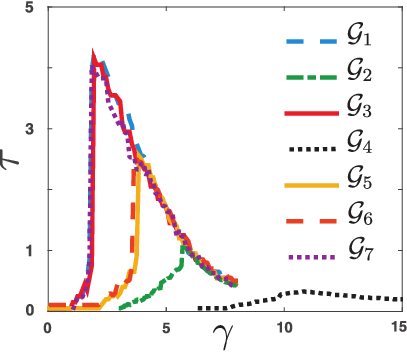
The proof of Corollary 2 can be found in the appendix. The result stated in Corollary 2 amounts to the following. The effect of the network topology on the maximum time-delay $\tau^{*}$ is solely determined by the quotient $(\frac{\lambda_{k}}{\lambda_{2}})$. Case (a): implies that any two strongly connected networks with the same quotient $(\lambda_{k}/\lambda_{2})$ have the same maximum time-delay $\tau^{*}$. Additionally, in this case, the value of the optimal coupling strength $\gamma^{*}$ is also determined by $\lambda_{2}$, i.e., if the two networks have the same quotient, then the larger the $\lambda_{2}$ the smaller the $\gamma^{*}$, and vice versa. Case (b): implies that networks with quotient equal to one have the best tolerance against time-delays, i.e., if $\frac{\lambda_{k}}{\lambda_{2}}=1$, then $\tau^{*}=\tau^{*}_{\max}$ with $\tau^{*}_{\max}$ as defined in (9). Finally, case (c) implies that the larger the quotient $\frac{\lambda_{k}}{\lambda_{2}}$ the smaller the $\tau^{*}$, and vice versa. See Figure 2.

A. Network Topology, Strict Semipassivity, and Convergence. Consider a network of $k_{s}$, $s\in\{1,\ldots,7\}$, systems coupled according to the graphs $\mathcal{G}_{s}$ depicted in Figure 3. For each network, the weights of the interconnections are set to $a_{ij}=1/k_{s}$ if $\{i,j\}\in\mathcal{E}_{s}$ and $a_{ij}=0$ otherwise. The networks are strongly connected and undirected. Each system in the networks is assumed to be a Hindmarsh-Rose neuron[9], of the form

with output $y_{i}\in{\mathds{R}}$, internal states $\zeta_{i1},\zeta_{i2}\in{\mathds{R}}$, state $x_{i}=\text{col}(\zeta_{i1},\zeta_{i2},y_{i})\in{\mathds{R}}^{3}$, input $u_{i}\in{\mathds{R}}$, and $i\in\mathcal{I}=\{1,\ldots,k_{s}\}$. It is well known that the Hindmarsh-Rose neuron (10) has a chaotic attractor for $u_{i}=0$, see Ref. [9]. Furthermore, in Ref. [27], the authors prove that the Hindmarsh-Rose neuron is strictly $\mathcal{C}^{1}$-semipassive with storage function $V(\zeta_{1i},\zeta_{2i},y_{i}):=\frac{1}{2}y_{i}^{2}+\sigma\zeta_{1i}^{2}+25\zeta_{2i}^{2}$, constants $\varsigma_{1},\varsigma_{2}\in(0,1)$, $0<\sigma<\frac{4\varsigma_{1}(1-\varsigma_{2})}{25}$, and

Moreover, the ($\zeta_{1i},\zeta_{2i}$)-dynamics (the internal dynamics) is exponentially convergent (in the sense of Definition 2), i.e., it satisfies the Demidovich condition (8) with $P=I_{2}$; hence, assumption (H4.2) in Theorem 1 is satisfied. This particular experiment is taken from Ref. [16], where a detailed experimental study is presented.
B. Bounded Solutions and Synchronization. It can be easily verified that the function $H(x_{i})$ in (11) satisfies the boundedness assumption (H4.1) for arbitrary large coupling strength $\gamma$. Therefore, by Lemma 1, the solutions of the coupled systems (10),(5) with $\gamma=\gamma_{s}$ and $\tau=\tau_{s}$ are ultimately bounded for any finite coupling strength $\gamma_{s}$ and time-delay $\tau_{s}$. Finally, given that all the graphs in Figure 3 are strongly connected and (H4.1) and (H4.2) are satisfied, then, by Theorem 1, there exist regions $\mathcal{S}_{s}$, $s=1,\ldots,7$, (as depicted in Figure 1), such that if $(\gamma_{s},\tau_{s})\in\mathcal{S}_{s}$, the systems synchronize.
C. Simulation Results. In Figure 4, we show results obtained through extensive computer simulations. We depict the synchronization regions $\mathcal{S}_{s}$, $s=1,\ldots,7$ for each network topology $\mathcal{G}_{s}$. These regions are clearly bounded by unimodal functions; and therefore, for each network, there exists an optimal coupling strength $\gamma^{*}_{s}$ and its corresponding maximum time-delay $\tau^{*}_{s}$ that can be induced to the network without compromising the synchronous behavior. These maximum time-delays are strongly influenced by the network topology, (see the proofs of Theorem 1 and Corollary 2). In Table 1, we show the numerical values of the optimal coupling strengths, the maximum time-delays, and the quotients $\lambda_{k_{s}}/\lambda_{2}$. These values match with the theoretical predictions given in Corollary 2.

We have presented a result on network synchronization of coupled nonlinear systems in the case when the coupling functions are subject to constant time-delays. Using the notions of semipassivity and convergent systems, we have provided sufficient conditions which guarantee ultimate boundedness of the solutions of the coupled systems and (global) state synchronization. In particular, we have proved that, under some mild assumptions, there always exists a region $\mathcal{S}$ in the parameter space (coupling strength $\gamma$ versus time-delay $\tau$), such that if $\gamma,\tau\in\mathcal{S}$, the systems synchronize. We proved that this region $\mathcal{S}$ is always bounded by a unimodal function $\varphi(\gamma)$; and consequently, that there always exists an optimal coupling strength $\gamma^{*}$ which leads to the maximum time-delay $\tau^{*}=\varphi(\gamma^{*})$ that the network can tolerate without breaking the synchrony. In Corollary 2, we have provided tools for selecting the network topology in order to enhance robustness against time-delays of the coupled systems. Case (b) in Corollary 2 implies that networks with quotient $(\lambda_{k}/\lambda_{2})$ equal to 1 have the best tolerance against time-delays. This is the case for all-to-all networks. Finally, we have presented a simulation example using networks of Hindmarsh-Rose neurons to illustrate the results.

References

- [1] I. Aihara, R. Takeda, T. Mizumoto, T. Otsuka, T. Takahashi, and H. Okuno. Complex and transitive synchronization in a frustrated system of calling frogs. Phys. Rev. E, 83:031913, 2011.
- [2] I. Blekhman. Synchronization in science and technology. ASME, New York, 1988.
- [3] B. Bollobas. Modern Graph Theory. Springer-Verlag, New York, 1998.
- [4] CA Czeisler, E Weitzman, MC Moore-Ede, JC Zimmerman, and RS Knauer. Human sleep: its duration and organization depend on its circadian phase. Science, 210:1264–1267, 1980.
- [5] B.P. Demidovich. Lectures on Stability Theory. Moscow. In Russian, 1967.
- [6] F. Dorfler and F. Bullo. Synchronization and transient stability in power networks and non-uniform kuramoto oscillators. SIAM Journal on Control and Optimization, 50(3):1616–1642, 2012.
- [7] H. Fujisaka and T. Yamada. Stability theory of synchronized motion in coupled-oscillator systems. Progress of Theoretical Physics, 69:32–37, 1983.
- [8] C. Gray. Synchronous oscillations in neuronal systems: Mechanisms and functions. Journal of Computational Neuroscience, 1:11–38, 1994.
- [9] J. L. Hindmarsh and R. M. Rose. A model of neuronal bursting using three coupled first order differential equations. Proceedings of the Royal Society of London B: Biological Sciences, 221:87–102, 1984.
- [10] H. K. Khalil. Nonlinear Systems. Prentice-Hall, 3nd edition, 2002.
- [11] C. Murguia, R. H. B. Fey, and H. Nijmeijer. Network synchronization by dynamic diffusive coupling. International Journal of Bifurcation and Chaos, 23:1350076, 2013.
- [12] C. Murguia, R. H. B. Fey, and H. Nijmeijer. Synchronization of identical linear systems and diffusive time-delayed couplings. IEEE Transactions on Circuits and Systems I: Regular Papers, 61:1801–1814, 2014.
- [13] C. Murguia, Rob H. B. Fey, and H. Nijmeijer. Network synchronization of time-delayed coupled nonlinear systems using predictor-based diffusive dynamic couplings. Chaos, 25:023108, 2015.
- [14] C. Murguia, Rob H. B. Fey, and H. Nijmeijer. Network synchronization using invariant-manifold-based diffusive dynamic couplings with time-delay. Automatica, 57:34 – 44, 2015.
- [15] C. Murguia, J. Ruths, and H. Nijmeijer. Robust network synchronization of time-delayed coupled systems. IFAC-PapersOnLine, 49:74 – 79, 2016.
- [16] P. Neefs, E. Steur, and H. Nijmeijer. Network complexity and synchronous behavior an experimental approach. Int. J. of Neural Systems, 20:233–247, 2010.
- [17] H. Nijmeijer and A. Rodriguez-Angeles. Synchronization of Mechanical Systems. World Scientific, 2003.
- [18] H. Nijmeijer and A. van der Schaft. Nonlinear dynamical control systems. Springer, New York, 1990.
- [19] A. Pavlov, A. Pogromsky, N. van de Wouw, and H. Nijmeijer. Convergent dynamics, a tribute to Boris Pavlovich Demidovich. Syst. Control Lett., 52:257, 2004.
- [20] L. M. Pecora and T. L. Carroll. Synchronization in chaotic systems. Phys. Rev. Lett., 64:821–824, 1990.
- [21] C.S. Peskin. Mathematical aspects of heart physiology. Courant Institute of Mathematical Sciences, New York University, 1975.
- [22] A. Pikovsky, M. Rosenblum, and J. Kurths. Synchronization: A universal concept in nonlinear Science. Cambridge University Press, Cambridge, 2001.
- [23] J. Ploeg, D.P. Shukla, N. van de Wouw, and H. Nijmeijer. Controller synthesis for string stability of vehicle platoons. Intelligent Transportation Systems, IEEE Transactions on, 15:854–865, 2014.
- [24] A. Pogromsky. Passivity based design of synchronizing systems. International Journal of Bifurcation and Chaos, 8:295–319, 1998.
- [25] A. Pogromsky, T. Glad, and H. Nijmeijer. On diffusion driven oscillations in coupled dynamical systems. Int. J. Bif. Chaos, 9:629–644, 1999.
- [26] E. Steur and H. Nijmeijer. Synchronization in networks of diffusively time-delay coupled (semi-)passive systems. IEEE Transactions on Circuits and Systems-I, 58(6):1358–1371, 2010.
- [27] E. Steur, I. Tyukin, and H. Nijmeijer. Semi-passivity and synchronization of diffusively coupled neuronal oscillators. Physica D, 238:2119–2128, 2009.
- [28] Erik Steur, Wim Michiels, Henri Huijberts, and Henk Nijmeijer. Networks of diffusively time-delay coupled systems: Conditions for synchronization and its relation to the network topology. Physica D: Nonlinear Phenomena, 277:22 – 39, 2014.
- [29] Erik Steur, Carlos Murguia, Rob H. B. Fey, and Henk Nijmeijer. Synchronization and partial synchronization experiments with networks of time-delay coupled hindmarshrose neurons. International Journal of Bifurcation and Chaos, 26:1650111, 2016.
- [30] S. Strogatz. SYNC. The emerging science of spontaneous Order. Hyperion, New York, 2003.
- [31] Jan C. Willems. Dissipative dynamical systems part i: General theory. Archive for Rational Mechanics and Analysis, 45:321–351, 1972.