An Integrated Approach to Crowd Video Analysis: From Tracking to Multi-level Activity Recognition

Neha Bhargava Affiliation: Indian Institute of Technology Bombay Affiliation: India Email: neha@ee.iitb.ac.in Subhasis Chaudhuri Affiliation: Indian Institute of Technology Bombay Affiliation: India Email: sc@ee.iitb.ac.in

Abstract

We present an integrated framework for simultaneous tracking, group detection and multi-level activity recognition in crowd videos. Instead of solving these problems independently and sequentially, we solve them together in a unified framework to utilize the strong correlation that exists among individual motion, groups and activities. We explore the hierarchical structure hidden in the video that connects individuals over time to produce tracks, connects individuals to form groups and also connects groups together to form a crowd. We show that estimation of this hidden structure corresponds to track association and group detection. We estimate this hidden structure under a linear programming formulation. The obtained graphical representation is further explored to recognize the node values that corresponds to multi-level activity recognition. This problem is solved under a structured SVM framework. The results on publicly available dataset show very competitive performance at all levels of granularity with the state-of-the-art batch processing methods despite the proposed technique being an online (causal) one.

1 Introduction

A crowd video analysis system first detects the individuals and then tracks them over time. These tracks are used for higher level applications such as group detection and activity recognition. This approach is sequential in nature whereas the various components of the system are highly correlated and influence each other. For example, a particular group activity motivates its group member for a particular action and all the groups together define the crowd activity. On the other hand, group behavior is influenced by its members and the overall crowd behavior. Effectively, these components - individual’s motion, groups, group activity and collective activity are correlated and can be expressed in a hierarchical structure. Hence it is more appropriate to estimate them together instead of sequentially. See Figure 1 as an example of this hierarchical structure where the atomic actions of the individuals are all standing, there are two groups each with group activity as talking and thus leading to the collective activity also as talking. These inherent dependencies among the various components motivate us to explore this idea of simultaneous recognition of tracks, groups and activities. We propose a novel approach to build on the detections to obtain the tracks, groups and activities in a causal framework, i.e. without considering future frames into estimation process. We solve this unified problem in two passes. The first pass consists of finding the graph structure that corresponds to the track association and group detection. We propose an linear programming based formulation for the same. The second pass involves activity recognition at various levels of granularity. We formulate this problem under the structured SVM formulation [29].

In this paper, the term action refers to an atomic movement performed by a single person, the term group activity denotes an activity performed by a group and collective activity refers to the activity performed by all the groups collectively. The paper is organized as follows. The next section discusses the related work followed by our contributions. The proposed model is described in Section 3. The subsequent Sections 4, 5 and 6 elaborate on frameworks for multi-target tracking with group detection followed by activity recognition. Experimentation details are provided in Section 7 and the paper concludes in Section 8.

2 Related work

The task of multi-target tracking (MTT) is to correctly associate all the detections (or tracklets) corresponding to each individual. Linear programming (LP) based global optimization for MTT is a popular approach. Many approaches formulate MTT either as min-cost flow optimization problem or MAP and use LP to find the global optimum. [9, 6, 35, 20, 4]. Recently, the approaches of utilizing social behavior to improve tracking are gaining attention [15, 5, 22, 19, 34]. The idea is to simultaneously associate a detection to a track and to a group. Our approach for obtaining groups is similar to that of [22] where they combine track association with grouping under a LP framework. Since the number of groups $K$ is unknown, they run the algorithm with all possible values of $K$ with a linear penalty. Our proposed method exploits the group information from the previous time instant and does not require to run for all values of $K$ resulting in a fast convergence.

Due to its various applications in video surveillance, activity recognition has been an active area of research. The survey on action and activity recognition can be found in [30, 32, 21]. There are many works dealing with single person action [12, 18, 17, 26, 31] and with single group activity recognition [8, 16, 24, 11, 25]. Recently, researchers have started exploring the problem of joint recognition of these actions and activities under a hierarchical framework [13, 14, 7, 3, 2]. Amer et al. in [2] proposed a hierarchical random field based modeling of higher order temporal dependencies of video features. Lan et al. in [14] jointly estimate actions, pairwise interactions and group activity. However, they assume the availability of action labels and they do not handle track association. Choi and Savarese in [7] proposed a hierarchical model and combine the problems of tracklet association and multi-level activity recognition (action, pairwise interaction and collective). All these methods either assumed availability of action label or trackelets whereas our proposed framework requires only detections.

Our work in this paper advances the existing approaches and add one more intermediate layer (i.e. grouping layer) in the hierarchy as shown in Figure 2a and explained in Section 3. The main contributions of this work are as follows:

1.

We propose a hierarchical graphical structure that combines multi-target tracking, group detection and activity recognition under an unified framework.
2.

We built a causal framework that takes only human detections as an input and outputs tracks, groups and activities at each time step.
3.

We propose an iterative linear programming based method for simultaneous track association and group detection.
4.

We propose an approach for simultaneous recognition of activities at various levels of granularity under a structured SVM framework.
5.

To make it suitable for real-time applications, we provide a fast algorithm for both training and inferencing.

3 The Proposed Model

In this section, we discuss the proposed model. Let $y_{k}\in\mathcal{Y}$ be the collective activity at time $k$ with group activity vector $\mathbf{g}_{k}=[g_{1k},g_{2k},...,g_{mk}]$ where $g_{ik}\in\mathcal{G}$ is the activity of $i^{th}$ group and $m$ be the number of groups present at time instant $k$ . The atomic activity vector is denoted as $\mathbf{h}_{k}=[h_{1k},h_{2k},...,h_{kN}]$ with $h_{ik}\in\mathcal{H}$ as the atomic activity of the $i^{th}$ person and $N$ is the total number of persons present at time $k$ . Let $\mathbf{T}_{k-1}$ denotes the estimated tracks available till time $k-1$ and $\mathbf{G}_{k}$ be the group label vector of length $N$ where its $i^{th}$ entry denotes the group label for the $i^{th}$ detection at time $k$ . Let $\mathbf{d}_{k}$ denotes the detections at time $k$ . By a detection, we mean a person’s location in the form of a bounding box. Now the problem statement is as follows: Given the detections $\mathbf{d}_{k}$ and tracks $\mathbf{T}_{k-1}$ at time $k$ , the goals are (a) to associate these detections $\mathbf{d}_{k}$ to the appropriate tracks in $\mathbf{T}_{k-1}$ to get $\mathbf{T}_{k}$ , (b) identify the group label vector $\mathbf{G}_{k}$ and (c) recognize the atomic, group and collective activities ( $\mathbf{h}_{k},\mathbf{g}_{k}$ , $y_{k}$ ). Let $\mathbf{z}_{k}=[y_{k},\mathbf{g}_{k},\mathbf{h}_{k}]$ be the activity vector for notational convenience. The problem is formulated under the score maximization framework with a linear function as,

\mathbf{z}_{k}^{*},\mathbf{G}_{k}^{*},\mathbf{T}_{k}^{*}=\arg\max\limits_{\mathbf{z}_{k},\mathbf{G}_{k},\mathbf{T}_{k}}\mathbf{w}^{T}{\Phi}(\mathbf{z}_{k},\mathbf{G}_{k},\mathbf{T}_{k};\mathbf{d}_{k},\mathbf{T}_{k-1}).

(1)

The problem is illustrated as a graphical model in Figure 2a. There are $N$ detections with an unknown number $N_{g}$ of groups at time $k$ . $\mathbf{T}_{k-1}^{i}$ denotes the $i^{th}$ track available at time $k-1$ . The root node denotes the collective activity which is connected to the group activity nodes. The group activity nodes are also connected to the atomic activity nodes of the group members. The graph emphasizes that collective activity is related to the group activities while a group activity is correlated both with its members’ actions and the collective activity of the scene. Since the track association ( $\mathbf{T}_{k-1}\leftrightarrow\mathbf{d}_{k}$ ) and group information ( $h_{i}\leftrightarrow g_{j}$ ) are unknown - (a) every node $\mathbf{T}_{k-1}^{i}$ is connected to all the detection nodes and (b) each node of the action layer is connected to all the group activity nodes as shown in Figure 2a. Once we know the track association and group labels, the corresponding graph structure is known. One possible graph structure corresponding to Figure 2a is shown in Figure 2b. Here $\mathbf{x}_{i}$ , $\mathbf{x}_{g}$ and $\mathbf{x}_{0}$ are the respective observations for a person, group and collective entity defining the video. The procedure to obtain these observations are discussed later.

We break this complete problem in two sub problems - (a) Graph structure estimation: This corresponds to track association and group detection (Eq. 2), and (b) Node value estimation: This corresponds to multi-level activity recognition (Eq. 3). i.e.

\mathbf{G}_{k}^{*},\mathbf{T}_{k}^{*}=\arg\max\limits_{\mathbf{G}_{k},\mathbf{T}_{k}}\mathbf{w_{1}}^{T}\Phi_{1}(\mathbf{G}_{k},\mathbf{T}_{k};\mathbf{d}_{k},\mathbf{T}_{k-1},\mathbf{z}_{k-1})

(2)

\mathbf{z}_{k}^{*}=\arg\max\limits_{\mathbf{z}_{k}}\mathbf{w_{2}}^{T}\Phi_{2}(\mathbf{z}_{k};\mathbf{T}_{k},\mathbf{G}_{k},\mathbf{z}_{k-1}).

(3)

The next two sections discuss these two sub problems in detail.

4 Multi target tracking (MTT) and group detection

We estimate the tracks and groups together under a linear programming framework. Let $N$ number of detections and $N_{g}$ (unknown) number of groups be present at time $k$ . Let $\mathbf{T}_{k-1}$ be a set of $T$ trajectories present at $k-1$ . We define $\Psi\in\{0,1\}^{N\times T}$ as the track association matrix where $\Psi_{ij}=1$ indicates association of the $i^{th}$ detection with the $j^{th}$ track. We also define $\Omega\in\{0,1\}^{N\times N_{g}}$ as the group association matrix where $\Omega_{il}=1$ indicates that the $i^{th}$ detection belongs to the $l^{th}$ group. Then the optimization equation to estimate $\Psi$ and $\Omega$ is as follows:

\Psi^{*},\Omega^{*}=\arg\max\limits_{\Psi,\Omega}\sum_{i=1}^{N}\sum_{j=1}^{T}\Psi_{ij}M_{ij}+\lambda\sum_{i=1}^{N}\sum_{l=1}^{N_{g}}\Omega_{il}C_{il}

(4)

s.t.

	$\displaystyle\Psi_{ij},\Omega_{ij}\in\{0,1\},~\sum_{j=1}^{N_{g}}\Omega_{il}\leq 1~\forall i,~$
	$\displaystyle\sum_{i=1}^{N}\Psi_{ij}\leq 1~\forall j,\sum_{j=1}^{T}\Psi_{ij}\leq 1~\forall i,~$		(5)

where $\lambda\in\mathbb{R}^{+}$ is a weighing factor that decides the balancing between the group association and track association scores. $M_{ij}\in[-1,1]$ is the compatibility score of the $i^{th}$ detection with the $j^{th}$ track based on motion and visual similarity, and $C_{il}\in[-1,1]$ is the compatibility score for the $i^{th}$ detection with the $l^{th}$ group based on motion, spatial and pose compatibility. The constraints in Eq. 5 ensure that each detection is assigned to at most one track and to one group. It also ensures that each track gets at most one detection while there is no such constraint for the group. The next sub-sections discuss the construction of compatibility matrices $M$ and $C$ .

4.1 Construction of $M$

$M\in\mathbb{R}^{N\times T}$ is a score matrix for track association where $M_{ij}$ is the score of assigning $i^{th}$ track to the $j^{th}$ detection. It is calculated based on visual similarity, spatial proximity and the motion compatibility between the $i^{th}$ detection with the $j^{th}$ track.

The visual similarity score is based on color histogram matching of the $j^{th}$ detection with that at the last location of the $i^{th}$ track. The spatial proximity is the measure of closeness of the $j^{th}$ detection from the $i^{th}$ track. Lastly, the motion compatibility is based on the velocity consistency when the $j^{th}$ detection is added to the $i^{th}$ track. By combining these three scores, we obtain

M_{ij}=\sum_{n=1}^{3}\alpha_{n}(2e^{-\beta_{n}||\mathbf{x}^{(n)}_{i}-\mathbf{x}^{(n)}_{j}||^{2}_{2}}-1),

(6)

where $\alpha$ and $\beta$ are the weight and normalizing vectors respectively. $\mathbf{x}^{(1)}$ represents color histogram, $\mathbf{x}^{(2)}$ is the location and $\mathbf{x}^{(3)}$ is the velocity estimate. We keep $\alpha_{n}=\frac{1}{3}$ , $\beta_{1}=1$ and $\beta_{3}=1$ in the experiments. $\beta_{2}$ is chosen as the inverse of height of the bounding box.

4.2 Construction of $C$

$C\in\mathbb{R}^{N\times N_{g}}$ is a score matrix for group association where $C_{il}$ is the score of assigning the $i^{th}$ detection to the $l^{th}$ group. It is calculated based on the motion similarity, spatial closeness and the pose compatibility between the $i^{th}$ detection and the $l^{th}$ group. The group location and group velocity are defined as the averages over the locations and velocities of the members, respectively. To compute motion similarity between $i^{th}$ detection and $l^{th}$ group, we first find the track associated with the $i^{th}$ detection from $\Psi$ . We then compute the velocity compatibility between the obtained track with the $l^{th}$ group. To obtain pose compatibility, we first calculate the interacting zone of the group formed by the members. The normalized intersection of the field of vision of the detection with the group’s interacting zone gives the score for the pose compatibility. This is illustrated in Figure 3. Let p1, p2 and p3 form a group and q1, q2 are the detections. We define field of view (FoV) for a person as the complete area in the pose direction as illustrated in Figure 3(b). The pose compatibility between a detection $d$ and a group $\bar{g}$ is defined as $S(d,\bar{g})=\frac{FoV(\bar{g})\cap FoV(d)}{FoV(\bar{g})}$ , where $FoV(\bar{g})$ is the intersection of FoVs of the group members. In Figure 3, q1 has high compatibility score while q2 has zero score since it has no intersection. The pose compatibility is added to discourage the non-facing persons forming a group. Finally, we combine the three scores obtained from motion, spatial and pose compatibilities to construct $C$ as done previously for $M$ .

4.3 Iterative algorithm to obtain $\Psi$ and $\Omega$

Since the group information is initially unknown at time $k$ , we do not know the score matrix for group association i.e. $C$ . Hence, we propose an iterative algorithm to construct $C$ and to solve Eq. 4. We use the group information from the previous time instant $k-1$ to get an initial estimate of $C$ for the present detections. Then we solve Eq. 4 to get the optimal $\Omega$ . If any row (say $i^{th}$ ) of $\Omega$ consists of all zeros, it indicates that $i^{th}$ detection does not belong to any of the groups. In such a case, we add one more group to the list with $i^{th}$ detection as its founding member and again solve for Eq. 4. We iteratively do this until we get group assignment for all the detections. Also, to discourage formation of singleton groups (with one member) , we remove such groups before the start of the iterative algorithm at each frame. To initialize in the first frame of the video, we consider $N_{g}=1$ i.e. all the detections belong to a single group. This iterative method is detailed in Algorithm 1. The algorithm is found to converge within a few iterations only. In the worst case when all the detections form singleton groups and different from the groups present at previous time instant, the algorithm takes $N$ number of iterations.

Algorithm 1 Algorithm to obtain

\Psi

and

\Omega

1: procedure

2: t=0,

\mathbf{G}^{t}_{k}=\mathbf{G}_{k-1}

3: Solve Eq. 4 to get

\Psi^{*}

and

\Omega^{*}

\mathbf{d}

= set of detections without any group assignment

5: while

\mathbf{d}

is non-empty do

•

Add one column to $\Omega^{*}$ with one of the detections from $\mathbf{d}$
•

Solve Eq. 4 to get $\Psi^{*}$ and $\Omega^{*}$
•

Update $\mathbf{G}^{t}_{k}$ and id
•

$t\leftarrow t+1$

6: return

\mathbf{G}^{t}_{k}

\Psi^{*}

and

\Omega^{*}

end

5 Activity recognition

Solution of Eq. 4 gives an estimate of the latent graph structure (e.g. Figure 2b). The next problem is to estimate the optimal node values of this graph structure at all time instants causally. In other words, the aim is to recognize the activities at individual, group and collective levels.

The problem is cast under a linear energy function framework as

\displaystyle\Phi(y,\mathbf{g},\mathbf{h},\mathbf{x})=\mathbf{w}^{T}\mathbf{\phi}(y,\mathbf{g},\mathbf{h},\mathbf{x}),

(7)

where $\mathbf{\phi}$ calculates the compatibility of activities ( $y,\mathbf{h},\mathbf{g}$ ) and the observations $\mathbf{x}=\{\mathbf{x}_{0},\mathbf{x}_{g},\mathbf{x}_{i}\}$ . We follow the motivation of [7] to solve the problem. As said before, $\mathbf{x}$ contains individual, group and collective features which are obtained once $\mathbf{T}_{k}$ and $\mathbf{G}_{k}$ are known. We take advantage of hierarchical structure and decompose $\mathbf{\Phi}(y,\mathbf{g},\mathbf{h},\mathbf{x})$ according to the graph Figure 2b as follows:

	$\displaystyle\Phi(y,\mathbf{g},\mathbf{h},\mathbf{x})=\textit{w}_{0}^{T}\phi_{0}(y,\mathbf{x}_{0})+\textit{w}_{1}^{T}\phi_{1}(y,H(\mathbf{g}))$
	$\displaystyle+\sum\limits_{i=1}^{N_{g}}\textit{w}_{2}^{T}\phi_{2}(g_{i},x_{g_{i}})+\sum\limits_{i=1}^{N_{g}}\textit{w}_{3}^{T}\phi_{3}(g_{i},H(\mathbf{h}_{g^{i}}))$
	$\displaystyle+\textit{w}_{4}^{T}\sum\limits_{i=1}^{N}\phi_{4}(h_{i},x_{i}),$		(8)

where $\textbf{w}=[\textit{w}_{0},\textit{w}_{1},\textit{w}_{2},\textit{w}_{3},\textit{w}_{4}]$ and $\phi=[\phi_{0},\phi_{1},\phi_{2},\phi_{3},\phi_{4}]$ . Each term is described as follows:

1.

Collective Activity - Image Potential:
It is the compatibility score of collective activity $y\in\mathcal{Y}$ with the collective observation $\mathbf{x}_{0}$ . It is modeled as

$\textit{w}_{0}^{T}\phi_{0}(y,\mathbf{x}_{0})=\sum_{a\in\mathcal{Y}}\textit{w}_{0a}^{T}\mathbbm{1}(y=a)\mathbf{x}_{0},$ (9)

where $\textit{w}_{0}=[\textit{w}_{01},\textit{w}_{02},...,\textit{w}_{0|\mathcal{Y}|}]$ and $\mathbbm{1}(:)$ is an indicator function.
2.

Collective - Group Activity Potential:
$\textit{w}_{1}^{T}\phi_{1}(y,g)$ is the compatibility of group activities $\mathbf{g}$ with the collective activity $y$ and defined as

$\textit{w}_{1}^{T}\phi_{1}(y,H(\mathbf{g}))=\sum_{a\in\mathcal{Y}}\textit{w}_{1a}^{T}\mathbbm{1}(y=a)H(\mathbf{g}),$ (10)

where $H(\mathbf{g})$ is the histogram of group activities.
3.

Group Activity - Image Potential:
$\textit{w}_{2}^{T}\phi_{2}(g,\mathbf{x}_{g})$ defines the compatibility of group activity $g\in\mathcal{G}$ with the group observation $\mathbf{x}_{g}$ as

$\textit{w}_{2}^{T}\phi_{2}(g,\mathbf{x}_{g})=\sum_{b\in\mathcal{G}}\textit{w}_{2b}^{T}\mathbbm{1}(g=b)\mathbf{x}_{g}.$ (11)
4.

Group Activity Potential:
$\textit{w}_{3}^{T}\phi_{3}(g,H(h_{g}))$ defines the compatibility of atomic activities of the group members with the group activity. It is modeled as

$\textit{w}_{3}^{T}\phi_{2}(g,H(h_{g}))=\sum_{b\in\mathcal{G}}\textit{w}_{3b}^{T}\mathbbm{1}(g=b)H(\mathbf{h}_{g}),$ (12)

where $H(\mathbf{h}_{g})$ is the histogram of atomic activities of the group members.

Atomic Action - Image Potential:
$\textit{w}_{4}^{T}\phi_{4}(h_{i},\mathbf{x}_{i})$ defines the compatibility of the individual’s observation with the atomic activity and modeled as

\textit{w}_{4}^{T}\phi_{4}(h_{i},\mathbf{x}_{i})=\sum_{c\in\mathcal{H}}\textit{w}_{4c}^{T}\mathbbm{1}(h_{i}=c)\mathbf{x}_{i}.

(13)

Algorithm 2 Inference algorithm

1: procedure Inference

2: Initialize

y^{0}

\mathbf{g}^{0}

\mathbf{h}^{0}

3: t=0, err=1000 ,

\epsilon=0.01

4: while

\textit{err}>\epsilon

{y^{t+1}\leftarrow\arg\max\limits_{y}\{\textit{w}_{0}^{T}\phi_{0}(y,\mathbf{x}_{0})+\textit{w}_{1}^{T}\phi_{1}(y,H(\mathbf{g}^{t}))}\}

g_{i}^{t+1}\leftarrow\arg\max\limits_{g}\{\textit{w}_{1}^{T}\phi_{1}(y^{t+1},H(\mathbf{g}^{t}\backslash g_{i}^{t},g))+\textit{w}_{2}^{T}\phi_{2}(g_{i},\mathbf{x}_{g})+\textit{w}_{3}^{T}\phi_{3}(g,H(\mathbf{h}_{g}^{t})\}

\forall i=1:N_{g}

{h_{i}^{t+1}\leftarrow\arg\max\limits_{h}\{\textit{w}_{3}^{T}\phi_{3}(g_{j}^{t+1},H(\mathbf{h}^{t}\backslash h_{i}^{t},h))+\textit{w}_{4}^{T}\phi_{4}(\mathbf{x}_{i},h)}\}

\forall i=1:N

j

: group index of

i^{th}

person

\textit{err}\leftarrow\frac{1}{1+N+N_{g}}\{{\mathbbm{1}(y^{t}\neq y^{t+1})+\mathbbm{1}(\mathbf{g}^{t}\neq\mathbf{g}^{t+1})+\mathbbm{1}(\mathbf{h}^{t}\neq\mathbf{h}^{t+1})}\}

t\leftarrow t+1

10: return

y^{t}

\mathbf{g}^{t}

and

\mathbf{h}^{t}

end

6 Inference and Learning for activity recognition

In this section, we discuss the learning and inference algorithms. Given a graph structure at any time instant $k$ (i.e $\mathbf{T}_{k}$ and $\mathbf{G}_{k}$ ), we need to recognize the activities at all levels. Solution of Eq. 7 provides the inference about the unknown node variables $(y,\mathbf{g},\mathbf{h})$ . We use the structured SVM framework [10] to learn $\mathbf{w}$ , and an iterative alternate optimization method for the inference. The next two subsections discuss both these algorithms in detail.

6.1 Inference

Given the learned model parameters w, the inference problem is to find the optimal collective activity $y^{*}$ , group activity vector $\mathbf{g}^{*}$ and atomic activity vector $\mathbf{h}^{*}$ for the input $\mathbf{x}$ . i.e.

\displaystyle y^{*},\mathbf{g}^{*},\mathbf{h}^{*}=\arg\max\limits_{y,\mathbf{g},\mathbf{h}}\mathbf{w}^{T}\phi(y,\mathbf{g},\mathbf{h},\mathbf{x}).

(14)

We use an iterative method to solve Eq. 14. We initialize $y$ , $\mathbf{g}$ and $\mathbf{h}$ with the values in the previous time step if available or random otherwise. The method is detailed in Algorithm 2.

6.2 Learning

Given a training data $D=\{\mathbf{x}^{i},\mathbf{G}^{i},\mathbf{h}^{i},\mathbf{g}^{i},y^{i}\}~\forall\{i=1,2,...,S\}$ where $S$ is the total number of training samples and $\mathbf{G}^{i}$ is the group label vector, the goal is to learn the optimal weight vector $\textbf{w}^{*}$ . We use 1-Slack structured SVM with margin-rescaling [10] where there is only a single slack variable $\xi$ for all the constraints. Let us define $\mathbf{z}^{i}=[\mathbf{h}^{i},\mathbf{g}^{i},y^{i}]$ to simplify the notations. The optimization equation is as follows:

\displaystyle\textbf{w}^{*}=\arg\min\limits_{\textbf{w}}\frac{1}{2}||\textbf{w}||_{2}^{2}+D\xi

(15)

s.t. $\forall\mathbf{z}^{i}:$

\displaystyle\frac{1}{S}\textbf{w}^{T}\sum\limits_{i=1}^{S}[\phi(\mathbf{x}^{i},\mathbf{z}^{i})-\phi(\mathbf{x}^{i},\bar{\textbf{z}}^{i})]\geq\frac{1}{S}\sum\limits_{i=1}^{S}\Delta(\mathbf{z}^{i},\bar{\textbf{z}}^{i})-\xi.

(16)

The loss function $\Delta(\bar{\textbf{z}},\mathbf{z}^{i})$ is defined as

\displaystyle\Delta(\bar{\textbf{z}},\mathbf{z}^{i})=\frac{1}{|\mathbf{z}|}\sum\limits_{j=1}^{|\mathbf{z}|}\mathbbm{1}(\bar{z}_{j}\neq z^{i}_{j}),

(17)

where $\bar{\textbf{z}}$ is any possible combination and $\mathbf{z}^{i}$ is the actual output corresponding to the $i^{th}$ input.

Since the number of constraints grows exponentially with $S$ , the cutting plane algorithm [10] constructs a set of working constraints and optimize the function over this set. This set is constructed by identifying the most violated constraint for each data sample $(\mathbf{x}^{i},\mathbf{z}^{i})$ at each iteration. Finding the most violated constraint for $(\mathbf{x}^{i},\mathbf{z}^{i})$ is again an optimization problem and is as follows:

\hat{\textbf{z}}^{i}=\arg\max\limits_{\mathbf{z}\in\mathbb{Z}}\mathbf{w}^{T}\phi(\mathbf{z},\mathbf{x}^{i})+\Delta(\mathbf{z},\mathbf{z}^{i}).

(18)

This is same as our inference problem with an additional term of $\Delta(\mathbf{z},\mathbf{z}^{i})$ . We use the same method to solve this.

7 Discussions and Experiments

7.1 Dataset

We demonstrate the performance of the proposed method on the commonly used collective activity dataset provided in [7]. The dataset has 44 video clips composed of different challenging videos. The annotations for 5 collective activities (crossing, waiting, queuing, walking, and talking) and 8 poses (right, right-front, …, etc.) are provided. Additionally, the authors of [7] have provided annotations for target correspondence, atomic action labels (standing, walking) and 8 pairwise interaction labels. Since we are interested in finding groups and group activities instead of pair-wise interactions, we provide annotations for group labels and group activities (walking, waiting, queuing and talking) after every 10 frames. We consider collective activity as the major activity happening at a time. For example - if out of 5 groups, 3 or 4 groups are talking and one is walking, we consider the overall activity as talking. Moreover, we differ in the definition of crossing from that mentioned in [7]. In this paper, we consider crossing happens when two or more groups cross each other on the contrary to road crossing used in [7]. We have re-annotated crossing videos accordingly.

As is common in most feature tracking methods, we pre-process the videos for image stabilization. To do this, we use a time window of 20 frames where the $1^{st}$ frame acts as the reference frame. The camera motion is compensated in the subsequent frames with respect to it by estimating an affine transformation between the reference frame and the $k^{th}$ frame.

7.2 Observations

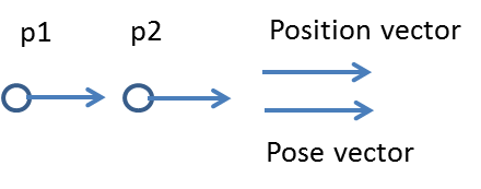
The observations $\mathbf{x}$ consist of individual related features $\mathbf{x}_{i}$ , group level features $\mathbf{x}_{g}$ and collective features $\mathbf{x}_{0}$ . The individual observations $\mathbf{x}_{i}\in\mathbb{R}^{|\mathcal{P}|\times|\mathcal{H}|}$ include pose $\in\mathcal{P}$ and action $\in\mathcal{H}$ . $\mathbf{x}_{g}$ is the mean of the feature vectors of the group members while $\mathbf{x}_{0}$ is the mean of feature vectors of all the individuals. Note that only pose and action are not enough to discriminate between waiting and queue since all the members possess the same pose and action. To incorporate some discrimination, we additionally include a pose-position compatibility to $\mathbf{x}_{g}$ . The score is calculated for all the pairs $(i,j)$ of the group members and is defined as $|p^{T}(d_{i}-d_{j})|$ where $p$ is the pose vector corresponding to the statistical mode of the member poses and $d_{i}$ is the position of the $i^{th}$ member. Higher value of the score corresponds to queue since both the vectors are aligned in the same direction while waiting will have a low value because both the vectors are orthogonal to each other. This is illustrated in Figure 4. We append the mean value of the score values obtained for all the pairs of the group to $\mathbf{x}_{g}$ .

To learn a pose classifier, we fine-tune all the 19 layers of the VGG [27] network on PARSE-27k [28] pedestrian attribute dataset comprised of 27 thousand labeled training images. To account for inherent order in poses, we modify cross entropy loss by penalizing misclassification. The penalty is less for predicting nearby pose and high otherwise; For example, the penalty is less if the classifier predicts Right-Front for the true pose of Right while the penalty is high if the prediction is Left.

We employ the following procedure to estimate action. We fit lines separately on the x and y coordinates of the top-left and bottom right of the bounding box as a function of time over 20 frames and use the estimated slopes to learn a SVM classifier for atomic action classification. The reason for considering both top-left and bottom right coordinates of the bounding box is to capture the possible movement along the viewing direction of the camera (i.e. effect of approaching and receding).

7.3 Tracking performance

We assume that the detections per frame are available to us. We do not handle occlusion in this paper. Whenever any target returns back to the scene after occlusion, a new id is assigned to it. To evaluate the tracking performance, we consider the number of identity switches. We compare the tracking results with a baseline model present in our framework. It corresponds to the track association based on visual, spatial and velocity compatibility (first part of Eq. 4) only. The full model incorporates both track association and group association. The number of ID switches are given in Table 1. The total number of tracks in the dataset is 466. The decrease in the number of ID switches in the full model indicates the effectiveness of combined estimation of groups and tracks over independent track association.

Table 1: Table showing tracking performance

	Baseline model	Full model
ID Switches	22 (4.5%)	17 (3.7%)

7.4 Group detection performance

To evaluate the group detection performance, we use the following clustering measures which are commonly used: Purity [1], Rand Index [23] and Normalized mutual information (NMI) [33]. We compare with a baseline case present within our framework which corresponds to group association (second part of Eq. 4). The full model incorporates both track association and group association. The quantitative results are given in Table 2.

Table 2: Table showing group detection performance

Framework	Purity	Rand Index	NMI
Baseline	0.82	0.75	0.65
Full	0.89	0.81	0.72

Again, the higher values of the clustering measures in the full model indicates the effectiveness of combined estimation of groups and tracks over independent group detection.

7.5 Activity recognition performance

We compare the collective activity results with [2], [14],[8] and [7] in the Table 3. To ensure a fair comparison with [2] and [14], we divide the dataset into separate training and testing sets as suggested by them. We use leave-one-video-out method to compare with [8] as suggested. To compare with [7], we use four fold setup with the splits mentioned by [7]. The Figure 5 compares the confusion table of the proposed framework with that of [7]. To find the accuracy for the group activity, we first identify the correctly detected groups and estimate accuracy for group activity on these groups. The confusion tables for group activity and atomic action are also given in Figure 5.

Table 3: Comparison of overall and mean accuracies

Accuracy	[2] $/$ [14] $/$ Ours			[8] $/$ Ours		[7] $/$ Ours
Overall	-	79.7	81.1	-	74.4	79.1	76.3
Mean Class	92.0	78.4	80.5	70.9	75.7	79.9	76.2

(a)

(b)

(c)

(d)

Figure 5: (a) Confusion matrix for collective activity

y

from [7]. (b), (c), (d) Confusion matrices for collective activity, group activity and atomic action respectively form the proposed method.

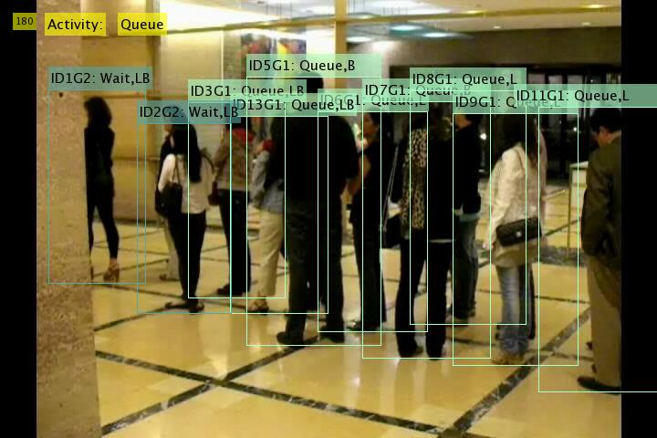
Form the Table 3, we notice that the proposed method offers a better accuracy than the methods [14] and [8], and is marginally inferior to [7]. However, all these methods assume availability of either tracklets or action labels whereas our method only needs the detections. Further, all these methods are non-causal in nature and involve batch processing of data unlike the proposed method. Additionally, we provide results at all levels of granularity (individual, group and collective). Figure 6 shows some qualitative results for group detection, group activity and collective activity. The members forming a group are represented by the same color. For example, Figure 6(a) has two groups which are correctly identified as crossing each other. Hence the group activity for both the groups is walking while the collective activity is crossing.

7.6 Computational Performance

Towards our main aim of developing a real-time system capable of simultaneous tracking, group detection and multi-level activity recognition, currently we achieve around 3 fps with our unoptimized MATLAB code on a i $7$ machine with $3.50$ GHz processor. With a proper implementation in GPU, we expect the frame rate to go up to 25 fps. To compare the computation time with one of the state-of-the-art algorithms, the method proposed in [2] takes 6 hours of training and 120 s per inference whereas our proposed method takes around 90 s and 0.3 s respectively.

8 Conclusions

In this paper, we have proposed a novel approach for video understanding at various levels of granularity. We have presented a linear programming based method for joint estimation of tracks and groups. We have also proposed a method to recognize activities at various levels - individual, group and collective. The framework being causal in nature and computationally efficient, it is amenable for real-time implementation in video surveillance applications. The experiments show that the proposed method is very competitive with the state-of-the-art algorithms.

References

[1] C. C. Aggarwal. A human-computer interactive method for projected clustering. IEEE Transactions on Knowledge and Data Engineering, 16(4):448–460, 2004.
[2] M. R. Amer, P. Lei, and S. Todorovic. Hirf: Hierarchical random field for collective activity recognition in videos. In European Conference on Computer Vision, pages 572–585. Springer, 2014.
[3] M. R. Amer, D. Xie, M. Zhao, S. Todorovic, and S.-C. Zhu. Cost-sensitive top-down/bottom-up inference for multiscale activity recognition. In European Conference on Computer Vision, pages 187–200. Springer, 2012.
[4] A. Andriyenko and K. Schindler. Globally optimal multi-target tracking on a hexagonal lattice. In European Conference on Computer Vision, pages 466–479. Springer, 2010.
[5] L. Bazzani, M. Zanotto, M. Cristani, and V. Murino. Joint individual-group modeling for tracking. IEEE transactions on pattern analysis and machine intelligence, 37(4):746–759, 2015.
[6] J. Berclaz, F. Fleuret, E. Turetken, and P. Fua. Multiple object tracking using k-shortest paths optimization. IEEE transactions on pattern analysis and machine intelligence, 33(9):1806–1819, 2011.
[7] W. Choi and S. Savarese. A unified framework for multi-target tracking and collective activity recognition. In European Conference on Computer Vision, pages 215–230. Springer, 2012.
[8] W. Choi, K. Shahid, and S. Savarese. Learning context for collective activity recognition. In Computer Vision and Pattern Recognition (CVPR), 2011 IEEE Conference on, pages 3273–3280. IEEE, 2011.
[9] H. Jiang, S. Fels, and J. J. Little. A linear programming approach for multiple object tracking. In Computer Vision and Pattern Recognition, 2007. CVPR’07. IEEE Conference on, pages 1–8. IEEE, 2007.
[10] T. Joachims, T. Finley, and C.-N. J. Yu. Cutting-plane training of structural svms. Machine Learning, 77(1):27–59, 2009.
[11] S. M. Khan and M. Shah. Detecting group activities using rigidity of formation. In Proceedings of the 13th annual ACM international conference on Multimedia, pages 403–406. ACM, 2005.
[12] T. Lan, L. Sigal, and G. Mori. Social roles in hierarchical models for human activity recognition. In Computer Vision and Pattern Recognition (CVPR), 2012 IEEE Conference on, pages 1354–1361. IEEE, 2012.
[13] T. Lan, Y. Wang, W. Yang, and G. Mori. Beyond actions: Discriminative models for contextual group activities. In Advances in neural information processing systems, pages 1216–1224, 2010.
[14] T. Lan, Y. Wang, W. Yang, S. N. Robinovitch, and G. Mori. Discriminative latent models for recognizing contextual group activities. IEEE Transactions on Pattern Analysis and Machine Intelligence, 34(8):1549–1562, 2012.
[15] L. Leal-Taixé, G. Pons-Moll, and B. Rosenhahn. Everybody needs somebody: Modeling social and grouping behavior on a linear programming multiple people tracker. In Computer Vision Workshops (ICCV Workshops), 2011 IEEE International Conference on, pages 120–127. IEEE, 2011.
[16] R. Li, R. Chellappa, and S. K. Zhou. Learning multi-modal densities on discriminative temporal interaction manifold for group activity recognition. In Computer Vision and Pattern Recognition, 2009. CVPR 2009. IEEE Conference on, pages 2450–2457. IEEE, 2009.
[17] J. Liu, J. Luo, and M. Shah. Recognizing realistic actions from videos “in the wild”. In Computer vision and pattern recognition, 2009. CVPR 2009. IEEE conference on, pages 1996–2003. IEEE, 2009.
[18] J. C. Niebles, H. Wang, and L. Fei-Fei. Unsupervised learning of human action categories using spatial-temporal words. International journal of computer vision, 79(3):299–318, 2008.
[19] S. Pellegrini, A. Ess, and L. Van Gool. Improving data association by joint modeling of pedestrian trajectories and groupings. In European Conference on Computer Vision, pages 452–465. Springer, 2010.
[20] H. Pirsiavash, D. Ramanan, and C. C. Fowlkes. Globally-optimal greedy algorithms for tracking a variable number of objects. In Computer Vision and Pattern Recognition (CVPR), 2011 IEEE Conference on, pages 1201–1208. IEEE, 2011.
[21] R. Poppe. A survey on vision-based human action recognition. Image and vision computing, 28(6):976–990, 2010.
[22] Z. Qin and C. R. Shelton. Improving multi-target tracking via social grouping. In Computer Vision and Pattern Recognition (CVPR), 2012 IEEE Conference on, pages 1972–1978. IEEE, 2012.
[23] W. M. Rand. Objective criteria for the evaluation of clustering methods. Journal of the American Statistical association, 66(336):846–850, 1971.
[24] M. Ryoo and J. Aggarwal. Stochastic representation and recognition of high-level group activities. International journal of computer Vision, 93(2):183–200, 2011.
[25] M. S. Ryoo and J. K. Aggarwal. Spatio-temporal relationship match: Video structure comparison for recognition of complex human activities. In Computer vision, 2009 ieee 12th international conference on, pages 1593–1600. IEEE, 2009.
[26] S. Savarese, A. DelPozo, J. C. Niebles, and L. Fei-Fei. Spatial-temporal correlatons for unsupervised action classification. In Motion and video Computing, 2008. WMVC 2008. IEEE Workshop on, pages 1–8. IEEE, 2008.
[27] K. Simonyan and A. Zisserman. Very deep convolutional networks for large-scale image recognition. CoRR, abs/1409.1556, 2014.
[28] P. Sudowe, H. Spitzer, and B. Leibe. Person Attribute Recognition with a Jointly-trained Holistic CNN Model. In ICCV’15 ChaLearn Looking at People Workshop, 2015.
[29] I. Tsochantaridis, T. Hofmann, T. Joachims, and Y. Altun. Support vector machine learning for interdependent and structured output spaces. In Proceedings of the twenty-first international conference on Machine learning, page 104. ACM, 2004.
[30] P. Turaga, R. Chellappa, V. S. Subrahmanian, and O. Udrea. Machine recognition of human activities: A survey. IEEE Transactions on Circuits and Systems for Video Technology, 18(11):1473–1488, 2008.
[31] L. Wang, Y. Qiao, and X. Tang. Latent hierarchical model of temporal structure for complex activity classification. IEEE Transactions on Image Processing, 23(2):810–822, 2014.
[32] D. Weinland, R. Ronfard, and E. Boyer. A survey of vision-based methods for action representation, segmentation and recognition. Computer vision and image understanding, 115(2):224–241, 2011.
[33] M. Wu and B. Schölkopf. A local learning approach for clustering. In Advances in neural information processing systems, pages 1529–1536, 2006.
[34] K. Yamaguchi, A. C. Berg, L. E. Ortiz, and T. L. Berg. Who are you with and where are you going? In Computer Vision and Pattern Recognition (CVPR), 2011 IEEE Conference on, pages 1345–1352. IEEE, 2011.
[35] L. Zhang, Y. Li, and R. Nevatia. Global data association for multi-object tracking using network flows. In Computer Vision and Pattern Recognition, 2008. CVPR 2008. IEEE Conference on, pages 1–8. IEEE, 2008.