On the dimension and smoothness of radial projectionsThanks: T.O. is supported by the Academy of Finland via the project Quantitative rectifiability in Euclidean and non-Euclidean spaces, grant number 309365. The research was also partially supported by travel grants from the Väisälä fund and Mathematics fund of the Finnish Academy of Science and Letters.

Tuomas Orponen Address: University of Helsinki, Department of Mathematics and Statistics Email address: tuomas.orponen@helsinki.fi

Abstract.

This paper contains two results on the dimension and smoothness of radial projections of sets and measures in Euclidean spaces.

To introduce the first one, assume that $E,K\subset\mathbb{R}^{2}$ are non-empty Borel sets with $\dim_{\mathrm{H}}K>0$ . Does the radial projection of $K$ to some point in $E$ have positive dimension? Not necessarily: $E$ can be zero-dimensional, or $E$ and $K$ can lie on a common line. I prove that these are the only obstructions: if $\dim_{\mathrm{H}}E>0$ , and $E$ does not lie on a line, then there exists a point in $x\in E$ such that the radial projection $\pi_{x}(K)$ has Hausdorff dimension at least $(\dim_{\mathrm{H}}K)/2$ . Applying the result with $E=K$ gives the following corollary: if $K\subset\mathbb{R}^{2}$ is Borel set, which does not lie on a line, then the set of directions spanned by $K$ has Hausdorff dimension at least $(\dim_{\mathrm{H}}K)/2$ .

For the second result, let $d\geq 2$ and $d-1<s<d$ . Let $\mu$ be a compactly supported Radon measure in $\mathbb{R}^{d}$ with finite $s$ -energy. I prove that the radial projections of $\mu$ are absolutely continuous with respect to $\mathcal{H}^{d-1}$ for every centre in $\mathbb{R}^{d}\setminus\operatorname{spt}\mu$ , outside an exceptional set of dimension at most $2(d-1)-s$ . In fact, for $x$ outside an exceptional set as above, the proof shows that $\pi_{x\sharp}\mu\in L^{p}(S^{d-1})$ for some $p>1$ . The dimension bound on the exceptional set is sharp.

Key words and phrases:

Hausdorff dimension, fractals, radial projections, visibility

2010 Mathematics Subject Classification

28A80 (Primary) 28A78 (Secondary)

1. Introduction

This paper studies visibility and radial projections. Given $x\in\mathbb{R}^{d}$ , define the radial projection $\pi_{x}\colon\mathbb{R}^{d}\setminus\{x\}\to S^{d-1}$ by

\pi_{x}(y)=\frac{y-x}{|y-x|}.

A Borel set $K\subset\mathbb{R}^{2}$ will be called

•

invisible from $x$ , if $\mathcal{H}^{d-1}(\pi_{x}(K\setminus\{x\}))=0$ , and
•

totally invisible from $x$ , if $\dim_{\mathrm{H}}\pi_{x}(K\setminus\{x\})=0$ .

Above, $\dim_{\mathrm{H}}$ and $\mathcal{H}^{s}$ stand for Hausdorff dimension and $s$ -dimensional Hausdorff measure, respectively. I will only consider Hausdorff dimension in this paper, as many of the results below would be much easier for box dimension. The study of (in-)visibility has a long tradition in geometric measure theory. For many more results and questions than I can introduce here, see Section 6 of Mattila’s survey [11]. The basic question is the following: given a Borel set $K\subset\mathbb{R}^{d}$ , how large can the sets

\mathrm{Inv}(K)=\{x\in\mathbb{R}^{d}:K\text{ is invisible from }x\}

and

\mathrm{Inv}_{T}(K):=\{x\in\mathbb{R}^{d}:K\text{ is totally invisible from }x\}

be? Clearly $\mathrm{Inv}_{T}(K)\subset\mathrm{Inv}(K)$ , and one generally expects $\mathrm{Inv}_{T}(K)$ to be significantly smaller than $\mathrm{Inv}(K)$ . The existing results fall roughly into the following three categories:

(1)

What happens if $\dim_{\mathrm{H}}K>d-1$ ?
(2)

What happens if $\dim_{\mathrm{H}}K\leq d-1$ ?
(3)

What happens if $0<\mathcal{H}^{d-1}(K)<\infty$ ?

Cases (1) and (3) are the most classical, having already been studied (for $d=2$ ) in the 1954 paper [8] of Marstrand. Given $s>1$ , Marstrand proved that any Borel set $K\subset\mathbb{R}^{2}$ with $0<\mathcal{H}^{s}(K)<1$ is visible (that is, not invisible) from Lebesgue almost every point $x\in\mathbb{R}^{2}$ , and also from $\mathcal{H}^{s}$ almost every point $x\in K$ . Unifying Marstrand’s results, and their generalisations to $\mathbb{R}^{d}$ , the following sharp bound was recently established by Mattila and the author in [13] and [14]:

(1.1)

\dim_{\mathrm{H}}\mathrm{Inv}(K)\leq 2(d-1)-\dim_{\mathrm{H}}K,

for all Borel sets $K\subset\mathbb{R}^{d}$ with $d-1<\dim_{\mathrm{H}}K\leq d$ . This paper contains a variant of the bound (1.1) for measures, see Section 1.2.

The visibility of sets $K$ in Case (3) depends on their rectifiability. I will restrict the discussion to the case $d=2$ for now. It is easy to show that $1$ -rectifiable sets, which are not $\mathcal{H}^{1}$ almost surely covered by a single line, are visible from all points in $\mathbb{R}^{2}$ , with possibly one exception, see [15]. On the other hand, if $K\subset\mathbb{R}^{2}$ is purely $1$ -unrectifiable, then the sharp bound

\dim_{\mathrm{H}}[\mathbb{R}^{2}\setminus\mathrm{Inv}(K)]=\dim_{\mathrm{H}}\{x\in\mathbb{R}^{2}:K\text{ is visible from }x\}\leq 1.

was obtained by Marstrand, building on Besicovitch’s projection theorem. For generalisations, improvements and constructions related to the bound above, see [9, Theorem 5.1], and [3, 4]. Marstrand raised the question – which remains open to the best of my knowledge – whether it is possible that $\mathcal{H}^{1}(\mathbb{R}^{2}\setminus\mathrm{Inv}(K))>0$ : in particular, can a purely $1$ -unrectifiable set be visible from a positive fraction of its own points? For purely $1$ -unrectifiable self-similar sets $K\subset\mathbb{R}^{2}$ one has $\mathrm{Inv}(K)=\mathbb{R}^{2}$ , as shown by Simon and Solomyak [17].

1.1. The first main result

Case (2) has received less attention. To simplify the discussion, assume that $\dim_{\mathrm{H}}K=1$ and $\mathcal{H}^{1}(K)=0$ , so that $\mathrm{Inv}(K)=\mathbb{R}^{2}$ , and the relevant question becomes the size of $\mathrm{Inv}_{T}(K)$ . The radial projections $\pi_{p}$ fit the influential generalised projections framework of Peres and Schlag [16]. If $K\subset\mathbb{R}^{2}$ is a Borel set with arbitrary dimension $s\in[0,2]$ , then it follows from [16, Theorem 7.3] that

(1.2)

\dim_{\mathrm{H}}\mathrm{Inv}_{T}(K)\leq 2-s.

When $s>1$ , the bound (1.2) is a weaker version of (1.1), but the benefit of (1.2) is that it holds without any restrictions on $s$ . In particular, if $s=1$ , one obtains

(1.3)

\dim_{\mathrm{H}}\mathrm{Inv}_{T}(K)\leq 1.

This bound is sharp for a trivial reason: consider the case, where $K$ lies on a single line $\ell\subset\mathbb{R}^{2}$ . Then, $\mathrm{Inv}_{T}(K)=\ell$ . The starting point for this paper was the question: are there essentially different examples manifesting the sharpness of (1.3)? The answer turns out to be negative in a very strong sense. Here are the first main results of the paper:

Theorem 1.4 (Weak version).

Assume that $K\subset\mathbb{R}^{2}$ is a Borel set with $\dim_{\mathrm{H}}K>0$ . Then, at least one of the following holds:

•

$\dim_{\mathrm{H}}\mathrm{Inv}_{T}(K)=0$ .
•

$\mathrm{Inv}_{T}(K)$ is contained on a line.

In fact, more is true. For $K\subset\mathbb{R}^{2}$ , define

\mathrm{Inv}_{1/2}(K):=\left\{x\in\mathbb{R}^{2}:\dim_{\mathrm{H}}\pi_{x}(K\setminus\{x\})<\tfrac{\dim_{\mathrm{H}}K}{2}\right\}.

Then, if $\dim_{\mathrm{H}}K>0$ , one evidently has $\mathrm{Inv}_{T}(K)\subset\mathrm{Inv}_{1/2}(K)\subset\mathrm{Inv}(K)$ .

Theorem 1.5 (Strong version).

Theorem 1.4 holds with $\mathrm{Inv}_{T}(K)$ replaced by $\mathrm{Inv}_{1/2}(K)$ . That is, if $E\subset\mathbb{R}^{2}$ is a Borel set with $\dim_{\mathrm{H}}E>0$ , not contained on a line, then there exists $x\in E$ such that $\dim_{\mathrm{H}}\pi_{x}(K\setminus\{x\})\geq(\dim_{\mathrm{H}}K)/2$ .

Remark 1.6.

A closely related result is Theorem 1.6 in the paper [1] of Bond, Łaba and Zahl; with some imagination, Theorem 1.6(a) in [1] can be viewed as a "single scale" variant of Theorem 1.5, although at this scale, Theorem 1.6(a) contains more information than Theorem 1.5. As far as I can tell, proving the Hausdorff dimension statement in this context presents a substantial extra challenge, so Theorem 1.5 is not easily implied by the results in [1].

Example 1.7.

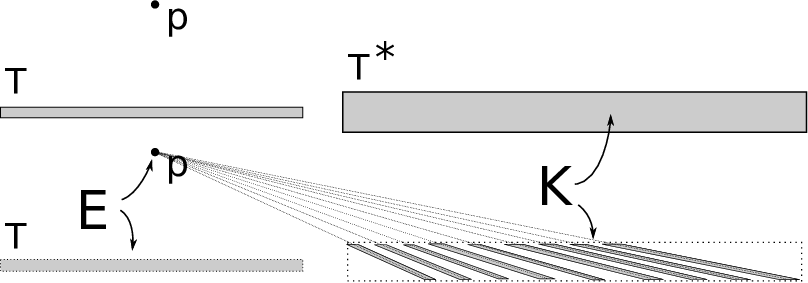
Figure 1 depicts the main challenge in the proofs of Theorems 1.4 and 1.5.

Refer to caption — Figure 1. What is the next step in the construction of $E$ ?

The set $E$ has $\dim_{\mathrm{H}}E>0$ , and consists of something inside a narrow tube $T$ , plus a point $x\notin T$ . Then, Theorem 1.4 states that $E\not\subset\mathrm{Inv}_{T}(K)$ for any compact set $K\subset\mathbb{R}^{2}$ with $\dim_{\mathrm{H}}K>0$ . So, in order to find a counterexample to Theorem 1.5, all one needs to do is find $K$ by a standard "Venetian blind" construction, in such a way that $\dim_{\mathrm{H}}K>0$ and $\dim_{\mathrm{H}}\pi_{y}(K)=0$ for all $y\in E$ . The first steps are obvious: to begin with, require that $K\subset T^{\ast}$ for another narrow tube parallel to $T$ , see Figure 1. Then $\pi_{y}(K)$ is small for all $y\in T$ . To handle the special point $x\in E$ , split the contents of $T^{\ast}$ into a finite collection of new narrow tubes in such a way that $\pi_{x}(K)$ is small. In this manner, $\pi_{y}(K)$ can be made arbitrarily small for all $y\in E$ (in the sense of $\epsilon$ -dimensional Hausdorff content, for instance, for any prescribed $\epsilon>0$ ). It is quite instructive to think, why the construction cannot be completed: why cannot the "Venetian blinds" be iterated further (for both $E$ and $K$ ) so that, at the limit, $\dim_{\mathrm{H}}\pi_{y}(K)=0$ for all $x\in E$ ?

Theorem 1.5 has the following immediate consequence:

Corollary 1.8 (Corollary to Theorem 1.5).

Assume that $K\subset\mathbb{R}^{2}$ is a Borel set, not contained on a line. Then the set of unit vectors spanned by $K$ , namely

S(K):=\left\{\tfrac{x-y}{|x-y|}\in S^{1}:x,y\in K\text{ and }x\neq y\right\},

satisfies $\dim_{\mathrm{H}}S(K)\geq\tfrac{\dim_{\mathrm{H}}K}{2}$ .

Proof.

If $\dim_{\mathrm{H}}K=0$ , there is nothing to prove. Otherwise, Theorem 1.5 implies that $K\not\subset\mathrm{Inv}_{1/2}(K)$ , whence $\dim_{\mathrm{H}}S(K)\geq\dim_{\mathrm{H}}\pi_{x}(K\setminus\{x\})\geq(\dim_{\mathrm{H}}K)/2$ for some $x\in K$ . ∎

Corollary 1.8 is probably not sharp, and the following conjecture seems plausible:

Conjecture 1.9.

Assume that $K\subset\mathbb{R}^{2}$ is a Borel set, not contained on a line. Then $\dim_{\mathrm{H}}S(K)=\min\{\dim_{\mathrm{H}}K,1\}$ .

This follows from Marstrand’s result, discussed in Case (1) above, when $\dim_{\mathrm{H}}K>1$ . For $\dim_{\mathrm{H}}K\leq 1$ , Conjecture 1.9 is closely connected with continuous sum-product problems, which means that significant improvements over Corollary 1.8 will, most likely, require new technology. It would, however, be interesting to know if an $\epsilon$ -improvement over Corollary 1.8 is possible, combining the proof below with ideas from the paper [6] of Katz and Tao, and using the discretised sum-product theorem of Bourgain [2].

I have the referee to thank for pointing out that a natural discrete variant of Conjecture 1.9 has been solved by P. Ungar [18] as early as 1982: a set of $n\geq 3$ points in the plane, not all on a single line, determine at least $n-1$ distinct directions.

1.2. The second main result

The second main result is a version of the estimate (1.1) for measures. Fix $d\geq 2$ , and denote the space of compactly supported Radon measures on $\mathbb{R}^{d}$ is denoted by $\mathcal{M}(\mathbb{R}^{d})$ . For $\mu\in\mathcal{M}(\mathbb{R}^{d})$ , write

\mathcal{S}(\mu):=\{x\in\mathbb{R}^{d}\setminus\operatorname{spt}\mu:\pi_{x\sharp}\mu\text{ is not absolutely continuous w.r.t. }\mathcal{H}^{d-1}|_{S^{d-1}}\}.

Note that whenever $x\in\mathbb{R}^{d}\setminus\operatorname{spt}\mu$ , the projection $\pi_{x}$ is continuous on $\operatorname{spt}\mu$ , and $\pi_{x\sharp}\mu$ is well-defined. One can check that the family of projections $\{\pi_{x}\}_{x\in\mathbb{R}^{d}\setminus\operatorname{spt}\mu}$ fits in the generalised projections framework of Peres and Schlag [16], and indeed Theorem 7.3 in [16] yields

(1.10)

\dim_{\mathrm{H}}\mathcal{S}(\mu)\leq 2d-1-s,

whenever $d-1<s<d$ and $\mu\in\mathcal{M}(\mathbb{R}^{d})$ has finite $s$ -energy (see (1.12) for a definition). Combining this bound with standard arguments shows that if $K\subset\mathbb{R}^{d}$ is a Borel set with $d-1<\dim_{\mathrm{H}}K\leq d$ , then

\dim_{\mathrm{H}}\mathrm{Inv}(K)=\dim_{\mathrm{H}}\{x\in\mathbb{R}^{d}:\mathcal{H}^{d-1}(\pi_{x}(K))=0\}\leq 2d-1-\dim_{\mathrm{H}}K.

This is weaker than the sharp bound (1.1), so it is a natural to ask, whether the bound (1.10) for measures could be lowered to match (1.1). The answer is affirmative:

Theorem 1.11.

If $\mu\in\mathcal{M}(\mathbb{R}^{d})$ and

(1.12)

I_{s}(\mu):=\iint\frac{d\mu(x)\,d\mu(y)}{|x-y|^{s}}<\infty

for some $s>d-1$ , then $\dim_{\mathrm{H}}\mathcal{S}(\mu)\leq 2(d-1)-s$ .

The bound is sharp, essentially because (1.1) is, and Theorem 1.11 implies (1.1). More precisely, following [14, Section 2.2], there exist compact sets $K\subset\mathbb{R}^{d}$ of any dimension $\dim_{\mathrm{H}}K\in(d-1,d)$ such that

\dim_{\mathrm{H}}[\mathrm{Inv}(K)\setminus K]=2(d-1)-\dim K.

Then, the sharpness of Theorem 1.11 follows by considering Frostman measures supported on $K$ , and noting that $\mathcal{S}(\mu)\supset\mathrm{Inv}(K)\setminus K$ whenever $\mu\in\mathcal{M}(\mathbb{R}^{d})$ and $\operatorname{spt}\mu\subset K$ .

An open question is the validity of Theorem 1.11 for $s=d-1$ . If $I_{d-1}(\mu)<\infty$ , Theorem 7.3 in [16] implies that $\mathcal{L}^{d}(\mathcal{S}(\mu))=0$ , but I do not even know if $\dim_{\mathrm{H}}\mathcal{S}(\mu)<d$ .

Theorem 1.11 does not immediately follow from the proof of (1.1) in [13] and [14], as the argument in those papers was somewhat indirect. Having said that, many observations from the previous papers still play a role in the new proof. Theorem 1.11 will be deduced from the next statement concerning $L^{p}$ -densities:

Theorem 1.13.

Let $\mu\in\mathcal{M}(\mathbb{R}^{d})$ as in Theorem 1.5. For $p\in(1,2)$ , write

\mathcal{S}_{p}(\mu):=\{x\in\mathbb{R}^{d}\setminus\operatorname{spt}\mu:\pi_{x\sharp}\mu\notin L^{p}(S^{d-1})\}.

Then $\dim_{\mathrm{H}}\mathcal{S}_{p}(\mu)\leq 2(d-1)-s+\delta(p)$ , where $\delta(p)>0$ , and $\delta(p)\to 0$ as $p\searrow 1$ .

Note that the claim is vacuous for "large" values of $p$ . The dependence of $\delta(p)>0$ on $p$ is effective and not very hard to track, see (3.5).

Remark 1.14.

Theorem 1.13 can be viewed as an extension of Falconer’s exceptional set estimate [5] from 1982. I only discuss the planar case. Falconer proved that if $I_{s}(\mu)<\infty$ for some $1<s<2$ , then the orthogonal projections of $\mu$ to all $1$ -dimensional subspaces are in $L^{2}$ , outside an exceptional set of dimension at most $2-s$ . Now, orthogonal projections can be viewed as radial projections from points on the line at infinity. Alternatively, if the reader prefers a more rigorous statement, Falconer’s proof shows that if $\ell\subset\mathbb{R}^{2}$ is any fixed line outside the support of $\mu$ , then all the radial projections of $\mu$ to points on $\ell$ are in $L^{2}$ , outside an exceptional set of dimension at most $2-s$ . In comparison, Theorem 1.13 states that the radial projections of $\mu$ to points in $\mathbb{R}^{2}\setminus\operatorname{spt}\mu$ are in $L^{p}$ for some $p>1$ , outside an exceptional set of dimension at most $2-s$ . So, the size of the exceptional set remains the same even if the "fixed line $\ell$ " is removed from the statement. The price to pay is that the projections only belong to some $L^{p}$ with $p>1$ (possibly) smaller than $2$ . I do not know, if the reduction in $p$ is necessary, or an artefact of the proof.

1.3. Acknowledgements

I started working on the questions while taking part in the research programme Fractal Geometry and Dynamics at Institut Mittag-Leffler. I am grateful to the organisers for letting me participate, and to the staff of the institute for making my stay very pleasant. I would also like to thank Tamás Keleti and Pablo Shmerkin for stimulating conversations, both on this project, and several related topics. I thank Pablo for explicitly asking, whether Theorem 1.11 is true. The visit at the institute was enabled financially by travel grants from the Väisälä fund and Mathematics fund of the Finnish Academy of Science and Letters.

I am grateful to the referee for a careful reading of the manuscript, and for many helpful suggestions.

2. Proof of Theorem 1.5

If $\ell\subset\mathbb{R}^{2}$ is a line, I denote by $T(\ell,\delta)$ the open (infinite) tube of width $2\delta$ , with $\ell$ "running through the middle", that is, $\operatorname{dist}(\ell,\mathbb{R}^{2}\setminus T(\ell,\delta))=\delta$ . The notation $B(x,r)$ stands for a closed ball with centre $x\in\mathbb{R}^{2}$ and radius $r>0$ . The notation $A\lesssim B$ means that there is an absolute constant $C\geq 1$ such that $A\leq CB$ .

Lemma 2.1.

Assume that $\mu$ is a Borel probability measure on $B(0,1)\subset\mathbb{R}^{2}$ , and $\mu(\ell)=0$ for all lines $\ell\subset\mathbb{R}^{2}$ . Then, for any $\epsilon>0$ , there exists $\delta>0$ such that $\mu(T(\ell,\delta))\leq\epsilon$ for all lines $\ell\subset\mathbb{R}^{2}$ .

Proof.

Assume not, so there exists $\epsilon>0$ , a sequence of positive numbers $\delta_{1}>\delta_{2}>\ldots>0$ with $\delta_{i}\searrow 0$ , and a sequence of lines $\{\ell_{i}\}_{i\in\mathbb{N}}\subset\mathbb{R}^{2}$ with $\mu(T(\ell_{i},\delta_{i}))\geq\epsilon$ . Since $\operatorname{spt}\mu\subset B(0,1)$ , one has $\ell_{i}\cap B(0,1)\neq\emptyset$ for all $i\in\mathbb{N}$ . Consequently, there exists a subsequence $(i_{j})_{j\in\mathbb{N}}$ , and a line $\ell\subset\mathbb{R}^{2}$ such that $\ell_{j}\to\ell$ in the Hausdorff metric. Then, for any given $\delta>0$ , there exists $j\in\mathbb{N}$ such that

B(0,1)\cap T(\ell_{i_{j}},\delta_{i_{j}})\subset T(\ell,\delta),

so that $\mu(T(\ell,\delta))\geq\epsilon$ . It follows that $\mu(\ell)\geq\epsilon$ , a contradiction. ∎

The next lemma contains all the information needed to prove Theorem 1.5. I state two versions: the first one is slightly easier to read and apply, while the second one is slightly more detailed.

Lemma 2.2.

Assume that $\mu,\nu$ are Borel probability measures with compact supports $K,E\subset B(0,1)$ , respectively. Assume that both measures $\mu$ and $\nu$ satisfy a Frostman condition with exponents $\kappa_{\mu},\kappa_{\nu}\in(0,2]$ , respectively:

(2.3)

\mu(B(x,r))\leq C_{\mu}r^{\kappa_{\mu}}\quad\text{and}\quad\nu(B(x,r))\leq C_{\nu}r^{\kappa_{\nu}}

for all balls $B(x,r)\subset\mathbb{R}^{2}$ , and for some constants $C_{\mu},C_{\nu}\geq 1$ . Assume further that $\mu(\ell)=0$ for all lines $\ell\subset\mathbb{R}^{2}$ . Fix also

0<\tau<\tfrac{\kappa_{\mu}}{2}\quad\text{and}\quad\epsilon>0,

and write $\delta_{k}:=2^{-(1+\epsilon)^{k}}$ .

Then, there exists a compact subset $K^{\prime}\subset K$ with

\mu(K^{\prime})\geq\frac{1}{2},

a number $\eta=\eta(\epsilon,\kappa_{\mu},\kappa_{\nu},\tau)>0$ , an index $k_{0}=k_{0}(\epsilon,\mu,\kappa_{\nu},\tau)\in\mathbb{N}$ , and a point $x\in E$ with the following property. If $k>k_{0}$ , and $T(\ell_{1},\delta_{k}),\ldots,T(\ell_{N},\delta_{k})$ is a family of $\delta_{k}$ -tubes of cardinality $N\leq\delta_{k}^{-\tau}$ , each containing $x$ , then

(2.4)

\mu\left(K^{\prime}\cap\bigcup_{j=1}^{N}T(\ell_{j},\delta_{k})\right)\leq\delta_{k}^{\eta}.

Roughly speaking, the conclusion (2.4) means that $K^{\prime}$ has a radial projection of dimension $\geq\tau$ relative to the viewpoint $x\in E$ , since only a tiny fraction of $K^{\prime}$ can be covered by $\leq\delta_{k}^{-\tau}$ tubes of width $2\delta_{k}$ containing $x$ .

The set $K^{\prime}\subset K$ and the point $x\in E$ will be found by induction on the scales $\delta_{k}$ . To set the scene for the induction, it is convenient to state a more detailed version of the lemma:

Lemma 2.5.

(2.6)

\mu(B(x,r))\leq C_{\mu}r^{\kappa_{\mu}}\quad\text{and}\quad\nu(B(x,r))\leq C_{\nu}r^{\kappa_{\nu}}

for all balls $B(x,r)\subset\mathbb{R}^{2}$ , and for some constants $C_{\mu},C_{\nu}\geq 1$ . Assume further that $\mu(\ell)=0$ for all lines $\ell\subset\mathbb{R}^{2}$ . Fix also

0<\tau<\tfrac{\kappa_{\mu}}{2}\quad\text{and}\quad\epsilon>0,

and write $\delta_{k}:=2^{-(1+\epsilon)^{k}}$ .

Then, there exist numbers $\beta=\beta(\kappa_{\mu},\kappa_{\nu},\tau)>0$ , $\eta=\eta(\epsilon,\kappa_{\mu},\kappa_{\nu},\tau)>0$ , and an index $k_{0}=k_{0}(\epsilon,\mu,\kappa_{\nu},\tau)\in\mathbb{N}$ with the following properties. For all $k\geq k_{0}$ , there exist

(a)

compact sets $K\supset K_{k_{0}}\supset K_{k_{0}+1}\ldots$ with

(2.7) $\mu(K_{k})\geq 1-\sum_{k_{0}\leq j<k}(\tfrac{1}{4})^{j-k_{0}+1}\geq\frac{1}{2},$
(b)

compact sets $E\supset E_{k_{0}}\supset E_{k_{0}+1}\ldots$ with $\nu(E_{k})\geq\delta_{k}^{\beta}$

with the following property: if $k>k_{0}$ , $x\in E_{k}$ , and $T(\ell_{1},\delta_{k}),\ldots,T(\ell_{N},\delta_{k})$ is a family of tubes of cardinality $N\leq\delta_{k}^{-\tau}$ , each containing $x$ , then

(2.8)

\mu\left(K_{k}\cap\bigcup_{j=1}^{N}T(\ell_{j},\delta_{k})\right)\leq\delta_{k}^{\eta}.

Remark 2.9.

The index $k_{0}$ can be chosen as large as desired; this will be clear from the proof below. It will also be used on many occasions, without separate remark, that $\delta_{k}$ can be assumed very small for all $k\geq k_{0}$ . I also record that Lemma 2.2 follows from Lemma 2.5: simply take $K^{\prime}$ to be the intersection of all the sets $K_{j}$ , $j\geq k_{0}$ , and let $x\in E$ be any point in the intersection of all the sets $E_{j}$ , $j\geq k_{0}$ .

Proof.

As stated above, the proof is by induction, starting at the largest scale $k_{0}$ , which will be presently defined. Fix $\eta=\eta(\epsilon,\kappa_{\mu},\kappa_{\nu},\tau)>0$ and

(2.10)

\Gamma=\Gamma(\epsilon,\kappa_{\mu},\kappa_{\nu},\tau)\in\mathbb{N}

The number $\Gamma$ will be specified at the very end of the proof, right before (2.35), and there will be several requirements for the number $\eta$ , see (2.25), (2.31), and (2.34). Applying Lemma 2.1, first pick an index $k_{1}=k_{1}(\epsilon,\mu,\kappa_{\nu},\tau)\in\mathbb{N}$ such that $\mu(T(\ell,\delta_{k_{1}}))\leq(\tfrac{1}{4})^{\Gamma+1}$ for all tubes $T(\ell,\delta_{k_{1}})\subset\mathbb{R}^{2}$ , and

(2.11)

\delta_{k-\Gamma}^{\eta}\leq(\tfrac{1}{4})^{k-\Gamma+1},\qquad k\geq k_{1}.

Set $k_{0}:=k_{1}+\Gamma$ . Then, the following holds for all $k\in\{k_{0},\ldots,k_{0}+\Gamma\}$ . For any subset $K^{\prime}\subset K$ , and any tube $T(\ell,\delta_{k-\Gamma})\subset\mathbb{R}^{2}$ , one has

(2.12)

\mu(K^{\prime}\cap T(\ell,\delta_{k-\Gamma}))\leq\mu(T(\ell,\delta_{k_{1}}))\leq(\tfrac{1}{4})^{\Gamma+1}\leq(\tfrac{1}{4})^{k-k_{0}+1}.

Define

K_{k}:=K\quad\text{and}\quad E_{k}:=E,\qquad k_{1}\leq k\leq k_{0}.

(The definitions of $E_{k},K_{k}$ for $k_{1}\leq k<k_{0}$ are only given for notational convenience.)

I start by giving an outline of how the induction will proceed. Assume that, for a certain $k\geq k_{0}$ , the sets $K_{k}$ and $E_{k}$ have been constructed such that

(i)

the condition (2.12) is satisfied with $K^{\prime}=K_{k}$ , and for all tubes $T(\ell,\delta_{k-\Gamma})$ with $T(\ell,\delta_{k-\Gamma})\cap E_{k-\Gamma}\neq\emptyset$ .
(ii)

$K_{k}$ and $E_{k}$ satisfy the measure lower bounds (a) and (b) from the statement of the lemma.

Under the conditions (i)-(ii), I claim that it is possible to find subsets $K_{k+1}\subset K_{k}$ and $E_{k+1}\subset E_{k}$ , satisfying (ii) at level $k+1$ , and also the non-concentration condition (2.8) at level $k+1$ . This is why (2.8) is only claimed to hold for $k>k_{0}$ , and no one is indeed claiming that it holds for the sets $K_{k_{0}}$ and $E_{k_{0}}$ . These sets satisfy (i), however, which should be viewed as a weaker substitute for (2.8) at level $k$ , which is just strong enough to guarantee (2.8) at level $k+1$ . There is one obvious question at this point: if (i) at level $k$ gives (2.8) at level $k+1$ , then where does one get (i) back at level $k+1$ ?

If $k+1\in\{k_{0},\ldots,k_{0}+\Gamma\}$ , the condition (i) is simply guaranteed by the choice of $k_{0}$ (one does not even need to assume that $T(\ell,\delta_{k-\Gamma})\cap E_{k-\Gamma}\neq\emptyset$ ). For $k+1>k_{0}+\Gamma$ , this is no longer true. However, for $k+1>\Gamma+k_{0}$ , one has $k+1-\Gamma>k_{0}$ , and thus $K_{k+1-\Gamma}$ and $E_{k+1-\Gamma}$ have already been constructed to satisfy (2.8). In particular, if $E_{k+1-\Gamma}\cap T(\ell,\delta_{k+1-\Gamma})\neq\emptyset$ , then

(2.13)

\mu(K_{k+1}\cap T(\ell,\delta_{k+1-\Gamma}))\leq\mu(K_{k+1-\Gamma}\cap T(\ell,\delta_{k+1-\Gamma}))\leq\delta_{k+1-\Gamma}^{\eta}\leq(\tfrac{1}{4})^{(k+1)-k_{0}+1}

by (2.8) and (2.11). This means that (i) is satisfied at level $k+1$ , and the induction may proceed.

So, it remains to prove that (i)–(ii) at level $k$ imply (ii) and (2.8) at level $k+1$ . To avoid clutter, I write

\delta:=\delta_{k+1}.

Assume that the sets $K_{k},E_{k}$ have been constructed for some $k\geq k_{0}$ , satisfying (i)–(ii). The main task is to understand the structure of the set of points $x\in E_{k}$ for which (2.8) fails. To this end, we define the set $\textbf{Bad}_{k}\subset E_{k}$ as follows: $x\in\textbf{Bad}_{k}$ , if and only if $x\in E_{k}$ , and there exist $N\leq\delta^{-\tau}$ tubes $T(\ell_{1},\delta),\ldots,T(\ell_{N},\delta)$ , each containing $x$ , such that

(2.14)

\mu\left(K_{k}\cap\bigcup_{j=1}^{N}T(\ell_{j},\delta)\right)>\delta^{\eta}.

Note that if $\textbf{Bad}_{k}=\emptyset$ , then one can simply define $E_{k+1}:=E_{k}$ and $K_{k+1}:=K_{k}$ , and (ii) and (2.8) (at level $k+1$ ) are clearly satisfied.

Instead of analysing $\textbf{Bad}_{k}$ directly, it is useful to split it up into "directed" pieces, and digest the pieces individually. To make this precise, let $S$ be the "space of directions"; for concreteness, I identify $S$ with the upper half of the unit circle. Then, if $T=T(\ell,\delta)\subset\mathbb{R}^{2}$ is a tube, I denote by $\textup{dir}(T)$ the unique vector $e\in S$ such that $\ell\|e$ .

Recall the small parameter $\eta>0$ , and partition $S$ into $D=\delta^{-\eta}$ arcs $J_{1},\ldots,J_{D}$ of length $\sim\delta^{\eta}$ .¹¹ 1 Here, it might be better style to pick another letter, say $\alpha>0$ , in place of $\eta$ , since the two parameters play slightly different roles in the proof. Eventually, however, one would end up considering $\min\{\eta,\alpha\}$ , and it seems a bit cleaner to let $\eta>0$ be a ”jack of all trades” from the start. For $d\in\{1,\ldots,D\}$ fixed (" $d$ " for "direction"), consider the set $\textbf{Bad}_{k}^{d}$ : it consists of those points $x\in E_{k}$ such that there exist $N\leq\delta^{-\tau}$ tubes $T(\ell_{1},\delta),\ldots,T(\ell_{N},\delta)$ , each containing $x$ , with $\textup{dir}(T(\ell_{i},\delta))\in J_{d}$ , and satisfying

\mu\left(K_{k}\cap\bigcup_{j=1}^{N}T(\ell_{j},\delta)\right)>\delta^{2\eta}.

Since the direction of every possible tube in $\mathbb{R}^{2}$ belongs to one of the arcs $J_{i}$ , and there are only $D=\delta^{-\eta}$ arcs in total, one has

(2.15)

\textbf{Bad}_{k}\subset\bigcup_{d=1}^{D}\textbf{Bad}_{k}^{d}.

The next task is to understand the structure of $\textbf{Bad}_{k}^{d}$ for a fixed direction $d\in\{1,\ldots,D\}$ . I claim that $\textbf{Bad}_{k}^{d}$ looks like a garden of flowers, with all the petals pointing in direction $J_{d}$ , see Figure 2 for a rough idea.

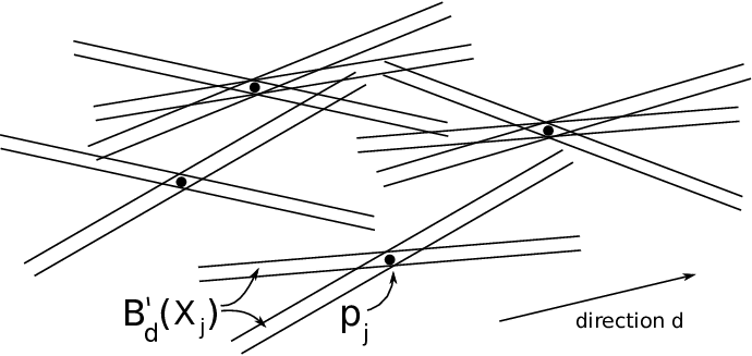
To make the statement more precise, I introduce an additional piece of notation. Fox $X\subset K_{k}$ , let $B_{d}(X)$ consist of those points $x\in E_{k}$ such that $X$ can be covered by $N\leq\delta^{-\tau}$ tubes $T(\ell_{1},\delta),\ldots,T(\ell_{N},\delta)$ , with directions $\textup{dir}(T(\ell_{i},\delta))\in J_{d}$ , and each containing $x$ . Then, note that

(2.16)

\textbf{Bad}_{k}^{d}=\{x\in E_{k}:\exists\,X\subset K_{k}\text{ with }\mu(X)>\delta^{2\eta}\text{ and }x\in B_{d}(X)\}.

The sets $B_{d}(X)$ also have the trivial but useful property that

X\subset X^{\prime}\subset K_{k}\quad\Longrightarrow\quad B_{d}(X^{\prime})\subset B_{d}(X).

There are two steps in establishing the "garden" structure of $\textbf{Bad}_{k}^{d}$ : first, one needs to find the "flowers", and second, one needs to check that the sets obtained actually look like flowers in a non-trivial sense. I start with the former task. Assuming that $\textbf{Bad}_{k}^{d}\neq\emptyset$ , pick any point $x_{1}\in\textbf{Bad}_{k}^{d}$ , and an associated subset $X_{1}\subset K_{k}$ with

\mu(X_{1})>\delta^{2\eta}\quad\text{and}\quad x_{1}\in B_{d}(X_{1}).

Then, assume that $x_{1},\ldots,x_{m}\in\textbf{Bad}_{k}^{d}$ and $X_{1},\ldots,X_{m}$ have already been chosen with the properties above, and further satisfying

(2.17)

\mu(X_{i}\cap X_{j})\leq\delta^{4\eta}/2,\qquad 1\leq i<j\leq m.

Then, see if there still exists a subset $X_{m+1}\subset K_{k}$ with the following three properties: $\mu(X_{m+1})>\delta^{2\eta}$ , $B_{d}(X_{m+1})\neq\emptyset$ , and $\mu(X_{m+1}\cap X_{i})\leq\delta^{4\eta}/2$ for all $1\leq i\leq m$ . If such a set no longer exists, stop; if it does, pick $x_{m+1}\in B_{d}(X_{m+1})$ , and add $X_{m+1}$ to the list.

It follows from the "competing" conditions $\mu(X_{i})>\delta^{2\eta}$ , and (2.17), that the algorithm needs to terminate in at most

(2.18)

M\leq 2\delta^{-4\eta}

Indeed, assume that the sets $X_{1},\ldots,X_{M}$ have already been constructed, and consider the following chain of inequalities:

	$\displaystyle\frac{1}{M}+\frac{1}{M(M-1)}\sum_{i_{1}\neq i_{2}}\mu(X_{i_{1}}\cap X_{i_{2}})$	$\displaystyle\geq\frac{1}{M^{2}}\sum_{i_{1},i_{2}=1}^{M}\mu(X_{i_{1}}\cap X_{i_{2}})$
		$\displaystyle=\frac{1}{M^{2}}\int\sum_{i_{1},i_{2}=1}^{M}\mathbf{1}_{X_{i_{1}}\cap X_{i_{2}}}(x)\,d\mu(x)$
		$\displaystyle=\frac{1}{M^{2}}\int[\operatorname{card}\{1\leq i\leq M:x\in X_{i}\}]^{2}\,d\mu(x)$
		$\displaystyle\geq\frac{1}{M^{2}}\left(\int\operatorname{card}\{1\leq i\leq M:x\in X_{i}\}\,d\mu(x)\right)^{2}$
		$\displaystyle=\frac{1}{M^{2}}\left(\sum_{i=1}^{M}\mu(X_{i})\right)^{2}>\delta^{4\eta}.$

Thus, if $M>2\delta^{-4\eta}$ , there exists a pair $X_{i_{1}},X_{i_{2}}$ with $i_{1}\neq i_{2}$ such that $\mu(X_{i_{1}}\cap X_{i_{2}})>\delta^{4\eta}/2$ , and the algorithm has already terminated earlier. This proves (2.18).

With the sets $X_{1},\ldots,X_{M}$ now defined, write

B_{d}^{\prime}(X_{j}):=\{x\in E_{k}:\exists\,X^{\prime}\subset X_{j}\text{ with }\mu(X^{\prime})>\delta^{4\eta}/2\text{ and }p\in B_{d}(X^{\prime})\}.

I claim that

(2.19)

\textbf{Bad}_{k}^{d}\subset\bigcup_{j=1}^{M}B_{d}^{\prime}(X_{j}).

Indeed, if $x\in\textbf{Bad}_{k}^{d}$ , then $x\in B_{d}(X)$ for some $X\subset K_{k}$ with $\mu(X)>\delta^{2\eta}$ by (2.16). It follows that

(2.20)

\mu(X\cap X_{j})>\delta^{4\eta}/2

for one of the sets $X_{j}$ , $1\leq j\leq M$ , because either $X\in\{X_{1},\ldots,X_{M}\}$ , and (2.20) is clear (all the sets $X_{j}$ even satisfy $\mu(X_{j})>\delta^{2\eta}$ ), or else (2.20) must hold by virtue of $X$ not having been added to the list $X_{1},\ldots,X_{M}$ in the algorithm. But (2.20) implies that $x\in B_{d}^{\prime}(X_{j})$ , since $X^{\prime}=X\cap X_{j}\subset X_{j}$ satisfies $\mu(X^{\prime})>\delta^{4\eta}/2$ and $x\in B_{d}(X)\subset B_{d}(X^{\prime})$ .

According to (2.18) and (2.19) the set $\textbf{Bad}_{k}^{d}$ can be covered by $M\leq 2\delta^{-4\eta}$ sets of the form $B_{d}^{\prime}(X_{j})$ , see Figure 2. These sets are the "flowers", and their structure is explored in the next lemma:

Lemma 2.21.

The following holds, if $\delta=\delta_{k+1}$ and $\eta>0$ are small enough (the latter depending on $\kappa_{\mu},\tau$ here). For $1\leq d\leq D$ and $1\leq j\leq M$ fixed, the set $B_{d}^{\prime}(X_{j})$ can be covered by $\leq 4\delta^{-8\eta}$ tubes of the form $T=T(\ell,\delta^{\rho})$ , where $\textup{dir}(T)\in J_{d}$ , and $\rho=\rho(\kappa_{\mu},\tau)>0$ . The tubes can be chosen to contain the point $x_{j}\in B_{d}(X_{j})$ .

Proof.

Fix $1\leq j\leq M$ and $x\in B_{d}^{\prime}(X_{j})$ . Recall the point $x_{j}\in B_{d}(X_{j})$ from the definition of $X_{j}$ . By definition of $x\in B_{d}^{\prime}(X_{j})$ , there exists a set $X^{\prime}\subset X_{j}$ with $\mu(X^{\prime})>\delta^{4\eta}/2$ and $x\in B_{d}(X^{\prime})$ . Unwrapping the definitions further, there exist $N\leq\delta^{-\tau}$ tubes $T(\ell_{1},\delta),\ldots,T(\ell_{N},\delta)$ , the union of which covers $X^{\prime}$ , and each satisfies $\textup{dir}(T(\ell_{i},\delta))\in J_{d}$ and $x\in T(\ell_{i},\delta)$ . In particular, one of these tubes, say $T_{x}=T(\ell_{i},\delta)$ , has

(2.22)

\mu(X_{j}\cap T_{x})\geq\mu(X^{\prime}\cap T_{x})\geq\mu(X^{\prime})\cdot\delta^{\tau}\geq\delta^{4\eta+\tau}/2\geq\delta^{8\eta+\tau}/4.

(The final inequality is just a triviality at this point, but is useful for later technical purposes later.) Here comes perhaps the most basic geometric observation in the proof: if the measure lower bound (2.22) holds for some $\delta$ -tube $T$ – this time $T_{x}$ – and a sufficiently small $\eta>0$ (crucially so small that $8\eta+\tau<\kappa_{\mu}/2$ ), then the whole set $B_{d}(X_{j})$ is actually contained in a neighbourhood of $T$ , called $T^{\ast}$ , because $X_{j}\cap T$ is so difficult to cover by $\delta$ -tubes centred at points outside $T^{\ast}$ , see Figure 3.

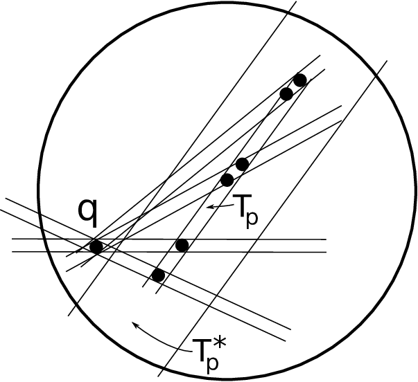
In particular, in the present case,

(2.23)

x_{j}\in B_{d}(X_{j})\subset T(\ell_{i},\delta^{4\rho})=:T_{x}^{\ast}

for a suitable constant $\rho=\rho(\kappa_{\mu},\tau)>0$ , specified in (2.25). To see this formally, pick $y\in B(0,1)\setminus T_{x}^{\ast}$ , and argue as follows to show that $y\notin B_{d}(X_{j})$ . First, any $\delta$ -tube $T$ containing $y$ , and intersecting $T_{x}\cap B(0,1)$ , makes an angle of at least $\gtrsim\delta^{4\rho}$ with $T_{x}$ . It follows that

\operatorname{diam}(T\cap T_{x}\cap B(0,1))\lesssim\delta^{1-4\rho},

and consequently $\mu(T\cap T_{x}\cap B(0,1))\lesssim C_{\mu}\delta^{\kappa_{\mu}(1-4\rho)}$ . So, in order to cover $X_{j}\cap T_{x}$ (let alone the whole set $X_{j}$ ) it takes by (2.22) at least

(2.24)

\gtrsim\frac{\mu(X_{j}\cap T_{x})}{C_{\mu}\delta^{\kappa_{\mu}(1-4\rho)}}\geq\frac{\delta^{8\eta+\tau-\kappa_{\mu}(1-4\rho)}}{4C_{\mu}}\geq\frac{\delta^{8\eta-\kappa_{\mu}/2+8\rho}}{4C_{\mu}}

tubes $T$ containing $y$ . But if

(2.25)

0<8\eta<\frac{\tfrac{\kappa_{\mu}}{2}-\tau}{2}\quad\text{and}\quad 8\rho=\frac{\tfrac{\kappa_{\mu}}{2}-\tau}{2},

then the number on the right hand side of (2.24) is far larger than $\delta^{-\tau}$ , which means that $y\notin B_{d}(X_{j})$ , and proves (2.23).

Recall the statement of the Lemma 2.21, and compare it with the previous accomplishment: (2.23) states that whenever $x\in B^{\prime}_{d}(X_{j})$ , then $x$ lies in a certain tube of width $\delta^{4\rho}$ (namely $T_{x}$ ), which has direction in $J_{d}$ , and also contains $x_{j}$ . This sounds a bit like the statement of the lemma, but there is a problem: in principle, every point $x\in B^{\prime}(X_{j})$ could give rise to a different tube $T_{x}$ . So, it essentially remains to show that all these $\delta^{4\rho}$ -tubes $T_{x}$ can be covered by a small number of tubes of width $\delta^{\rho}$ . To begin with, note that the ball $B_{j}:=B(x_{j},\delta^{2\rho})$ can be covered by a single tube of width $\delta^{\rho}$ , in any direction desired. So, to prove the lemma, it remains to cover $B_{d}^{\prime}(X_{j})\setminus B_{j}$ .

Note that if $x,y$ satisfy $|x-y|\geq\delta^{2\rho}$ , then the direction of any $\delta^{4\rho}$ -tube containing both $x,y$ lies in a fixed arc $J(x,y)\subset S$ of length $|J(x,y)|\lesssim\delta^{4\rho}/\delta^{2\rho}=\delta^{2\rho}$ . As a corollary, the union of all $\delta^{4\rho}$ -tubes containing $x,y$ , intersected with $B(0,1)$ , is contained in a single tube of width $\sim\delta^{2\rho}$ . In particular, this union (still intersected with $B(0,1)$ ) is contained in a single $\delta^{\rho}$ -tube, assuming that $\delta>0$ is small; this tube can be chosen to be a $\delta^{\rho}$ -tube around an arbitrary $\delta^{4\rho}$ -tube containing both $x$ and $y$ .

The tube-cover of $B_{d}^{\prime}(X_{j})\setminus B_{j}$ can now be constructed by adding one tube at a time. First, assume that there is a point $y_{1}\in B_{d}^{\prime}(X_{j})\setminus B_{j}$ left to be covered, and find a tube $T(\ell_{1},\delta^{4\rho})$ containing both $y_{1}$ and $x_{j}$ , with direction in $J_{d}$ ; existence follows from (2.23). Add the tube $T(\ell_{1},\delta^{\rho})$ to the the tube-cover of $B_{d}^{\prime}(X_{j})\setminus B_{j}$ , and recall from the previous paragraph that $T(\ell_{1},\delta^{\rho})$ now contains $T\cap B(0,1)$ for any $\delta^{4\rho}$ -tube $T\supset\{y_{1},x_{j}\}$ (of which $T=T(\ell_{1},\delta^{4\rho})$ is just one example). Finally, by definition of $y_{1}\in B_{d}^{\prime}(X_{j})$ , associate to $y_{1}$ a subset $X_{1}^{\prime}\subset X_{j}$ with

(2.26)

\mu(X_{1}^{\prime})>\delta^{4\eta}/2\quad\text{and}\quad y_{1}\in B_{d}(X_{1}^{\prime}).

Assume that the points $y_{1},\ldots,y_{H}\in B_{d}^{\prime}(X_{j})\setminus B_{j}$ , along with the associated tubes $\{y_{i},x_{j}\}\subset T(\ell_{i},\delta^{4\rho})\subset T(\ell_{i},\delta^{\rho})$ , and subsets $X_{i}^{\prime}\subset X_{j}$ , as in (2.26), have already been constructed. Assume inductively that

(2.27)

\mu(X_{i_{1}}^{\prime}\cap X_{i_{2}}^{\prime})\leq\delta^{8\eta}/4,\qquad 1\leq i_{1}<i_{2}\leq H.

To proceed, pick any point $y_{H+1}\in B_{d}^{\prime}(X_{j})\setminus B_{j}$ , and associate to $y_{H+1}$ a subset $X_{H+1}^{\prime}\subset X_{j}$ with $\mu(X_{H+1}^{\prime})>\delta^{4\rho}/2$ and $y_{H+1}\in B_{d}(X_{H+1}^{\prime})$ . Then, test whether (2.27) still holds, that is, whether $\mu(X_{H+1}^{\prime}\cap X_{i}^{\prime})\leq\delta_{k+1}^{8\eta}/4$ for all $1\leq i\leq H$ . If such a point $y_{H+1}$ can be chosen, run the argument from the previous paragraph, first locating a tube $T(\ell_{H+1},\delta^{4\rho})$ containing both $y_{H+1}$ and $p_{j}$ , with direction in $J_{d}$ , and finally adding $T(\ell_{H+1},\delta^{\rho})$ to the tube-cover under construction.

The "competing" conditions $\mu(X_{i}^{\prime})>\delta^{4\eta}/2$ , and (2.27), guarantee that the the algorithm terminates in

H\leq 4\delta^{-8\eta}

steps. The argument is precisely the same as used to prove (2.18), so I omit it. Once the algorithm has terminated, I claim that all points of $B_{d}^{\prime}(X_{j})\setminus B_{j}$ are covered by the tubes $T(\ell_{i},\delta^{\rho})$ , with $1\leq i\leq H$ . To see this, pick $y\in B_{d}^{\prime}(X_{j})\setminus B_{j}$ , and a subset $X^{\prime}\subset X_{j}$ with $\mu(X^{\prime})>\delta^{4\eta}/2$ , and $y\in B_{d}(X^{\prime})$ . Since the algorithm had already terminated, it must be the case that

\mu(X^{\prime}\cap X_{i}^{\prime})>\delta^{8\eta}/4

for some index $1\leq i\leq H$ . Since $X^{\prime\prime}:=X^{\prime}\cap X_{i}^{\prime}\subset X^{\prime}$ and consequently $y\in B_{d}(X^{\prime\prime})$ , one can find a tube $T_{y}=T(\ell_{y},\delta)\ni y$ with $\textup{dir}(T_{y})\in J_{d}$ , and satisfying

\mu(X_{i}^{\prime}\cap T_{y})\geq\mu(X^{\prime\prime}\cap T_{y})\geq\mu(X^{\prime\prime})\cdot\delta^{\tau}>\delta^{8\eta+\tau}/4.

This lower bound is precisely the same as in (2.22). Hence, it follows from the same argument, which gave (2.23), that

y_{i}\in B_{d}(X_{i}^{\prime})\subset T(\ell_{y},\delta^{4\rho}).

Since $X_{i}^{\prime}\subset X_{j}$ , also $x_{j}\in B_{d}(X_{j})\subset B_{d}(X_{i}^{\prime})\subset T(\ell_{q},\delta^{4\rho})$ . So,

(2.28)

\{y,y_{i},x_{j}\}\subset B(0,1)\cap T(\ell_{y},\delta^{4\rho}).

In particular, $T(\ell_{y},\delta^{4\rho})$ is a $\delta^{4\rho}$ -tube containing both $y_{i},x_{j}$ , and hence

B(0,1)\cap T(\ell_{y},\delta^{4\rho})\subset T(\ell_{i},\delta^{\rho}).

Combined with (2.28), this yields $y\in T(\ell_{i},\delta^{\rho})$ , as claimed. This concludes the proof of Lemma 2.21. ∎

Combining (2.18)-(2.19) with Lemma 2.21, the structural description of $\textbf{Bad}_{k}^{d}$ is now complete: $\textbf{Bad}_{d}^{k}$ is covered by

(2.29)

\leq M\cdot 4\delta^{-8\eta}\leq 8\delta^{-12\eta}

tubes of width $\delta^{\rho}$ , with directions in $J_{d}$ . For non-adjacent $d_{1},d_{2}\in\{1,\ldots,D\}$ (the ordering of indices corresponds to the ordering of the arcs $J_{d}\subset S$ ), the covering tubes are then fairly transversal. This is can be used to infer that most point in $E_{k}$ do not lie in many different sets $\textbf{Bad}_{k}^{d}$ . Indeed, consider the set $\textbf{BadBad}_{k}$ of those points in $\mathbb{R}^{2}$ , which lie in (at least) two sets $\textbf{Bad}_{k}^{d_{1}}$ and $\textbf{Bad}_{k}^{d_{2}}$ with $|d_{2}-d_{1}|>1$ . By Lemma 2.21, such points lie in the intersection of some pair of tubes $T_{1}=T(\ell_{1},\delta^{\rho})$ and $T_{2}=T(\ell_{2},\delta^{\rho})$ with $\textup{dir}(T_{i})\in J_{d_{i}}$ . The angle between these tubes is $\gtrsim\delta^{\eta}$ , whence

\operatorname{diam}(T_{1}\cap T_{2})\lesssim\delta^{\rho-\eta},

and consequently

(2.30)

\nu(T_{1}\cap T_{2})\lesssim C_{\nu}\delta^{\kappa_{\nu}(\rho-\eta)}\leq C_{\nu}\delta^{\kappa_{\nu}\rho-2\eta}.

For $d\in\{1,\ldots,D\}$ fixed, there correspond $\lesssim\delta^{-12\eta}$ tubes in total, as pointed out in (2.29). So, the number of pairs $T_{1},T_{2}$ , as above, is bounded by

\lesssim D^{2}\cdot\delta^{-24\eta}\leq\delta^{-26\eta}.

Consequently, by (2.30),

\nu(\textbf{BadBad}_{k})\lesssim C_{\nu}\delta^{-28\eta+\kappa_{\nu}\rho}.

This upper bound is far smaller than $\delta_{k}^{\beta}/2\leq\nu(E_{k})/2$ , taking $0<\max\{\beta,28\eta\}<\kappa_{\nu}\rho/2$ , so that

(2.31)

0<\beta<\kappa_{\nu}\rho-28\eta.

For such choices of $\beta,\eta$ , the next task is then to choose $E_{k+1}\subset E_{k}$ such that $\nu(E_{k+1})\geq\delta_{k+1}^{\beta}$ . Start by writing $G_{k}:=E_{k}\setminus\textbf{BadBad}_{k}$ , so that

\nu(G_{k})\geq\nu(E_{k})/2\geq\delta_{k}^{\beta}/2

by the choice of $\beta$ . Now, either

(2.32)

\nu\left(G_{k}\cap\textbf{Bad}_{k}\right)\geq\frac{\nu(G_{k})}{2}\quad\text{or}\quad\nu\left(G_{k}\cap\textbf{Bad}_{k}\right)<\frac{\nu(G_{k})}{2}.

The latter case is quick and easy: set $E_{k+1}:=G_{k}\setminus\textbf{Bad}_{k}$ and $K_{k+1}:=K_{k}$ . Then $\nu(E_{k+1})\geq\nu(E_{k})/4\geq\delta_{k+1}^{\beta}$ (assuming that $k\geq k_{0}$ is large enough). Moreover, the set $E_{k+1}$ no longer contains any points in $\textbf{Bad}_{k}$ , so (2.8) is satisfied at level $k+1$ , by the very definition of $\textbf{Bad}_{k}$ , see (2.14).

So, it remains to treat the first case in (2.32). Start by recalling from (2.15) that $\textbf{Bad}_{k}$ is covered by the sets $\textbf{Bad}_{k}^{d}$ , $1\leq d\leq D$ , so

\nu(G_{k}\cap\textbf{Bad}_{k}^{d})\geq\frac{\nu(G_{k})}{2D}\geq\frac{\delta^{\eta}\delta_{k}^{\beta}}{4}=\frac{\delta^{\eta+\beta/(1+\epsilon)}}{4}

for some fixed $d\in\{1,\ldots,D\}$ . Then, recall from (2.29) that $\textbf{Bad}_{k}^{d}$ can be covered by $\leq 8\delta^{-12\eta}$ tubes of the form $T(\ell,\delta^{\rho})$ , with directions in $J_{d}$ . It follows that there exists a fixed tube $T_{0}=T(\ell_{0},\delta^{\rho})$ such that

(2.33)

\textup{dir}(T_{0})\in J_{d}\quad\text{and}\quad\nu(G_{k}\cap T_{0}\cap\textbf{Bad}_{k}^{d})\geq\frac{\delta^{13\eta+\beta/(1+\epsilon)}}{32}.

So, to ensure $\nu(G_{k}\cap T_{0}\cap\textbf{Bad}_{k}^{d})\geq\delta^{\beta}$ , choose $\eta>0$ so small that

(2.34)

13\eta+\beta/(1+\epsilon)<\beta.

To convince the reader that there is no circular reasoning at play, I gather here all the requirements for $\beta$ and $\eta$ (harvested from (2.25), (2.31), and (2.34)):

0<\beta<\frac{\kappa_{\nu}\rho}{2}\quad\text{and}\quad 0<\eta<\min\left\{\frac{\kappa_{\mu}/2-\tau}{2},\frac{\kappa_{\nu}\rho}{56},\frac{\epsilon\beta}{13(1+\epsilon)}\right\}

With such choices of $\beta,\eta$ , recalling (2.33), and assuming that $\delta$ is small enough, the set

E_{k+1}:=G_{k}\cap T_{0}\cap\textbf{Bad}_{k}^{d}.

satisfies $\nu(E_{k+1})\geq\delta^{\beta}$ , which is statement (b) from the lemma. It remains to define $K_{k+1}$ . To this end, recall that $T_{0}$ is a tube around the line $\ell_{0}\subset\mathbb{R}^{2}$ . Define

K_{k+1}:=K_{k}\setminus T(\ell_{0},\delta^{\eta/2}).

Then, assuming that $\eta/2$ has the form $\eta/2=(1+\epsilon)^{-\Gamma-1}$ for an integer $\Gamma=\Gamma(\epsilon,\kappa_{\mu},\kappa_{\nu},\tau)\in\mathbb{N}$ (this is finally the integer from (2.10)), one has

(2.35)

\delta^{\eta/2}=\delta_{k-\Gamma}.

Since $T(\ell_{0},\delta_{k-\Gamma})\cap E_{k-\Gamma}\neq\emptyset$ , it follows from the induction hypothesis (i) that

\mu(K_{k}\cap T(\ell_{0},\delta_{k-\Gamma}))\leq(\tfrac{1}{4})^{k-k_{0}+1}.

Consequently,

\mu(K_{k+1})\geq\mu(K_{k})-(\tfrac{1}{4})^{k-k_{0}+1}\geq 1-\sum_{k_{0}\leq j<k+1}(\tfrac{1}{4})^{j-k_{0}+1},

which is the desired lower bound from (a) of the statement of the lemma. So, it remains to verify the non-concentration condition (2.8) for $E_{k+1}$ and $K_{k+1}$ . To this end, pick $x\in E_{k+1}$ . First, observe that every tube $T=T(\ell,\delta)$ , which contains $x$ and has non-empty intersection with $K_{k+1}\subset B(0,1)\setminus T(\ell,\delta^{\eta/2})$ , forms an angle $\gtrsim\delta^{\eta/2}$ with $T_{0}$ . In particular, this angle is far larger than $\delta^{\eta}$ . Since $\textup{dir}(T_{0})\in J_{d}$ by (2.33), this implies that $\textup{dir}(T)\in J_{d^{\prime}}$ for some $|d^{\prime}-d|>1$ .

Now, if the non-concentration condition (2.8) still failed for $x\in E_{k+1}$ , there would exist $N\leq\delta^{-\tau}$ tubes $T(\ell_{1},\delta),\ldots,T(\ell_{N},\delta)$ , each containing $x$ , and with

\mu\left(K_{k+1}\cap\bigcup_{i=1}^{N}T(\ell_{i},\delta)\right)>\delta^{\eta}.

By the pigeonhole principle, it follows that the tubes $T(\ell_{i},\delta)$ with $\textup{dir}(T_{i})\in J_{d^{\prime}}$ , for some fixed arc $J_{d^{\prime}}$ , cover a set $X\subset K_{k+1}\subset K_{k}$ of measure $\mu(X)>\delta^{2\eta}$ . This means precisely that $x\in\textbf{Bad}_{k}^{d^{\prime}}$ , and by the observation in the previous paragraph, $|d-d^{\prime}|>1$ . But $x\in E_{k+1}\subset\textbf{Bad}_{k}^{d}$ by definition, so this would imply that $x\in\textbf{BadBad}_{k}$ , contradicting the fact that $x\in E_{k+1}\subset G_{k}$ . This completes the proof of (2.8), and the lemma. ∎

The proof of Theorem 1.5 is now quite standard:

Proof of Theorem 1.5.

Write $s:=\dim_{\mathrm{H}}K$ , and assume that $s>0$ and $\dim_{\mathrm{H}}E>0$ . Make a counter assumption: $E$ is not contained on a line, but $\dim_{\mathrm{H}}\pi_{x}(K)<s/2$ for all $x\in E$ . Then, find $t<s/2$ , and a positive-dimensional subset $\tilde{E}\subset E$ , not contained on any single line, with $\dim_{\mathrm{H}}\pi_{x}(K)\leq t$ for all $x\in\tilde{E}$ (if your first attempt at $\tilde{E}$ lies on some line $\ell$ , simply add a point $x_{0}\in E\setminus\ell$ to $\tilde{E}$ , and replace $t$ by $\max\{t,\dim_{\mathrm{H}}\pi_{x_{0}}(K)\}<s/2$ ). So, now $\tilde{E}$ satisfies the same hypotheses as $E$ , but with " $<s/2$ " replaced by " $\leq t<s/2$ ". Thus, without loss of generality, one may assume that

(2.36)

\dim_{\mathrm{H}}\pi_{x}(K)\leq t<s/2,\qquad x\in E.

Using Frostman’s lemma, pick probability measures $\mu,\nu$ with $\operatorname{spt}\mu\subset K$ and $\operatorname{spt}\nu\subset E$ , and satisfying the growth bounds (2.6) with exponents $0<\kappa_{\mu}<s$ and $\kappa_{\nu}>0$ . Pick, moreover, $\kappa_{\mu}$ so close to $s$ that

(2.37)

\kappa_{\mu}/2>t.

Observe that $\mu(\ell)=0$ for all lines $\ell\subset\mathbb{R}^{2}$ . Indeed, if $\mu(\ell)>0$ for some line $\ell\subset\mathbb{R}^{2}$ , then there exists $x\in E\setminus\ell$ by assumption, and

\dim_{\mathrm{H}}\pi_{x}(K)\geq\dim_{\mathrm{H}}\pi_{x}(\operatorname{spt}\mu\cap\ell)\geq\kappa_{\mu}>t,

violating (2.36) at once. Finally, by restricting the measures $\mu$ and $\nu$ slightly, one may assume that they have disjoint supports.

In preparation for using Lemma 2.5, fix $\epsilon>0$ , $0<\tau<\kappa_{\mu}/2$ in such a way that

(2.38)

\frac{\tau}{(1+\epsilon)^{2}}>t.

This is possible by (2.37). Then, apply Lemma 2.2 to find the set $K^{\prime}\subset\operatorname{spt}\mu\subset K$ with

\mu(K^{\prime})\geq\frac{1}{2},

the parameters $\eta>0$ and $k_{0}\in\mathbb{N}$ , and the point $x\in E$ satisfying (2.4). I claim that

(2.39)

\dim_{\mathrm{H}}\pi_{x}(K^{\prime})\geq\frac{\tau}{(1+\epsilon)^{2}},

which violates (2.36) by (2.38). If not, cover $\pi_{x}(K)$ efficiently by arcs $J_{1},J_{2},\ldots$ of lengths restricted to the values $\delta_{k}=2^{-(1+\epsilon)^{k}}$ , with $k\geq k_{0}$ . More precisely: assuming that (2.39) fails, start with an arbitrary efficient cover $\tilde{J}_{1},\tilde{J}_{2},\ldots$ by arcs of length $|\tilde{J}_{i}|\leq\delta_{k_{0}}$ , satisfying

\sum_{j\geq 1}|\tilde{J}_{j}|^{\tau/(1+\epsilon)^{2}}\leq 1.

Then, replace each $\tilde{J}_{j}$ by the shortest concentric arc $J_{j}\supset\tilde{J}_{j}$ , whose length is of the form $\delta_{k}$ . Note that $\ell(J_{j})\leq\ell(\tilde{J}_{j})^{1/(1+\epsilon)}$ , so that

\sum_{j\geq 1}|J_{j}|^{\tau/(1+\epsilon)}\leq\sum_{j\geq 1}|\tilde{J}_{j}|^{\tau/(1+\epsilon)^{2}}\leq 1.

The arcs $J_{1},J_{2},\ldots$ now cover $\pi_{x}(K^{\prime})$ , and there are $\leq\delta_{k}^{-\tau/(1+\epsilon)}$ arcs of any fixed length $\delta_{k}$ . Since $x\notin K^{\prime}$ , for every $k\geq k_{0}$ there exists a collection of tubes $\mathcal{T}_{k}$ of the form $T(\ell,\delta_{k})\ni x$ , such that $|\mathcal{T}_{k}|\lesssim\delta_{k}^{-\tau/(1+\epsilon)}$ (the implicit constant depends on $\operatorname{dist}(x,K^{\prime})$ ), and

K^{\prime}\subset\bigcup_{k\geq k_{0}}\bigcup_{T\in\mathcal{T}_{k}}T.

In particular $|\mathcal{T}_{k}|\leq\delta_{k}^{-\tau}$ , assuming that $\delta_{k}$ is small enough for all $k\geq k_{0}$ . Recall that $\mu(K^{\prime})\geq\tfrac{1}{2}$ . Hence, by the pigeonhole principle, one can find $k\in\mathbb{N}$ such that the following holds: there is a subset $K_{k}^{\prime}\subset K^{\prime}$ with $\mu(K_{k}^{\prime})\geq\tfrac{1}{100k^{2}}$ such that $K_{k}^{\prime}$ is covered by the tubes in $\mathcal{T}_{k}$ . But $1/(100k^{2})$ is far larger than $\delta_{k}^{\eta}$ , so this is explicitly ruled out by non-concentration estimate (2.4). This contradiction completes the proof. ∎

3. Proof of Theorem 1.11

This section contains the proof of Theorem 1.13, which evidently implies Theorem 1.11. Fix $\mu\in\mathcal{M}(\mathbb{R}^{d})$ and $x\in\mathbb{R}^{d}\setminus\operatorname{spt}\mu$ . For a suitable constant $c_{d}>0$ to be determined shortly, consider the weighted measure

\mu_{x}:=c_{d}k_{x}\,d\mu,

where $k_{x}:=|x-y|^{1-d}$ is the $(d-1)$ -dimensional Riesz kernel, translated by $x$ . A main ingredient in the proof of Theorem 1.13 is the following identity:

Lemma 3.1.

Let $\mu\in C_{0}(\mathbb{R}^{d})$ (that is, $\mu$ is a continuous function with compact support) and $\nu\in\mathcal{M}(\mathbb{R}^{d})$ . Assume that $\operatorname{spt}\mu\cap\operatorname{spt}\nu=\emptyset$ . Then, for $p\in(0,\infty)$ ,

\int\|\pi_{x\sharp}\mu_{x}\|_{L^{p}(S^{d-1})}^{p}\,d\nu(x)=\int_{S^{d-1}}\|\pi_{e\sharp}\mu\|_{L^{p}(\pi_{e\sharp}\nu)}^{p}\,d\mathcal{H}^{d-1}(e).

Here, and for the rest of the paper, $\pi_{e}$ stands for the orthogonal projection onto $e^{\perp}\in G(d,d-1)$ .

Proof.

Start by assuming that also $\nu\in C_{0}(\mathbb{R}^{d})$ . Fix $x\in\mathbb{R}^{d}$ . The first aim is to find an explicit expression for the density $\pi_{x}\mu_{x}$ on $S^{d-1}$ , so fix $f\in C(S^{d-1})$ and compute as follows, using the definition of the measure $\mu_{x}$ , integration in polar coordinates, and choosing the constant $c_{d}>0$ appropriately:

	$\displaystyle\int f(e)\,d[\pi_{x\sharp}\mu_{x}](e)$	$\displaystyle=\int f(\pi_{x}(y))\,d\mu_{x}(y)=c_{d}\int\frac{f(\pi_{x}(y))}{\|x-y\|^{d-1}}\,d\mu(y)$
		$\displaystyle=\int_{S^{d-1}}f(e)\int_{\mathbb{R}}\mu(x+re)\,dr\,d\mathcal{H}^{d-1}(e)$
		$\displaystyle=\int_{S^{d-1}}f(e)\cdot\pi_{e\sharp}\mu(\pi_{e}(x))\,d\mathcal{H}^{d-1}(e).$

Since the equation above holds for all $f\in C(S^{d-1})$ , one infers that

(3.2)

\pi_{x\sharp}\mu_{x}=[e\mapsto\pi_{e\sharp}\mu(\pi_{e}(x))]\,d\mathcal{H}^{d-1}|_{S^{d-1}}.

Now, one may prove the lemma by a straightforward computation, starting with

	$\displaystyle\int\\|\pi_{x\sharp}\mu_{x}\\|_{L^{p}(S^{d-1})}^{p}\,d\nu(x)$	$\displaystyle=\int\int_{S^{d-1}}[\pi_{x\sharp}\mu_{x}(e)]^{p}\,d\mathcal{H}^{d-1}(e)\,d\nu(x)$
		$\displaystyle=\int_{S^{d-1}}\int_{e^{\perp}}\int_{\pi_{e}^{-1}\{w\}}\left[\pi_{e\sharp}\mu(\pi_{e}(x))\right]^{p}\nu(x)\,d\mathcal{H}^{1}(x)\,d\mathcal{H}^{d-1}(w)\,d\mathcal{H}^{d-1}(e).$

Note that whenever $x\in\pi_{e}^{-1}\{w\}$ , then $\pi_{e}(x)=w$ , so the expression $[\ldots]^{p}$ above is independent of $x$ . Hence,

	$\displaystyle\int\\|\pi_{x\sharp}\mu_{x}\\|_{L^{p}(S^{d-1})}^{p}\,d\nu(x)$	$\displaystyle=\int_{S^{d-1}}\int_{e^{\perp}}\left[\pi_{e\sharp}\mu(w)\right]^{p}\left(\int_{\pi_{e}^{-1}\{w\}}\nu(x)\,d\mathcal{H}^{1}(x)\right)d\mathcal{H}^{d-1}(w)\,d\mathcal{H}^{1}(e)$
		$\displaystyle=\int_{S^{d-1}}\int_{e^{\perp}}\left[\pi_{e\sharp}\mu(w)\right]^{p}\pi_{e\sharp}\nu(w)\,d\mathcal{H}^{d-1}(w)\,d\mathcal{H}^{d-1}(e)$
		$\displaystyle=\int_{S^{d-1}}\\|\pi_{e\sharp}\mu\\|_{L^{p}(\pi_{e\sharp}\nu)}^{p}\,d\mathcal{H}^{d-1}(e),$

as claimed.

Finally, if $\nu\in\mathcal{M}(\mathbb{R}^{d})$ is arbitrary, not necessarily smooth, note that

x\mapsto\|\pi_{x\sharp}\mu_{x}\|_{L^{p}(S^{d-1})}^{p}

is continuous, assuming that $\mu\in C_{0}(\mathbb{R}^{d})$ , as we do (to check the details, it is helpful to infer from (3.2) that $\pi_{x}\mu_{x}\in L^{\infty}(S^{d-1})$ uniformly in $x$ , since the projections $\pi_{e\sharp}\mu$ clearly have bounded density, uniformly in $e\in S^{d-1}$ ). Thus, if $(\psi_{n})_{n\in\mathbb{N}}$ is a standard approximate identity on $\mathbb{R}^{d}$ , one has

(3.3)

\int\|\pi_{x\sharp}\mu_{x}\|_{L^{p}(S^{d-1})}^{p}\,d\nu(x)=\lim_{n\to\infty}\int_{S^{d-1}}\|\pi_{e\sharp}\mu\|_{L^{p}(\pi_{e\sharp}\nu_{n})}^{p}\,d\mathcal{H}^{d-1}(e),

with $\nu_{n}=\nu\ast\psi_{n}$ . Since $\pi_{e\sharp}\nu_{n}$ converges weakly to $\pi_{e\sharp}\nu$ for any fixed $e\in S^{d-1}$ , and $\pi_{e\sharp}\mu\in C_{0}(e^{\perp})$ , it is easy to see that the right hand side of (3.3) equals

\int_{S^{d-1}}\|\pi_{e\sharp}\mu\|_{L^{p}(\pi_{e\sharp}\nu)}^{p}\,d\mathcal{H}^{d-1}(e).

This completes the proof of the lemma. ∎

Here is one more (classical) tool required in the proof of Theorem 1.13:

Lemma 3.4.

Let $0<\sigma<d/2$ , and let $\mu\in\mathcal{M}(\mathbb{R}^{d})$ be a measure with $\operatorname{spt}\mu\subset B(0,1)$ and $I_{d-2\sigma}(\mu)<\infty$ . Then

\|f\|_{L^{1}(\mu)}\lesssim_{d,\sigma}\sqrt{I_{d-2\sigma}(\mu)}\|f\|_{H^{\sigma}(\mathbb{R}^{d})}

for all continuous functions $f\in H^{\sigma}(\mathbb{R}^{d})$ , where

\|f\|_{H^{\sigma}(\mathbb{R}^{d})}:=\left(\int|\widehat{f}(\xi)|^{2}|\xi|^{2\sigma}\,d\xi\right)^{1/2}.

Proof.

See Theorem 17.3 in [12]. Since $f$ is assumed continuous here, $|f|$ is pointwise bounded by the maximal function $\widetilde{M}f$ appearing in [12, Theorem 17.3]. ∎

Proof of Theorem 1.13.

Fix $2(d-1)-s<t<d-1$ . It suffices to prove that if $\nu\in\mathcal{M}(\mathbb{R}^{d})$ is a fixed measure with $I_{t}(\nu)<\infty$ , and $\operatorname{spt}\mu\cap\operatorname{spt}\nu=\emptyset$ , then

\pi_{x\sharp}\mu_{x}\in L^{p}(S^{d-1})\qquad\text{for }\nu\text{ a.e. }x\in\mathbb{R}^{d},

whenever

(3.5)

1<p\leq\min\left\{2-\tfrac{t}{(d-1)},\tfrac{t}{2(d-1)-s}\right\}.

I will treat the numbers $d,p,s,t$ as "fixed" from now on, and in particular the implicit constants in the $\lesssim$ notation may depend on $d,p,s,t$ . Note that the right hand side of (3.5) lies in $(1,2)$ , so this is a non-trivial range of $p$ ’s. Fix $p$ as in (3.5). The plan is to show that

(3.6)

\int\|\pi_{x\sharp}\mu_{x}\|_{L^{p}(S^{d-1})}^{p}\,d\nu(x)\lesssim I_{t}(\nu)^{1/2p}I_{s}(\mu)^{1/2}<\infty.

This will be done via Lemma 3.1, but one first needs to reduce to the case $\mu\in C_{0}(\mathbb{R}^{d})$ . Let $(\psi_{n})_{n\in\mathbb{N}}$ be a standard approximate identity on $\mathbb{R}^{d}$ , and write $\mu_{n}=\mu\ast\psi_{n}$ . Then $\pi_{x\sharp}(\mu_{n})_{x}$ converges weakly to $\pi_{x\sharp}\mu_{x}$ for any fixed $x\in\operatorname{spt}\nu\subset\mathbb{R}^{d}\setminus\operatorname{spt}\mu$ :

\int f(e)\,d[\pi_{x\sharp}\mu_{x}(e)]=\lim_{n\to\infty}\int f(e)\,d\pi_{x\sharp}(\mu_{n})_{x}(e),\qquad f\in C(S^{d-1}).

It follows that

\|\pi_{x\sharp}\mu_{x}\|_{L^{p}(S^{d-1})}^{p}\leq\liminf_{n\to\infty}\|\pi_{x\sharp}(\mu_{n})_{x}\|_{L^{p}(S^{d-1})}^{p},\quad x\in\operatorname{spt}\nu,

and consequently

\int\|\pi_{x\sharp}\mu_{x}\|_{L^{p}(S^{d-1})}^{p}\,d\nu(x)\leq\liminf_{n\to\infty}\int\|\pi_{x\sharp}(\mu_{n})_{x}\|_{L^{p}(S^{d-1})}^{p}\,d\nu(x)

by Fatou’s lemma. Now, it remains to find a uniform upper bound for the terms on the right hand side; the only information about $\mu_{n}$ , which we will use, is that $I_{s}(\mu_{n})\lesssim I_{s}(\mu)$ . With this in mind, I simplify notation by denoting $\mu_{n}:=\mu$ . For the remainder of the proof, one should keep in mind that $\pi_{e\sharp}\mu\in C_{0}^{\infty}(e^{\perp})$ for $e\in S^{d-1}$ , so the integral of $\pi_{e\sharp}\mu$ with respect to various Radon measures on $e^{\perp}$ is well-defined, and the Fourier transform of $\pi_{e\sharp}\mu$ on $e^{\perp}$ (identified with $\mathbb{R}^{d-1}$ ) is a rapidly decreasing function.

We start by appealing to Lemma 3.1:

(3.7)

\int\|\pi_{x\sharp}\mu_{x}\|_{L^{p}(S^{d-1})}^{p}\,d\nu(x)=\int_{S^{d-1}}\|\pi_{e\sharp}\mu\|_{L^{p}(\pi_{e\sharp}\nu)}^{p}\,d\mathcal{H}^{d-1}(e).

The next task is to estimate the $L^{p}(\pi_{e\sharp}\nu)$ -norms of $\pi_{e\sharp}\mu$ individually, for $e\in S^{d-1}$ fixed. I start by recording the standard fact (see for example the proof of Theorem 9.3 in Mattila’s book [10]) that $I_{t}(\pi_{e\sharp}\nu)<\infty$ for $\mathcal{H}^{d-1}$ almost every $e\in S^{d-1}$ ; I will only consider those $e\in S^{d-1}$ satisfying this condition. Recall that $1<p\leq t/[2(d-1)-s]$ . Fix $f\in L^{q}(\pi_{e\sharp}\nu)$ , with $q=p^{\prime}$ and $\|f\|_{L^{q}(\pi_{e\sharp}\nu)}=1$ , and note that

I_{2(d-1)-s}(f\,d\pi_{e\sharp}\nu)=\iint\frac{f(x)f(y)\,d\pi_{e\sharp}\nu(x)\,d\pi_{e\sharp}\nu(y)}{|x-y|^{2(d-1)-s}}\lesssim I_{t}(\pi_{e\sharp}\nu)^{1/p}

by Hölder’s inequality. It now follows from Lemma 3.4 (applied in $e^{\perp}\cong\mathbb{R}^{d-1}$ with $\sigma=[s-(d-1)]/2$ ) that

	$\displaystyle\int\pi_{e\sharp}\mu\cdot f\,d\pi_{e\sharp}\nu$	$\displaystyle\lesssim\sqrt{I_{2(d-1)-s}(f\,d\pi_{e\sharp}\nu)}\\|\pi_{e\sharp}\mu\\|_{H^{[s-(d-1)]/2}}$
		$\displaystyle\lesssim\left(I_{t}(\pi_{e\sharp}\nu)\right)^{1/2p}\left(\int_{e^{\perp}}\|\widehat{\pi_{e\sharp}\mu}(\xi)\|^{2}\|\xi\|^{s-(d-1)}\,d\xi\right)^{1/2}.$

Since the function $f\in L^{q}(\pi_{e\sharp}\nu)$ with $\|f\|_{L^{q}(\pi_{e\sharp}\nu)}=1$ was arbitrary, one may infer by duality that

\|\pi_{e\sharp}\mu\|_{L^{p}(\pi_{e\sharp}\nu)}\lesssim\left(I_{t}(\pi_{e\sharp}\nu)\right)^{1/2p}\left(\int_{e^{\perp}}|\widehat{\pi_{e\sharp}\mu}(\xi)|^{2}|\xi|^{s-(d-1)}\,d\xi\right)^{1/2}.

Now it is time to estimate (3.7). This uses duality once more, so fix $f\in L^{q}(S^{d-1})$ with $\|f\|_{L^{q}(S^{d-1})}=1$ . Then, write

	$\displaystyle\int_{S^{d-1}}$	$\displaystyle\\|\pi_{e\sharp}\mu\\|_{L^{p}(\pi_{e\sharp}\nu)}\,\cdot f(e)\,d\mathcal{H}^{d-1}(e)$
		$\displaystyle\lesssim\int_{S^{d-1}}\left(I_{t}(\pi_{e\sharp}\nu)\right)^{1/2p}\left(\int_{e^{\perp}}\|\widehat{\pi_{e\sharp}\mu}(\xi)\|^{2}\|\xi\|^{s-(d-1)}\,d\xi\right)^{1/2}\cdot f(e)\,d\mathcal{H}^{d-1}(e)$
		$\displaystyle\lesssim\left(\int_{S^{d-1}}I_{t}(\pi_{e\sharp}\nu)^{1/p}\cdot f(e)^{2}\,d\mathcal{H}^{d-1}(e)\right)^{1/2}\left(\int_{S^{d-1}}\int_{e^{\perp}}\|\widehat{\pi_{e\sharp}\mu}(\xi)\|^{2}\|\xi\|^{s-(d-1)}\,d\xi\,d\mathcal{H}^{d-1}(e)\right)^{1/2}.$

The second factor is bounded by $\lesssim I_{s}(\mu)^{1/2}<\infty$ , using (generalised) integration in polar coordinates, see for instance (2.6) in [13]. To tackle the first factor, say " $I$ ", write $f^{2}=f\cdot f$ and use Hölder’s inequality again:

I\lesssim\left(\int_{S^{d-1}}I_{t}(\pi_{e\sharp}\nu)\,\cdot f(e)^{p}\,d\mathcal{H}^{d-1}(e)\right)^{1/2p}\cdot\|f\|_{L^{q}(S^{d-1})}^{1/2}

The second factor equals $1$ . To see that the first factor is also bounded, note that if $B(e,r)\subset S^{d-1}$ is a ball, then

\int_{B(e,r)}f^{p}\,d\mathcal{H}^{d-1}\leq\left(\mathcal{H}^{d-1}(B(e,r))\right)^{2-p}\cdot\left(\int_{S^{d-1}}f^{q}\,d\mathcal{H}^{d-1}\right)^{p-1}\lesssim r^{(d-1)(2-p)}.

Thus, $\sigma=f^{p}\,d\mathcal{H}^{d-1}$ is a Frostman measure on $S^{d-1}$ with exponent $(d-1)(2-p)$ . Now, it is well-known (and first observed by Kaufman [7]) that

\int_{S^{d-1}}I_{t}(\pi_{e\sharp}\nu)\,d\sigma(e)=\iint\int_{S^{d-1}}\frac{d\sigma(e)}{|\pi_{e}(x)-\pi_{e}(y)|^{t}}\,d\nu(x)\,d\nu(y)\lesssim I_{t}(\nu),

as long as $t<(d-1)(2-p)$ , which is implied by (3.5). Hence $I\lesssim I_{t}(\nu)^{1/2p}$ , and finally

\int_{S^{d-1}}\|\pi_{e\sharp}\mu\|_{L^{p}(\pi_{e\sharp}\nu)}\,\cdot f(e)\,d\mathcal{H}^{d-1}(e)\lesssim I_{t}(\nu)^{1/2p}I_{s}(\mu)^{1/2}

for all $f\in L^{q}(S^{d-1})$ with $\|f\|_{L^{q}(S^{d-1})}=1$ . By duality, it follows that

\eqref{form3}\lesssim I_{t}(\nu)^{1/2p}I_{s}(\mu)^{1/2}<\infty.

This proves (3.6), using (3.7). The proof of Theorem 1.13 is complete. ∎

References

[1] M. Bond, I. Łaba, and J. Zahl: Quantitative visibility estimates for unrectifiable sets in the plane, Trans. Amer. Math. Soc. 368(8) (2016), 5475-5513
[2] J. Bourgain: On the Erdős-Volkmann and Katz-Tao ring conjectures, Geom. Funct. Anal. 13(2) (2003), 334-365
[3] M. Csörnyei: On the visibility of invisible sets, Ann. Acad. Sci. Fenn. Math. 25(2) (2000), 417-421
[4] M. Csörnyei: How to mame Davies’ theorem visible, Bull. London Math. Soc. 33(1) (2001), 59-66
[5] K. Falconer: Hausdorff dimension and the exceptional set of projections, Mathematika 29 (1982), 109–115
[6] N. H. Katz and T. Tao: Some connections between Falconer’s distance set conjecture and sets of Furstenburg type, New York J. Math. 7 (2001), 149-187
[7] R. Kaufman: On Hausdorff dimension of projections, Mathematika 15 (1968), 153–155
[8] J. M. Marstrand: Some fundamental geometrical properties of plane sets of fractional dimensions, Proc. London Math. Soc. 4 (3) (1954), 257-302
[9] P. Mattila: Integral geometric properties of capacities, Trans. Amer. Math. Soc. 226(2) (1981), 539-554
[10] P. Mattila: Geometry of sets and measures in Euclidean spaces: fractals and rectifiability, Cambridge studies in advanced mathematics 44, Cambridge University Press 1995
[11] P. Mattila: Hausdorff dimension, projections, and the Fourier transform, Publ. Mat. 48(1) (2004), 3-48
[12] P. Mattila: Fourier analysis and Hausdorff dimension, Cambridge Studies in Advanced Mathematics 150, 2015, Cambridge University Press, Cambridge
[13] P. Mattila and T. Orponen: Hausdorff dimension, intersections of projections and exceptional plane sections, Proc. Amer. Math. Soc. 144(8) (2016), 3419-3430
[14] T. Orponen: A sharp exceptional set estimate for visibility, Bull. London Math. Soc. (to appear), arXiv:1602.07629
[15] T. Orponen and T. Sahlsten: Radial projections of rectifiable sets, Ann. Acad. Sci. Fenn. Math. 36(2) (2011), 677-681
[16] Y. Peres and W. Schlag: Smoothness of projections, Bernoulli convolutions, and the dimension of exceptions, Duke Math. J. 102(2) (2000), 193-251
[17] K. Simon and B. Solomyak: Visibility for self-similar sets of dimension one in the plane, Real Anal. Exchange 32(1) (2006/2007), 67-78
[18] P. Ungar: $2N$ noncollinear points determine at least $2N$ directions, J. Combin. Theory Ser. A 33(3) (1982), 343-347

	$\displaystyle\int_{S^{d-1}}$	$\displaystyle\\|\pi_{e\sharp}\mu\\|_{L^{p}(\pi_{e\sharp}\nu)}\,\cdot f(e)\,d\mathcal{H}^{d-1}(e)$
		$\displaystyle\lesssim\int_{S^{d-1}}\left(I_{t}(\pi_{e\sharp}\nu)\right)^{1/2p}\left(\int_{e^{\perp}}\|\widehat{\pi_{e\sharp}\mu}(\xi)\|^{2}\|\xi\|^{s-(d-1)}\,d\xi\right)^{1/2}\cdot f(e)\,d\mathcal{H}^{d-1}(e)$
		$\displaystyle\lesssim\left(\int_{S^{d-1}}I_{t}(\pi_{e\sharp}\nu)^{1/p}\cdot f(e)^{2}\,d\mathcal{H}^{d-1}(e)\right)^{1/2}\left(\int_{S^{d-1}}\int_{e^{\perp}}\|\widehat{\pi_{e\sharp}\mu}(\xi)\|^{2}\|\xi\|^{s-(d-1)}\,d\xi\,d\mathcal{H}^{d-1}(e)\right)^{1/2}.$