Optimal Control of Wireless Computing Networks

We consider a wireless computing network composed of $N=|\cal N|$ distributed computing nodes that communicate over wireless links labeled according to node pairs $(i,j)$ for $i,j\in\cal N$. Node $i\in\cal N$ is equipped with $K_{i}^{\text{tr}}$ transmission resource units (e.g., transmission power) that it can use to transmit information over the wireless channel. In addition, node $i$ is equipped with $K_{i}^{\text{pr}}$ processing resource units (e.g., central processing units or CPUs) that it can use to process information as part of an AgI service (see Sec. II-B).

Time is slotted with slots normalized to integer units $t\in\{0,1,2,\dots\}$. We use the binary variable $y^{\text{tr}}_{i,k}(t)\in\{0,1\}$ to indicate the allocation or activation of $k\in\{0,\dots,K_{i}^{\text{tr}}\}$ transmission resource units at node $i$ at time $t$, which incurs $w^{\text{tr}}_{i,k}$ cost units. Analogously, $y^{\text{pr}}_{i,k}(t)\in\{0,1\}$ indicates the allocation of $k\in\{0,\dots,K_{i}^{\text{pr}}\}$ processing resource units at node $i$ at time $t$, which incurs $w^{\text{pr}}_{i,k}$ cost units. Notice that the binary resource allocation variables $y^{\text{tr}}_{i,k}(t)$, $y^{pr}_{i,k}(t)$ must satisfy $\sum\nolimits_{k\in{\mathcal{K}}_{i}^{\text{tr}}}{y_{i,k}^{\text{tr}}(t)}\leq 1$, $\sum\nolimits_{k\in{\mathcal{K}}_{i}^{\text{pr}}}{y_{i,k}^{\text{pr}}(t)}\leq 1$.

While the analysis in this paper readily applies to an arbitrary number of services, for ease of exposition, we focus on the distribution of single augmented information service, described by a chain of functions $\mathcal{M}=\{1,2,\dots,M\}$. A service request is described by a source-destination pair $(s,d)\in\mathcal{N}\times\mathcal{N}$, indicating the request for source flows originating at node $s$ to go through the sequence of functions $\mathcal{M}$ before exiting the network at destination node $d$. We adopt a MCC flow model, in which commodity $(d,m)\in\mathcal{N}\times\{\mathcal{M},0\}$ identifies the information units generated by function $m\in\mathcal{M}$ for destination $d\in\mathcal{N}$. We assume information units have arbitrary fine granularity (e.g., packets or bits). Commodity $(d,0)$ denotes the source commodity for destination $d$, which identifies the information units arriving exogenously at each source node $s$ that have node $d$ as their destination. (see Fig. 1).

Each service function has (possibly) different processing requirements. We denote by $r^{(m)}$ the processing complexity factor of function $m$, which indicates the number of operations required by function $m$ to process one input information unit. Another key aspect of AgI services is the fact that information flows can change size as they go through service functions. Let $\xi^{(m)}>0$ denote the scaling factor of function $m$. Then, the size of the function’s output flow is $\xi^{(m)}$ larger than its input flow.

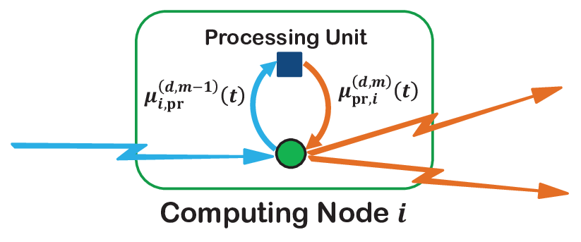
As is shown in Fig. 2, we represent the processing capabilities of wireless computing nodes via a processing element (e.g., CPU in a cloudlet node) co-located with each network node. A static, dedicated computing channel is considered, where the achievable processing rate at node $i$ with the allocation of $k$ processing resource units is given by $R_{i,k}$ in operations per timeslot. We use $\mu_{i,\text{pr}}^{(d,m)}(t)$ to denote the flow rate (in information units per timeslot) of commodity $(d,m)$ ($0\leq m<M$) from node $i$ to its processing element at time $t$, and $\mu_{\text{pr},i}^{(d,m)}(t)$ to denote the flow rate of commodity $(d,m)$ ($0<m\leq M$) from the processing element back to node $i$ (see Fig. 2). We then have the following MCC and maximum processing rate constraints:

Note that function $m$ at node $i$ processes input commodity $(d,m-1)$ at a rate $\mu_{i,\text{pr}}^{(d,m-1)}(t)$ information units per timeslot, using $\mu_{i,\text{pr}}^{(d,m-1)}(t)r^{(m)}$ operations per timeslot, and generates output commodity $(d,m)$ at a rate $\mu_{\text{pr},i}^{(d,m)}(t)$ information units per timeslot.

We assume that multiple transmitters (TXs) may transmit simultaneously to overlapping receivers (RXs) via the use of orthogonal broadcast channels of fixed bandwidth, a priori allocated by a given policy, whose design is outside the scope of this paper. On the other hand, due to the broadcast nature of the wireless medium, multiple RXs may overhear the transmission of a given TX. We model the channel between node $i$ and all other nodes in the network as a physically degraded Gaussian broadcast channel, where the network state process (the vector of all channel gains), denoted by ${\bf S}(t)\triangleq\{s_{ij}(t),\forall i,j\in\cal N\}$, evolves according to a Markov process with state space ${\mathcal{S}}$ and whose steady-state probability exists. We assume that the statistical CSI is known at the TX, while the instantaneous CSI can only be learned after the transmission has taken place and is thereby outdated (delayed).

It is well-known that superposition coding is optimal (capacity achieving) for the physically degraded broadcast channel with independent messages [15]. In particular, in this work we adopt the broadcast approach coding scheme (see [13, 14] and references therein), which consists of sending incremental information using superposition layers, such that the number of decoded layers at any RX depends on its own channel state, and the information decoded by a given RX is a subset of the information decoded by any other RX with no worse channel gain. That is, for a given transmitting node $i$, if we sort the $N-1$ potential receiving nodes in non-decreasing order of their channel gains $\{q_{i,1},\dots,q_{i,N-1}\}$, such that $q_{i,n}$ with $n\in\{1,\dots,N-1\}$ denotes the receiver with the $n$-th lowest channel gain, then the information decoded by receiver $q_{i,n}$ is also decoded by receiver $q_{i,u}$, for $u>n$. Moreover, let $\Omega_{i,n}\triangleq\{q_{i,n},\cdots,q_{i,N-1}\}$ be the set of receivers with the $N-n$ highest channel gains. Then, we can partition the information transmitted by node $i$ during a given timeslot into $N-1$ disjoint groups, with the $n$-th partition being the information whose successful receiver set is exactly $\Omega_{i,n}$, i.e., the information that is decoded by the nodes in $\Omega_{i,n}$, but not by the nodes in ${\mathcal{N}}\backslash\{i\}\backslash\{\Omega_{i,n}\}$. Fig. 3 illustrates the use of the broadcast approach for multi-receiver diversity.

Let ${p}_{i,k}(a)$ denote the optimal power density function over the continuum of superposition layers resulting from the allocation of $k$ transmission resource units at node $i$. Then, based on the broadcast approach [14], when allocating $k$ transmission resource units, the maximum achievable rate over link $(i,j)$ at time $t$ is given by

where $g_{ij}(t)$ is the channel gain over link $(i,j)$ at time $t$.

In practice, the continuum of superposition layers are discretized into a set of $L_{i},\forall i$, discrete code layers. In this case, the channel gain of each outgoing link from node $i$ at time $t$ can be discretized into $L_{i}+1$ states, denoted by $\mathcal{S}_{i}\triangleq\{\bar{s}_{i,0},\cdots,\bar{s}_{i,L_{i}}\}$, and $L_{i}$ channel gain thresholds $\{\bar{g}_{i,l},1\leq l\leq L_{i}:\bar{g}_{i,1}\leq\cdots\leq\bar{g}_{i,L_{i}}\}$. Then, we have

Let $P_{i,k}$ denote the total power associated with the allocation of $k$ transmission resource units at node $i$, and $P_{i,k}(l)$ the power allocated to code layer $l$, with $\sum_{l=1}^{L_{i}}P_{i,k}(l)=P_{i,k}$.²² 2 We assume that the power allocated to each layer is given and leave its optimization out of the scope the paper. We then use $\mathcal{R}_{i,k}\triangleq\{\bar{R}_{i,k}^{0},\cdots,\bar{R}_{i,k}^{L_{i}}\}$ to denote the maximum achievable transmission rates associated with the $L_{i}+1$ channel states, where

and $\bar{R}_{i,k}^{0}=0$.

Hence, the maximum achievable transmission rate over link $(i,j)$ at time $t$ is given by

The communication protocol between each TX-RX pair is illustrated in Fig. 4. At the beginning of each timeslot, TX and RX exchange all necessary control signals, including queue backlog state information (see Sec. II-F). Then, the TX decides how many transmission resource units to allocate for the given timeslot and how much rate to allocate to each available commodity. Afterwards, the transmission starts and lasts for a fixed time period (within the timeslot); during that time, both data and pilot tones (whose overhead is neglected) are transmitted.

After the transmission ends, every potential RX provides immediate feedback, containing the identification of the information decoded by the RX, which allows the TX to derive the experienced CSI. The TX then makes a forwarding decision and sends it through a final instruction to all the RXs, instructing each RX which portion of its decoded information to keep for further processing and/or forwarding (hence assigning the processing/forwarding responsibility). Control information, feedbacks, and final instructions are sent through a stable control channel, whose overhead is neglected.

We use $\mu_{ij}^{(d,m)}(t)$ to denote the amount of information of commodity $(d,m)$ retained by node $j$ after the transmission from node $i$ during timeslot $t$. In addition, it shall be useful to denote by $\mu_{iq_{i,u},n}^{(d,m)}(t)$ the information retained by node $q_{i,u}$ belonging to the $n$-th partition of node $i$’s transmitted information. Then, since $q_{i,u}\in\Omega_{i,n}$ for all $n$ satisfying $n\leq u$, we have

Moreover, according to the broadcast approach, the maximum achievable rate of the $n$-th partition, given the allocation of $k$ transmission resource units at time $t$, is $R_{i{q_{i,n}},k}(t)-R_{i{q_{i,n-1}},k}(t)$. We then have,

where $R_{iq_{i,0},k}\!\left(t\right)=0$, for all $i,k,t$.

Note that Eqs. (5) and (6) lead to the following rate constraint on link $(i,j)$ for all $t$: $\sum\nolimits_{(d,m)}\mu_{ij}^{\left({d,m}\right)}\!\left(t\right)\leq\sum\nolimits_{k=0}^{K_{i}^{\text{tr}}}R_{ij,k}(t)\ y_{i,k}^{\text{tr}}(t)$.

We denote by $a_{i}^{(d,m)}(t)$ the exogenous arrival rate of commodity $(d,m)$ at node $i$ at time $t$, and by $\lambda_{i}^{(d,m)}$ its expected value. We assume that $a_{i}^{(d,m)}(t)$ is independently and identically distributed (i.i.d.) across timeslots and its forth moment is upper bounded,³³ 3 The upper bound of the fourth moment is used in the proof of convergence with probability $1$ in Theorem 2. i.e., $\mathbb{E}\{(\sum_{(d,m)}{a_{i}^{(d,m)}(t)})^{4}\}\leq A_{\max}^{4}$. Recall that in an AgI service only the source commodity $(d,0)$ enters the network exogenously, while all other commodities are created inside the network as the output of a service function. Hence, $a_{i}^{(d,m)}(t)=0$, for all $i,t$ when $m>0$.

During AgI service delivery, internal network queues buffer incoming data according to their commodities. We define the queue backlog of commodity $(d,m)$ at node $i$, $Q_{i}^{(d,m)}(t)$, as the amount (in information units) of commodity $(d,m)$ in the queue of node $i$ at the beginning of timeslot $t$, which evolves over time as follows:

Note that in an AgI service only the final commodity $(d,M)$ is allowed to exit the network once it arrives to its destination $d\in\cal D$, while any other commodity $(d,m)$, $m<M$, can only get consumed by being processed into the next commodity $(d,m+1)$ of the service chain. Final commodity $(d,M)$ is assumed to leave the network immediately upon arrival/decoding at its destination, i.e., $Q_{d}^{(d,M)}(t)=0$, for all $d,t$.

The goal is to design a control algorithm that dynamically schedules, routes, and process service flows over the wireless computing network with minimum total average resource cost,

where $h(t)$ is the total cost of the network at time $t$,

while ensuring that the network is rate stable [10], i.e.,

Dynamic Wireless Computing Network Control (DWCNC):

Local processing decisions: At the beginning of timeslot $t$, each node $i$ observes its local queue backlogs and performs the following operations:

1. 1.

   Compute the processing utility weight of each commodity $(d,m)$:

   $\displaystyle W_{i}^{(d,m)}(t)\!\mathrel{\mathop{\kern 0.0pt=}\limits^{\Delta}}\!\frac{1}{r^{(m+1)}}\!\left[Q_{i}^{(d,m)}(t)\!-\!\xi^{(m\scalebox{0.7}{$+1$})}Q_{i}^{(d,m\scalebox{0.7}{$+1$})}(t)\right]^{\!+},$

   where we denote $[x]^{+}=\max\{x,0\}$. Note that $W_{i}^{(d,m)}(t)$ indicates the “potential benefit” of executing function $(m\!+\!1)$ to process commodity $(d,m)$ into commodity $(d,m\!+\!1)$ at time $t$, in terms of local congestion reduction per processing operation.

2. 2.

   Compute the optimal number of processing resource units $k_{\text{pr}}^{\dagger}$ to allocate and the optimal commodity $(d,m)_{\text{pr}}^{{\dagger}}$ to process:

   $$\left[{k_{\text{pr}}^{\dagger},(d,m)_{\text{pr}}^{\dagger}}\right]\!=\!\mathop{\arg\max}\limits_{k,\left({d,m}\right)}\left\{{{R_{i,k}}W_{i}^{(d,m)}\!(t)-Vw_{i,k}^{\text{pr}}}\right\},$$

   (21)

   where $V$ is a non-negative control parameter that determines the degree to which cost is emphasized.

3. 3.

   Make the following flow rate assignment decisions:

   		$\displaystyle\mu_{i,\text{pr}}^{(d,m)_{\text{pr}}^{\dagger}}(t)={{{R_{i,{k_{\text{pr}}^{\dagger}}}}}\mathord{\left/{\vphantom{{{R_{i,{k^{\dagger}}}}}{{r^{(m+1)}}}}}\right.\kern-1.2pt}{{r^{(m^{\dagger}_{\text{pr}}+1)}}}};$
   		$\displaystyle\mu_{i,\text{pr}}^{(d,m)}(t)=0,\quad\forall(d,m)\neq(d,m)_{\text{pr}}^{\dagger}.$

Local wireless transmission decisions: At the beginning of timeslot $t$, each node $i$ observes its local queue backlogs, the queue backlogs of its potential RXs and the associated statistical CSI, and performs the following operations:

1. 1.

   For each outgoing link $(i,j)$, compute the differential backlog weight of each commodity $(d,m)$:

   $$W_{ij}^{(d,m)}(t)\triangleq\left[Q_{i}^{(d,m)}(t)-Q_{j}^{(d,m)}(t)\right]^{+}.$$

2. 2.

   For each transmission resource allocation choice $k\in\{0,\dots,K_{i}^{\text{tr}}\}$, compute the transmission utility weight of each commodity $(d,m)$:

   $\displaystyle\scalebox{0.95}{$W_{i,k,\text{tr}}^{(d,m)}\left(t\right)\triangleq\sum\limits_{{\bf{s}}\in S}{\Pr\left({\left.{{\bf{S}}(t)={\bf{s}}}\right|{\bf{S}}\left({t-1}\right)}=\tilde{\bf{s}}\right)}\sum\limits_{n=1}^{N-1}\!\!{\left[{{R_{i{q_{i,n}},k}}\left({\bf{s}}\right)-{R_{i{q_{i,n-1}},k}}\left({\bf{s}}\right)}\right]\!\mathop{\max}\limits_{j\in{\Omega_{i,n}}\left({\bf{s}}\right)}\!\left\{{W_{ij}^{(d,m)}\!\left(t\right)}\!\right\}}$},$

   (22)

   where $\tilde{\bf{s}}$ denotes the CSI feedbacks at time $t-1$, and, with an abuse of notation, ${\Omega_{i,n}}({\bf{s}})$ is used to indicate the dependence of ${\Omega_{i,n}}$ on the network state $\bf s$.

3. 3.

   Compute the optimal number of transmission resource units $k_{\text{tr}}^{{\dagger}}$ to allocate and the optimal commodity $(d,m)_{\text{tr}}^{{\dagger}}$ to transmit:

   $$\left[{{k_{\text{tr}}^{{\dagger}}},{{\left({d,m}\right)}_{\text{tr}}^{{\dagger}}}}\right]=\mathop{\arg\max}\limits_{k,\left({d,m}\right)}\left\{{W_{i,k,\text{tr}}^{(d,m)}\left(t\right)}-Vw_{i,k}^{\text{tr}}\right\}.$$

   (23)

   If $k_{\text{tr}}^{{\dagger}}=0$, node $i$ keeps silent in timeslot $t$.

4. 4.

   After receiving the CSI feedbacks, node $i$ identifies the information decoded by each RX and assigns the processing/forwarding responsibility for the $n$-th partition of the transmitted information to the RX in $\Omega_{i,n}({\bf S}(t))$ with the largest positive $W_{ij}^{(d,m)}(t)$, while all other RXs in $\Omega_{i,n}({\bf S}(t))$ and node $i$ discard the information. If no receiver in $\Omega_{i,n}({\bf S}(t))$ has positive $W_{ij}^{(d,m)}(t)$, node $i$ retains the information of partition $n$, while all the receivers in $\Omega_{i,n}({\bf S}(t))$ discard it.

Remarks:

• •

  In the local processing decisions, maximizing the metric in (21) over $[k,(d,m)]$ can be decomposed into first maximizing $W_{i}^{(d,m)}(t)$ over $(d,m)$ and then maximizing the metric over $k$ given the maximized $W_{i}^{(d,m)}(t)$. The computational complexity is $O(K_{i}^{\text{pr}}+NM)$.

• •

  In Step 2 of the local transmission decisions, $W_{i,k,\text{tr}}^{(d,m)}(t)$ is computed according to (22) using the transition probabilities $\Pr(\left.{\bf S}(t)={\bf s}\right|{\bf S}(t-1)=\tilde{\bf s})$, known as the statistical CSI, but the complexity can be high due to the possibly exponentially large network state space with respect to the number of links. However, the computation can be significantly simplified when the channel realizations of the wireless links are mutually independent, which is described in the next subsection.

• •

  The fact of discarding decoded information at the RXs that do not get the processing/forwarding responsibility during Step 4 of the local transmission decisions, implies that DWCNC is a single-copy routing algorithm.

Recall that, in practice, when using the broadcast approach, each node uses a $L_{i}$ discrete code layers, with $R_{ij,k}(t)$ taking values in $R_{i,k}$ as described in Sec. II-D).

Let $\bar{\Omega}_{i,l}({\bf S}(t))$ denote the set of receivers that have channel gain no smaller than $\bar{g}_{i,l}$ at time $t$, i.e., $g_{ij}(t)\geq\bar{g}_{i,l}$ for all $j\in\bar{\Omega}_{i,l}({\bf S}(t))$, and $g_{ij}(t)<\bar{g}_{i,l}$ for all $j\notin\bar{\Omega}_{i,l}({\bf S}(t))$.

Given ${\bf S}(t)=\bf s$ and $k$, we have the following two possible cases for the maximum achievable transmission rate of the $n$-th partition: i) ${R_{i{q_{i,n}},k}}\left({\bf{s}}\right)-{R_{i{q_{i,n-1}},k}}\left({\bf{s}}\right)=0$; ii) ${R_{i{q_{i,n}},k}}\left({\bf{s}}\right)-{R_{i{q_{i,n-1}},k}}\left({\bf{s}}\right)=\sum\nolimits_{l=l_{0}}^{l_{1}}{\left({\bar{R}_{i,k}^{l}-\bar{R}_{i,k}^{l-1}}\right)}$, for some $l_{0}$ and $l_{1}$ satisfying $1\leq l_{0}\leq l_{1}\leq L_{i}$, with ${{\bar{\Omega}}_{i,l}}({\bf{s}})={\Omega_{i,n}}({\bf{s}})$ for $l_{0}\leq l\leq l_{1}$. Then we have, for all $i$, ${\bf s}$, $k$, $(d,m)$, and $t$,

based on which we can rewrite Eq. (22) as follows:

where $\mathcal{H}(t)\triangleq\{{\bf Q}(t),{\bf S}(t-1)\}$ is the ensemble of queue backlog observations at time $t$ and the CSI feedbacks at time $t-1$.

Let $1_{ij,l}^{(d,m)}(t)$ denote the indicator that takes value $1$ if receiver $j$ has the largest differential backlog $W_{ij}^{(d,m)}(t)$ among the receivers in $\bar{\Omega}_{i,l}({\bf S}(t))$, and $0$ otherwise. Then, we have

where $\varphi_{ij,l}^{\left({d,m}\right)}\left({\mathcal{H}(t)}\right)$ is the conditional probability that $1_{ij,l}^{(d,m)}(t)$ takes value $1$ given $\mathcal{H}(t)$.

Plugging (25) into (24) to compute $W_{i,k,\text{tr}}^{(d,m)}\left(t\right)$, we can replace Step 2 of the local transmission decisions of DWCNC in Sec. IV-A with the following two sub-steps:

1. 2a)

   For each commodity $(d,m)$, sort the receivers of node $i$ according to their differential backlog weight $W_{ij}^{(d,m)}(t)$ in non-increasing order. Let $\Psi_{ij}^{(d,m)}(t)$ denote the set of receivers of node $i$ with index smaller than the index of receiver $j$ in the sorted list at time $t$. In this case, each receiver in $\Psi_{ij}^{(d,m)}(t)$ has no smaller differential backlog weight than receiver $j$.

2. 2b)

   For each transmission resource allocation choice $k\in\{0,\dots,K_{i}^{\text{tr}}\}$, compute the transmission utility weight of each commodity $(d,m)$:

   $$W_{i,k,\text{tr}}^{(d,m)}\left(t\right)=\sum\nolimits_{l=1}^{{L_{i}}}{\left({\bar{R}_{i,k}^{l}-\bar{R}_{i,k}^{l-1}}\right)\sum\nolimits_{j}{W_{ij}^{(d,m)}\left(t\right)\varphi_{ij,l}^{\left({d,m}\right)}\left({\mathcal{H}(t)}\right)}}.$$

   (26)

Computing $\varphi_{ij,l}^{\left({d,m}\right)}\left({\mathcal{H}(t)}\right)$, which requires the statistical CSI, can be significantly simplified if the channel realizations of the links are mutually independent. In this case, the value of $\varphi_{ij,l}^{\left({d,m}\right)}\left({\mathcal{H}(t)}\right)$ can be obtained from a simple multiplication as follows:

References

• [1] H. Feng, J. Llorca, A. M. Tulino, A. F. Molisch, “On the delivery of augmented information services over wireless computing networks,” IEEE International Conference on Communications (ICC), Paris, June 2017, pp. 1-7.
• [2] Marcus Weldon, “The Future X Network,” CRC Press, October 2015.
• [3] L. Lewin-Eytan, J. Naor, R. Cohen, D. Raz, “Near Optimal Placement of Virtual Network Functions,” IEEE INFOCOM, 2015.
• [4] M. Barcelo, J. Llorca, A. M. Tulino, N. Raman, “The Cloud Servide Distribution Problem in Distributed Cloud Networks,” IEEE ICC, Sept. 2015.
• [5] H. Feng, J. Llorca, A. M. Tulino, D. Raz, A. F. Molisch, “Approximation Algorithms for the Network Service Distribution Problem,” IEEE INFOCOM, June 2017.
• [6] H. Feng, J. Llorca, A. M. Tulino, A. F. Molisch, “Dynamic Network Service Optimization in Distributed Cloud Networks,” IEEE INFOCOM SWFAN Workshop, Sept. 2016.
• [7] H. Feng, J. Llorca, A. M. Tulino and A. F. Molisch, “Optimal Dynamic Cloud Network Control,” IEEE ICC, Sept. 2016.
• [8] M. Chiang and T. Zhang, “Fog and IoT: An Overview of Research Opportunities”, IEEE Internet of Things Journal, vol. 3, no. 6, pp. 854-864, Dec. 2016.
• [9] M. Satyanarayanan, P. Bahl, R. Caceres and N. Davies, “The Case for VM-Based Cloudlets in Mobile Computing”, IEEE Pervasive Computing, vol. 8, no. 4, pp. 14-23, Oct.-Dec. 2009.
• [10] M. J. Neely, “Stochastic Network Optimization with Application to Communication and Queueing Systems”, Synthesis Lectures on Communication Networks, Morgan & Claypool, 2010.
• [11] M. J. Neely, “Optimal Backpressure Routing for Wireless Networks with Multi-Receiver Diversity”, Ad Hoc Networks, vol. 7, pp. 862–881, July 2009.
• [12] H. Feng and A. F. Molisch, “Diversity Backpressure Scheduling and Routing with Mutual Information Accumulation in Wireless Ad-hoc Networks”, IEEE Transactions on Information Theory, vol. 62, no. 12: pp. 7299-7323, Dec. 2016.
• [13] S. Shamai and A. Steiner. “A Broadcast Approach for A Single-user Slowly Fading MIMO Channel.” IEEE Transactions on Information Theory, vol. 49, no. 10: pp. 2617-2635, Oct. 2003.
• [14] A. M. Tulino, G. Caire and S. Shamai. “The Broadcast Approach for The Sparse-input Random-sampled MIMO Gaussian Channel,” IEEE ISIT, Aug. 2014.
• [15] A. El Gamal and Y.-H. Kim, “Network Information Theory,” Cambridge University Press, 2011.
• [16] A. F. Molisch, “Wireless communications,” 2nd ed., John Wiley &\& Sons, 2012.
• [17] M. J. Neely, “Queue Stability and Probability 11 Convergence via Lyapunov Optimization,” arXiv preprint:1008.3519, 2010.