Allocating and splitting free energy to maximize molecular machine flux
Abstract
Biomolecular machines transduce between different forms of energy. These machines make directed progress and increase their speed by consuming free energy, typically in the form of nonequilibrium chemical concentrations. Machine dynamics are often modeled by transitions between a set of discrete metastable conformational states. In general, the free energy change associated with each transition can increase the forward rate constant, decrease the reverse rate constant, or both. In contrast to previous optimizations, we find that in general flux is neither maximized by devoting all free energy changes to increasing forward rate constants nor by solely decreasing reverse rate constants. Instead the optimal free energy splitting depends on the detailed dynamics. Extending our analysis to machines with vulnerable states (from which they can break down), in the strong driving corresponding to in vivo cellular conditions, processivity is maximized by reducing the occupation of the vulnerable state.
1 Introduction
Molecular machines such as kinesin Clancy et al. (2011), helicase Caruthers and McKay (2002), and ubiquitin ligase Cardozo and Pagano (2004) perform diverse tasks inside cells. These machines typically convert nonequilibrium chemical concentrations, maintained by other machinery in the cell Boyer (1997); Fernie et al. (2004), into directed motion or work Vale and Milligan (2000); Bustamante et al. (2001). These microscopic machines operate stochastically Astumian and Bier (1994), with their fluctuating progress now experimentally observable with improving resolution (see e.g. Isojima et al Isojima et al. (2016)).
Quantitative models of molecular machines are pervasive, e.g. to investigate forces Fisher and Kolomeisky (1999), efficiency Schmiedl and Seifert (2008), and performance of different driving mechanisms Wagoner and Dill (2016); Astumian (2015). Each model usually treats molecular machine dynamics as a set of transitions between discrete metastable states Thomas et al. (2001), as diffusion on a continuous energy landscape Astumian et al. (2016), or a combination of the two Xing et al. (2005).
In this paper we study how the flux of cyclic machines, a posited driver of evolutionary fitness Nguyen et al. (2017), is affected by the details of free energy changes over a set of discrete states.
Earlier models considered how the influence of a load is quantitatively split between forward and reverse transitions Wagoner and Dill (2016); Schmiedl and Seifert (2008); Thomas et al. (2001); Fisher and Kolomeisky (1999). In this work we find that by extending the splitting to all free energy components, not just loads, there is no single splitting scheme that always maximizes the flux. Additionally, optimizing the allocation of a single free energy component compensates for any sub-optimal fixed allocations of other free energy components.
We also examine how to maximize progress for transiently processive cyclic machines with vulnerable states, from which the machine can break down or ‘escape’ (e.g. kinesin can dissociate from a microtubule Milic et al. (2014)). For strong driving, free energy is simply allocated to reduce the occupation of the state vulnerable to escape. However, under specific conditions, the optimal allocation is reversed, counterintuitively increasing processivity by increasing occupation of the vulnerable state.
2 Model
2.1 Discrete states
We consider cycles with two or three states (Fig. 1), often used for models of molecular motors or other driven systems inside living cells Kolomeisky and Fisher (2003); Qian (2006). For our model cycles, each forward rate constant describes transitions from state to state , with a corresponding reverse rate constant for transitions from state to state . To preserve microscopic reversibility Astumian (2015); Fisher and Kolomeisky (1999), any transition with a nonzero forward rate cannot be irreversible, and must also have a nonzero reverse rate.

Forward transitions from state to state occur at rate , for probability in state . Reverse transitions from state to state occur at reverse rate . (The two-state cycle has two pathways, 12 and 21, each with a forward and reverse direction, and each representing distinguishable physical transition mechanisms.)
To preferentially drive such cycles in a particular direction, cells use nonequilibrium concentrations of reacting chemical species, such as adenosine triphosphate (ATP), adenosine diphosphate (ADP), and inorganic phosphate () Phillips et al. (2012). ATP hydrolysis into ADP and yields a free energy that depends on the respective concentrations Phillips et al. (2012),
| (1) |
Here , is Boltzmann’s constant, and is the temperature of the thermal bath exchanging heat with the system. ATP hydrolysis provides free energy under typical physiological conditions Phillips et al. (2012). From here on we set , thus measuring all free energies in units of the thermal energy scale .
The free energy allocation of a given transition path fixes the ratio between the forward and reverse rate constants Wagoner and Dill (2016); Pietzonka et al. (2016); Rao and Esposito (2016),
| (2) |
Without to provide a bias, the full forward and reverse rate constants each equal the ‘bare’ rate constants . , where is the free energy change of the machine and its surroundings over the transition. over a given cycle must be negative to drive net progress in the forward direction (on average).
2.2 Biasing rates with free energy
can be composed of several different free energy components, including but not limited to conformational changes, binding/unbinding, or a change in potential.
The free energy change of the molecular machine over a transition includes free energy differences between distinct machine conformations, as well as changes in the free energy of any molecules bound to the machine (e.g. hydrolysis of ATP to ADP and ), as the free energy changes of the machine and bound species cannot be separated Hill and Eisenberg (1981); Hill (1983).
is the free energy change of the solution when a molecule binds the machine, leaving the solution, with the chemical potential of the molecule given the concentration in solution. includes molecules typically considered ‘fuel’, such as ATP; and those typically considered cargo. For a molecule that unbinds from the machine and joins the solution, .
represents the free energy change of the machine, or any object attached to the machine, due to an external potential or gradient, e.g. due to a bead attached to kinesin that is also in an optical trap.
We confine our attention in this paper to ‘reversible’ free energy components, whereby any free energy expended in a forward reaction is recovered by the reverse reaction. Thus we exclude from consideration any omnidirectional free energy dissipation, such as that due to friction when pulling a load through a viscous medium.
Excepting , we expect that the free energy components are relatively fixed (i.e. unable to be changed by a modification to the machine). , as the machine returns to the same state after completing each cycle – abiding by this constraint, variation of (nominally through machine mutations) can be used to optimize machine operation.
We model each free energy component with a different splitting factor Schmiedl and Seifert (2008); Wagoner and Dill (2016) , which describes how the effect of is divided between forward and reverse rate constants,
| (3) |
Earlier studies Wagoner and Dill (2016); Schmiedl and Seifert (2008); Thomas et al. (2001); Fisher and Kolomeisky (1999) considered a molecular motor pulling against a constant opposing force , with each cycle of the motor stepping forward a distance . The transition completing the step transduces free energy to the motor’s position in the potential. In our framework this corresponds to . For steps against this constant force, is known as a power stroke (PS) and is known as a Brownian ratchet (BR) Wagoner and Dill (2016).
In this paper we primarily consider the case where splitting factors have the same value for all free energy components. This simple framework assumes the transition state is similarly arrayed between the reactant and product along different coordinate axes. We label as forward labile (FL) and as reverse labile (RL). FL is then similar to BR, and RL to PS Brown and Sivak (2017). The choice between PS and BR, or between FL and RL, affects machine performance characteristics Wagoner and Dill (2016); Brown and Sivak (2017), and below we determine how to vary splitting factors to maximize flux.
3 Maximizing flux
3.1 Optimal splitting factors
Setting all splitting factors to the same value allows the combination of all terms in Eqs. 3 into single terms and , giving rate constants
| (4a) | ||||
| (4b) | ||||
We consider a two-state cycle, with steady-state flux (hereafter simply flux) Hill (1977)
| (5) |
Inserting Eq. 4 into Eq. 5 and differentiating with respect to gives
The cycle proceeds forward when . for all when both and ; for these conditions, (FL) maximizes the flux. For (RL) to maximize the flux requires
| (12) |
a more complicated condition to fulfill, as and cannot be simultaneously fulfilled with . Flux can also be maximized for intermediate , with changing sign (maximizing flux) when
| (13) |
The flux-maximizing value of splitting factor thus depends on free energy allocation and bare rate constants .
Although here we set , in Supplemental Information (SI): Varying splitting factors, we consider splitting factors that vary across different free energy components and different transitions. Notably, for splitting factors specific to each free energy component and transition , if then maximizes the flux, and if then maximizes the flux.
For a molecular motor pulling against a constant force, a forward step has free energy component . For independent variation of , flux is maximized for . In this scenario, the optimal splitting factor agrees with Wagoner and Dill’s finding that maximizes the power Wagoner and Dill (2016). Our results are generally distinct, and do not find a universal optimal value, because we generalize to cycles with multiple states and splitting factors that apply to all free energy components, not just the free energy component associated with pulling against a constant force.
Fig. 2 shows the variation in flux as the splitting factor is varied from the flux-maximizing value in the range . The flux can be maximized at an extreme splitting factor value, (left panels) or (not shown, but possible), or between the extreme values, (right panels). The flux can decrease by more than an order of magnitude away from the optimal value, and decreases faster for larger .
 |
3.2 Optimal free energy allocation
Considering Eq. 4, we vary the free energy allocated to each transition to adjust the rate constants and maximize the flux.
For the total free energy budget per cycle , the flux-maximizing free energy allocation satisfies (see SI: Varying free energy)
| (14) | ||||
This cannot generally be solved for .
For equal splitting factors , rate constants are determined by the sum of all free energy components , such that if all but one free energy component is fixed, the remaining free energy component can be varied to achieve any desired sum. This makes maximal flux attainable by only adjusting the free energy allocation of the molecular machine, .
For and the rate constants reduce to those of our previous work Brown and Sivak (2017), from which the flux-maximizing free energy allocation can be determined. For (FL),
| (15) |
For (RL),
| (16) |
may be decomposed into multiple free energy components; for conceptual clarity we limit our discussion to two, , but our results trivially generalize. With , , and , then for , Eq. 15 becomes
| (17) |
If one component is fixed (without loss of generality ), then can vary to preserve the flux-maximizing allocation . Effectively, the variable component of can compensate for the fixed component to maximize the flux.
In earlier work Brown and Sivak (2017), we showed that for a range of several around the optimal allocation, the flux can decrease by more than an order of magnitude. The free energy allocation can thus meaningfully alter the cycle output.
In this section we considered equal splitting factors for all free energy components and transitions: . In SI: Varying free energy, we consider the more general case where the splitting factor varies over free energy components and transitions, similarly finding that variable free energy components compensate for fixed components.
3.3 Robustness to variable load
The in vivo operating environment of molecular machines is diverse, with variable cargo, molecular concentrations, and other factors causing some free energy components to vary over the life-cycle of a machine. We consider a scenario with two free energy components over a cycle, and . has some fixed value, but is a load that can be applied or removed, with (no load) or (load). The allocation of to the various is fixed. If the allocation of is optimized without (with) an applied load, but then the load is applied (removed), the flux will generally be lower than if is optimized under the correct conditions. Fig. 3 shows the flux as a function of load for (that of ATP at physiological conditions) for the four possible scenarios, optimized with () or without load () and subsequently applying or not applying a load.
 |
The fluxes for the four scenarios have a fixed order, independent of model parameters. Without load, cycle flux is higher under the correctly optimized allocation than under incorrectly optimized for load; under the flux is higher without load than with, because adding a resistive load always reduces the flux; and with load, flux under the correctly optimized is higher than under the incorrectly optimized . Due to this fixed ordering, the flux changes less when the load is applied or removed if the free energy component allocation is optimized with a load (), compared to if the allocation is optimized for no load ().
4 Processivity
Many cycles are transiently processive, eventually ‘escaping’ from their processive mode of operation, precluding further progress. For example, a transport motor can detach from its cytoskeletal track and diffuse away, effectively ending its forward transport Milic et al. (2014); Hodges et al. (2007).
We model escape from a single ‘vulnerable’ state (without loss of generality, state 2), consistent with experiments suggesting kinesin primarily detaches from a subset of states Milic et al. (2014); Andreasson et al. (2015); Muthukrishnan et al. (2015); Nam and Epureanu (2015); Topraka et al. (2009). The vulnerable state has an escape rate constant . The states which are not vulnerable have the same dynamics as earlier. For the two-state cycle, escape produces modified state 2 dynamics
| (18) |
For , probability leaves the cycle and there are no steady states for occupation probabilities (except ). Instead, we find steady states for the fractional probabilities (see SI: Processivity), for total remaining probability . This determines the dynamics of , and thus the average fluxes in the cycle at all times : .
Unlike a cycle without escape, in the steady state of the fluxes for the different transitions will not generally be equal. For the two-state cycle, the changes in probabilities are determined by the flux into and out of the respective states:
| (19a) | ||||
| (19b) | ||||
Once reaches steady state, . Substituting this into Eqs. 19 and rearranging gives the pathway (or one-sided) steady-state flux
| (20) |
4.1 Accumulated flux
Because the flux decays with time as probability escapes, we additionally include the rate of escape in our evaluation of molecular machine progress. Instead of flux alone, we combine flux and (avoided) escape into the ‘accumulated flux’,
| (21) |
For , can always be increased by adjusting to reduce and thus reduce escape, so has no maximum, hence we maximize after a finite time .
For simplicity, we consider two-state cycles with a single splitting factor . We set bare rate constants , such that all escape rate constants are in units of this bare rate. Fig. 4 shows two-state free energy allocations that maximize accumulated flux for FL and RL schemes at various finite times , for two distinct escape rate constants (see SI: Processivity for similar three-state results). These escape rate constants are consistent with modeling that suggests the detachment timescale from the vulnerable state of myosin V is 10-1000 slower than other timescales in the main forward pathway at zero force Hinczewski et al. (2013).
 |
A prominent feature of Fig. 4 is the approximate collapse of cycles with different to the same (where ), demonstrating that the optimal free energy allocation for the parameter values shown in Fig. 4 (SI: Processivity shows optimal allocations for larger , which do not collapse). For FL cycles with small and ,
| (22) |
and for RL,
| (23) |
See SI: Processivity for derivations. In Fig. 4, Eqs. 22 and 23 (thick black dotted curves) closely match the numerical (solid and dashed curves) for low and low .
For high free energy budget , the allocation in Fig. 4 is intuitive: is low and (although not shown in the figure) is high, reducing the probability of being in the vulnerable state 2. For higher escape rates and longer times, the difference between optimal and naive allocations increases, diverging as time .
In Fig. 4, for FL changes sign from negative to positive as decreases, with the change occurring at larger for shorter times. Positive increases the probability in the vulnerable state and increases the escape rate. But maximizing is a tradeoff between reducing escape and increasing ongoing flux. For longer times and higher , it is more important to reduce escape to preserve the future flux, and the intuitive result () is observed. However, at small and , initial flux is relatively more important, as little escape occurs before time is reached. The escaping flux from state 2 causes for naive free energy allocation . FL only allows the forward fluxes to be increased — to maximize the flux, the forward flux for transition 12 should be increased more, because , leading to . In contrast, RL only allows reverse fluxes to be decreased — to maximize the flux, the reverse flux for transition 21 should be decreased more, again because , consistently leading to .
5 Discussion
Biomolecular machines perform a variety of tasks inside cells, driven by the free energy stored in intracellular chemical concentrations. Here we investigated how to maximize flux in molecular machines with multiple free energy components, and how to maintain processivity.
Central to our approach is the general manner in which forward and reverse rate constants are affected by free energy changes Brown and Sivak (2017); Schmiedl and Seifert (2008); Wagoner and Dill (2016). Free energy components that only affect the forward or reverse rate constants represent extremes, and the division of the effect of free energy components between the forward and reverse rate constants is more generally described by a splitting factor . We primarily consider the simplifying case where splitting factors for all distinct free energy components are equal.
In contrast with previous results Wagoner and Dill (2016), we find no single splitting factor generally maximizes the flux. Instead, the optimal splitting factor depends on the detailed free energy allocation, with flux decreasing significantly away from the optimal splitting factor (Fig. 2).
Previous studies Wagoner and Dill (2016); Schmiedl and Seifert (2008) argued that low splitting factors are optimal, suggesting low splitting factors would describe the operation of evolved biomolecular machines. We have shown that both low and high splitting factors can maximize flux, and that the optimal splitting factor value depends on the allocation of free energy. Experimental fits of splitting factors find both low splitting factors Zimmermann and Seifert (2012); Fisher and Kolomeisky (2001); Kolomeisky and Fisher (2003); Hwang and Hyeon (2017); Schmiedl and Seifert (2008) and high splitting factors Fisher and Kolomeisky (2001); Liepelt and Lipowsky (2007). These fits use several models for the dependence of rate constants on resisting forces Zimmermann and Seifert (2012); Fisher and Kolomeisky (2001); Lau et al. (2007); Kolomeisky and Fisher (2003); Hwang and Hyeon (2017); Schmiedl and Seifert (2008); Liepelt and Lipowsky (2007). Unlike in our model, all other models we have found assume that rate constants only explicitly contain splitting factors for force, with no splitting factors for other free energy components (though one other model has implicit splitting of the effect of chemical potential Schmiedl and Seifert (2008)). Splitting factor analysis has largely been done in the context of ‘canonical’ molecular machines, such as the walking motors kinesin Fisher and Kolomeisky (2001); Lau et al. (2007); Hwang and Hyeon (2017); Liepelt and Lipowsky (2007), myosin Kolomeisky and Fisher (2003); Schmiedl and Seifert (2008), and dynein Singh et al. (2005), or the rotary motor F1-ATPase Zimmermann and Seifert (2012). Splitting factors are not always robust, with distinct data sets for kinesin motility Visscher et al. (1999); Carter and Cross (2005) leading to substantially different inferred values of 0.3 and 0.65 Liepelt and Lipowsky (2007). It would be an interesting follow up to investigate splitting factors for all free energy components affecting rate constants, and for a broader class of molecular machines, which may lead to a broader diversity of splitting factor values. In SI: Experimental splitting factors, we describe in more detail the fitted splitting factors for various models Zimmermann and Seifert (2012); Fisher and Kolomeisky (2001); Lau et al. (2007); Kolomeisky and Fisher (2003); Hwang and Hyeon (2017); Schmiedl and Seifert (2008); Liepelt and Lipowsky (2007).
Flux can also be maximized by varying free energy components , with flux significantly decreasing away from the optimal . For a scenario with two distinct free energy components, one variable and one fixed, the flux is maximized by allocating the variable free energy component to compensate for any departure from optimal of the fixed free energy component allocation. There are examples of machine models fit to experimental data where transitions with a fixed load appear to receive more of the other free energy components than those without a load (consistent with our predictions) Fisher and Kolomeisky (2001); Clancy et al. (2011); Hwang and Hyeon (2017), but also counter-examples that do not fit this optimal framework Lau et al. (2007); Kolomeisky and Fisher (2003).
Through mutation, biomolecular machine operation can change, and we expect evolution to select machine parameters that favor certain performance characteristics. We argue that robustness increases when tuning parameters to maximize flux with a load, rather than without a load, because for load-optimized parameters the flux is less sensitive to the presence or absence of load. This is consistent with observations of kinesin maintaining a stable velocity under a range of forces Wang et al. (2017), an intuitively beneficial trait Mukherjee et al. (2017).
We also examined cycles that are transiently processive and escape from a single vulnerable state. For large free energy budgets, maximizing the number of complete cycles before the cycle escapes leads to intuitive allocations: free energy is primarily allocated to decrease the probability present in the vulnerable state. However, for small free energy budgets, to maximize the number of cycles completed, free energy is primarily allocated to increase the flux — for forward labile cycles this increases the probability present in the vulnerable state, while for reverse labile cycles this decreases it. Although this forward labile allocation increases the rate of escape, the associated flux increase more than compensates, leading to an overall increase in the accumulated flux.
Kinesins mutated to have different neck linker charge show increased processivity, which is attributed to shorter waiting times in states vulnerable to detachment from the microtubule Andreasson et al. (2015); Thorn et al. (2000); Topraka et al. (2009). These findings are consistent with our result that occupation of the vulnerable state be reduced to maximize processivity for large free energy budgets, such as the of free energy from ATP hydrolysis Phillips et al. (2012) driving each kinesin cycle Schnitzer and Block (1997).
While we are unaware of other modeling that maximizes processivity, Hill modeled escape as a transition to the initial state where all trajectories begin, effectively acting as an additional subcycle Hill (1988). This steady state with immediate rebinding is distinct from our steady state without rebinding. Both Hill’s approach and ours allow calculation of detachment rates (distinct due to differing steady states); but our approach additionally quantifies progress before detachment.
6 Supplemental Information
6.1 Maximizing flux: Varying splitting factors
Free energy components influence the forward and reverse rate constants, parameterized by ,
| (S1) |
In the main text we showed that if , there is no value of that generally maximizes the flux. The results of this section, with no consistent sign for , , and , similarly conclude that there are no generally optimal values for . Having no general optimal value does not align with previous results Wagoner and Dill (2016) where the power of a motor was maximized for a power stroke ().
The two-state cycle steady-state flux is
| (S2) |
For the cases below we consider two free energy components, and , subject to the relationships , , and .
6.1.1 Case 1
In this case, we allow the splitting constants to differ between transitions, but require equality for different free energy components, . This gives flux
| (S3) |
The flux increases with increasing as
| (S4) |
The flux is maximized for if and for if . Variation of produces a similar result.
6.1.2 Case 2
If we allow the splitting constants to differ for different free energy components, but not between transitions, so that and in Eq. S1, the flux and its derivative are
| (S5a) | ||||
| (S5b) | ||||
If and then , and maximizes the flux. However, both and are not always positive, so is not always positive or negative, with the flux maximized for
| (S6) |
Similar results are found for variation of .
6.1.3 Case 3
The most general case has splitting constants varying between transitions and between free energy components, as in Eq. S1, giving
| (S7a) | ||||
| (S7b) | ||||
If , then , leading to maximizing flux; conversely leads to maximizing flux. Similar results are found for variation of , , and .
6.2 Maximizing flux: Varying free energy
Here we examine what free energy allocation (composed of free energy components ) maximizes the flux. We go through distinct cases for splitting the effect of two free energy components between forward and reverse rate constants. In the main text, we find that for free energy components split identically across all transitions (), there is no closed form for the optimal free energy allocation , but that for or , closed forms can be found. We review these results below, as well as other splitting scenarios with similar results.
6.2.1 Case 1
Here both free energy components are split identically across all transitions, , giving rate constants
| (S8) |
The flux and its derivative are
| (S9a) | ||||
| (S9b) | ||||
Setting yields
| (S10) |
6.2.2 Case 2
For this case two free energy components are split differently, but the splitting is the same for all transitions. The rate constants are then
| (S11) |
The flux and its derivative are
| (S12a) | ||||
6.2.3 Case 3
For this case, different free energy components are split the same, but the splitting is different for each transition. The rate constants are then
| (S13) |
The flux and its derivative are
| (S14a) | ||||
6.2.4 Case 4
For this case, different free energy components are split differently, and the splitting is different for each transition. The rate constants are then
| (S15) |
The flux and its derivative are
| (S16a) | ||||
Case 1 is considered in the main text, while cases 2-4 are not. A closed form for (when splitting factors are equal for different free energy components) or (when they are not) solving or , respectively, cannot generally be found for any of these cases. We now consider some simplifying cases, with one or both of splitting factors and set to the extremes 0 or 1, to arrive at some closed-form solutions for .
6.2.5 Case 5
For this case, all free energy components split the same, and the splitting is the same for each transition, with splitting factor , corresponding to forward labile. Setting in Eq. S10 gives the flux-maximizing free energy allocation
| (S17) |
This corresponds to
| (S18) |
6.2.6 Case 6
For this case, all free energy components split the same, and the splitting is the same for each transition, with splitting factor corresponding to reverse labile. Setting in Eq. S10 gives the flux-maximizing free energy allocation
| (S19) |
This corresponds to
| (S20) |
For cases 5 and 6 the flux-maximizing allocation of compensates exactly for on each transition, and uses the remaining free energy to maximize the flux as if .
6.3 Experimental splitting factors
Table S1 summarizes splitting factors derived from fits to experimental data.
| range | Model | Machine |
|---|---|---|
| Eq. S21 | MyosinSchmiedl and Seifert (2008) | |
| Eq. S24 | MyosinKolomeisky and Fisher (2003) | |
| Eq. S24 | KinesinHwang and Hyeon (2017) | |
| Eq. S22 | F1 ATPaseZimmermann and Seifert (2012) | |
| Eq. S24 | Kinesin (four-state)Fisher and Kolomeisky (2001) | |
| Eq. S24 | Kinesin (two-state)Fisher and Kolomeisky (2001) | |
| Eq. S23 | KinesinLiepelt and Lipowsky (2007) | |
| Eq. S24 | KinesinLau et al. (2007) |
In Schmiedl and Seifert Schmiedl and Seifert (2008) a discrete-state model has rate constants
| (S21a) | ||||
| (S21b) | ||||
Their are identical to our splitting factors. For a two-state myosin model, they find and .
Zimmermann and Seifert Zimmermann and Seifert (2012) model a continuous free energy landscape with forward and reverse rate constants
| (S22a) | ||||
| (S22b) | ||||
is motor step size, is the spring constant between the motor and attached probe, and are the chemical potential differences from equilibrium. Rate constants and do not have indices because the model contains only one step. Splitting factor is found by fitting to experimental F1 ATPase data.
In Liepelt and Lipowsky Liepelt and Lipowsky (2007) a discrete-state model has rate constants
| (S23) |
For chemical transitions, , with a dimensionless force parameter similar to or . For mechanical transitions, for the direction against the load, and for the opposite direction. Using distinct kinesin motility data sets Visscher et al. (1999); Carter and Cross (2005), they find or 0.6.
Fisher and Kolomeisky Fisher and Kolomeisky (2001) construct a discrete-state model with forward and reverse rate constants
| (S24a) | ||||
| (S24b) | ||||
is a constant opposing force, is the motor step over a complete cycle, and are the rate constants at zero force. The are found by fitting to experimental kinesin data, but are not identical to our splitting factors . Instead, they use the constraint , such that is a combination of allocating a load to the various transitions and splitting the impact of the load between the forward and reverse rate constants. For a two-state model, for the first transition, they find and , equivalent to . For the second transition, they find and , equivalent to . For a four-state model, the first transition is found to have and (), the second transition and (), the third transition and (), and the fourth transition and (). The second transition of the two-state model, and the fourth transition of the four-state model, are treated as the most irreversible, indicating these transitions are allocated the most free energy. These transitions are also fit with the largest values, so that more of the other free energy components are allocated to transitions with more load. A later publication by the same authors Kolomeisky and Fisher (2003), with a two-state myosin model using the same force dependence, fitted the first transition with and () and a second transition with and (). In this case, the second transition is fit with a greater load, but is not allocated a greater amount of other free energy components.
In Hwang and Hyeon Hwang and Hyeon (2017), a discrete-state model for kinesin has forward and reverse rate constants with the same force dependence as Eq. S24. With four states, the first transition is fit with and (), the second transition with and (), the third transition with and (), and the fourth transition with and (). The second transition is fit with the largest load (high values) and has a larger amount of the other free energy components.
In Lau et al Lau et al. (2007), a discrete-state model for kinesin has forward and reverse rate constants with the same force dependence as Eq. S24. With two states, the first transition is fitted with and () and the second transition with and (). These are fit with the constraint . The transition state picture (e.g. in Schmiedl and Seifert Schmiedl and Seifert (2008)) describes an opposing force as reducing the rate of forward transitions and/or increasing the rate of reverse transitions. This transition state picture does not explain the values in Lau et al Lau et al. (2007) because for transition 12 both the forward and reverse transition rates are decreased by opposing force.
6.4 Processivity
6.4.1 Two states
With state 2 vulnerable to escape, the governing differential equations are
| (S25a) | ||||
| (S25b) | ||||
We rewrite these differential equations in terms of , where is the total remaining probability that has not yet escaped the cycle. Using
| (S26) |
and , gives
| (S27) |
Substituting into Eq. S27 at steady state (when ) gives a quadratic equation for :
| (S28) |
has a real solution when the discriminant is non-negative.
6.4.2 Optimizing two-state flux accumulated over large
Fig. 4 shows that for small and , changes monotonically as increases. However, for and , is non-monotonic (Fig. S1). As mentioned in the main text, the accumulated flux is the integrated flux over a period of time, and reflects both the instantaneous flux and escape from state 2. Increasing shifts the respective functional dependences of flux and on , often in ways producing competing influences on . For sufficiently high , the functional dependences asymptote to forms that don’t change with further increased . For small and , these functional dependences cease changing at approximately the same high value of , leading to be monotonic in in Fig. 4. However for larger and , the functional dependences cease changing at different values of . Since the (potentially countervailing) influences on do not happen over the same range, can change non-monotonically with , as seen for and in Fig. S1.
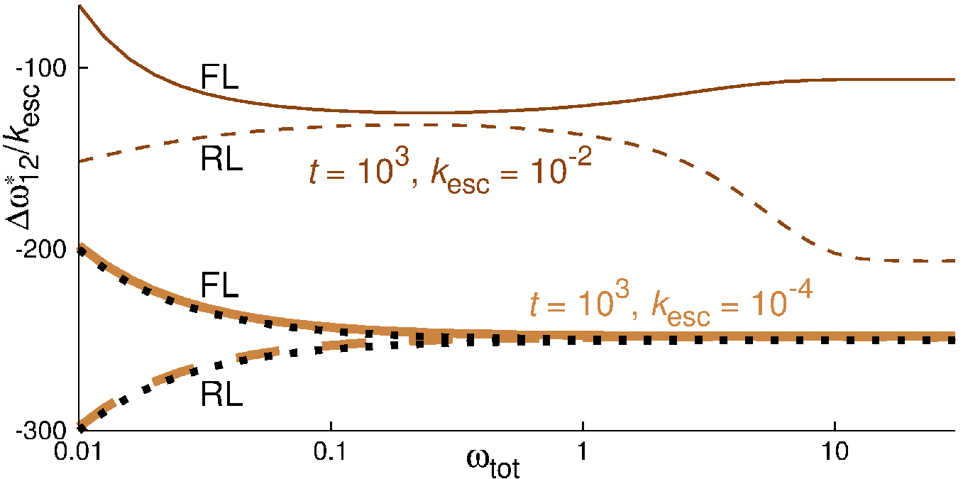 |
For and (Fig. S1), for FL and RL do not coincide at high . This distinction between FL and RL at high occurs because with more free energy dissipation, FL increases rate constants while RL decreases rate constants. At high , the rate constants for FL can still significantly change with more , while the rate constants for RL are already quite small. This leads RL to require a larger than FL. This effect also occurs for lower and in Fig. 4, but is much smaller because escape rates and/or total probability escaping is much smaller.
6.4.3 Two-state optimization approximation for low ,
Equations 17 and 18 are approximations for the free energy allocation that maximize the accumulated flux for small and .
We first derive Eq. 17 for FL rate constants with , , and , beginning with Eq. S28 and solving for using the quadratic formula,
| (S29) |
Taylor expanding for small and gives
| (S30) |
The flux is
| (S31) |
Inserting and from Eq. S30 into Eq. S31 and Taylor expanding for small gives
| (S32) |
We approximate the accumulated flux for as
| (S33a) | ||||
| (S33b) | ||||
with the second line dropping the for the . Inserting Eqs. S30 and S32, and their derivatives, into (using Eq. S33b for ), and dropping all terms of higher order than and , produces Eq. 17 (reproduced here for convenience),
| (S34) |
A similar derivation for RL rate constants leads to Eq. 18,
| (S35) |
We find the same equations using Maple 2016, keeping all non-Taylor expanded expressions, and then Taylor expanding the final derivative for small and .
For both FL and RL, escape is reduced by a more negative . Reducing escape grows in importance for longer times, hence the negative sign of the -dependent term in both Eqs. (S34) and (S35). For , escape causes at steady state, leading to be positive for FL (increasing the forward rate constant from the state with larger steady-state probability) and negative for RL (increasing the reverse rate constant from the state with larger steady-state probability). Hence the -independent term in is positive for FL (Eq. (S34)) and negative for RL (Eq. (S35)). With FL and for large , the forward rate constants are very large, so escape influences and negligibly at , so the -independent term of Eq. (S34) decreases in magnitude towards zero as increases. With RL and for large , the reverse rate constants are very small, so the influence of escape on and becomes insensitive to increases, so the -independent term of Eq. (S35) decreases in magnitude to a constant value as increases.
 |
 |
6.4.4 Three states
The three-state cycle with state 2 vulnerable to escape is governed by differential equations
| (S36a) | ||||
| (S36b) | ||||
| (S36c) | ||||
Setting gives
| (S38a) | ||||
| (S38b) | ||||
| (S38c) | ||||
Substituting these equations into Eq. S37b produces a cubic equation for ,
| (S39) | ||||
Cubic equations generally have at least one real solution, so a real exists.
Solving the cubic for in Eq. S39 determines the steady-state and . Because the flux decays with time as probability escapes, we additionally consider the rate of escape to evaluate molecular machine progress. Instead of flux alone, we combine flux and escape into the accumulated flux
| (S40) |
which we maximize after a time . Figs. S2 (FL cycles) and S3 (RL cycles) show allocations which maximize . These three-state results are similar to the two-state results in the main text.
References
- Clancy et al. (2011) Clancy, B. E.; Behnke-Parks, W. M.; Andreasson, J. O. L.; Rosenfeld, S. S.; Block, S. M. Pathway for kinesin stepping. Nat. Struct. Mol. Biol. 2011, 18, 1020–1027.
- Caruthers and McKay (2002) Caruthers, J. M.; McKay, D. B. Helicase structure and mechanism. Curr. Opin. Struct. Biol. 2002, 12, 123–133.
- Cardozo and Pagano (2004) Cardozo, T.; Pagano, M. The SCF ubiquitin ligase: insights into a molecular machine. Nat. Rev. Mol. Cell Biol. 2004, 5, 739–751.
- Boyer (1997) Boyer, P. D. The ATP synthase — a splendid molecular machine. Annu. Rev. Biochem. 1997, 66, 717–749.
- Fernie et al. (2004) Fernie, A. R.; Carrari, F.; Sweetlove, L. J. Respiratory metabolism: glycolysis, the TCA cycle and mitochondrial electron transport. Curr. Opin. Plant Biol. 2004, 7, 254–261.
- Vale and Milligan (2000) Vale, R. D.; Milligan, R. A. The way things move: looking under the hood of molecular motor proteins. Science 2000, 288, 88–95.
- Bustamante et al. (2001) Bustamante, C.; Keller, D.; Oster, G. The physics of molecular motors. Acc. Chem. Res. 2001, 34, 412–420.
- Astumian and Bier (1994) Astumian, R. D.; Bier, M. Fluctuation driven ratchets: molecular motors. Phys. Rev. Lett. 1994, 72, 1766–1769.
- Isojima et al. (2016) Isojima, H.; Iino, R.; Niitani, Y.; Noji, H.; Tomishige, M. Direct observation of intermediate states during the stepping motion of kinesin-1. Nat. Chem. Biol. 2016, 12, 290–297.
- Fisher and Kolomeisky (1999) Fisher, M. E.; Kolomeisky, A. B. The force exerted by a molecular motor. Proc. Natl. Acad. Sci. USA 1999, 96, 6597–6602.
- Schmiedl and Seifert (2008) Schmiedl, T.; Seifert, U. Efficiency of molecular motors at maximum power. Europhys. Lett. 2008, 83, 30005.
- Wagoner and Dill (2016) Wagoner, J. A.; Dill, K. A. Molecular motors: power strokes outperform Brownian ratchets. J. Phys. Chem. B 2016, 120, 6327–6336.
- Astumian (2015) Astumian, R. D. Irrelevance of the power stroke for the directionality, stopping force, and optimal efficiency of chemically driven molecular machines. Biophys. J. 2015, 108, 291–303.
- Thomas et al. (2001) Thomas, N.; Imafaku, Y.; Tawada, K. Molecular motors: thermodynamics and the random walk. Proc. R. Soc. Lond. B 2001, 268, 2113–2122.
- Astumian et al. (2016) Astumian, R. D.; Mukherjee, S.; Warshel, A. The physics and physical chemistry of molecular machines. ChemPhysChem 2016, 17, 1719–1741.
- Xing et al. (2005) Xing, J.; Wang, H.; Oster, G. From continuum Fokker-Planck models to discrete kinetic models. Biophys. J. 2005, 89, 1551–1563.
- Nguyen et al. (2017) Nguyen, V.; Wilson, C.; Hoemberger, M.; Stiller, J. B.; Agafonov, R. V.; Kutter, S.; English, J.; Theobald, D. L.; Kern, D. Evolutionary drivers of thermoadaptation in enzyme catalysis. Science 2017, 355, 289–294.
- Milic et al. (2014) Milic, B.; Andreasson, J. O. L.; Hancock, W. O.; Block, S. M. Kinesin processivity is gated by phosphate release. Proc. Natl. Acad. Sci. USA 2014, 111, 14136–14140.
- Kolomeisky and Fisher (2003) Kolomeisky, A. B.; Fisher, M. E. A simple kinetic model describes the processivity of myosin-V. Biophys. J. 2003, 84, 1642–1650.
- Qian (2006) Qian, H. Open-system nonequilibrium steady state: statistical thermodynamics, fluctuations, and chemical oscillations. J. Phys. Chem. B 2006, 110, 15063–15074.
- Phillips et al. (2012) Phillips, R.; Kondev, J.; Theriot, J.; Garcia, H. Physical Biology of the Cell, 2nd ed.; Garland Science, 2012.
- Pietzonka et al. (2016) Pietzonka, P.; Barato, A. C.; Seifert, U. Universal bound on the efficiency of molecular motors. J. Stat. Mech: Theory Exp. 2016, 124004.
- Rao and Esposito (2016) Rao, R.; Esposito, M. Nonequilibrium thermodynamics of chemical reaction networks: wisdom from stochastic thermodynamics. Phys. Rev. X 2016, 6, 041064.
- Hill and Eisenberg (1981) Hill, T.; Eisenberg, E. Can free energy transduction be localized at some crucial part of the enzymatic cycle? Q. Rev. Biophys. 1981, 14, 463–511.
- Hill (1983) Hill, T. Some general principles in free energy transduction. Proc. Natl. Acad. Sci. USA 1983, 80, 2922–2925.
- Brown and Sivak (2017) Brown, A. I.; Sivak, D. A. Allocating dissipation across a molecular machine cycle to maximize flux. Proc. Natl. Acad. Sci. USA 2017, 114, 11057–11062.
- Hill (1977) Hill, T. Free Energy Transduction in Biology: Steady State Kinetic and Thermodynamic Formalism; Academic Press, 1977.
- Hodges et al. (2007) Hodges, A. R.; Krementsova, E. B.; Trybus, K. M. Engineering the processive run length of myosin V. J. Biol. Chem. 2007, 282, 27192–27197.
- Andreasson et al. (2015) Andreasson, J. O. L.; Milic, B.; Chen, G.-Y.; Guydosh, N. R.; Hancock, W. O.; Block, S. M. Examining kinesin processivity within a general gating framework. eLife 2015, 4, e07403.
- Muthukrishnan et al. (2015) Muthukrishnan, G.; Zhang, Y.; Shastry, S.; Hancock, W. O. The processivity of kinesin-2 motors suggests diminished front-head gating. Proc. Natl. Acad. Sci. USA 2015, 112, E6606–E6613.
- Nam and Epureanu (2015) Nam, W.; Epureanu, B. I. Highly loaded behavior of kinesins increases the robustness of transport under high resisting loads. PLoS Comput. Biol. 2015, 11, e1003981.
- Topraka et al. (2009) Topraka, E.; Yildiz, A.; Hoffman, M. T.; Rosenfeld, S. S.; Selvin, P. R. Why kinesin is so processive. Proc. Natl. Acad. Sci. USA 2009, 106, 12717–12722.
- Hinczewski et al. (2013) Hinczewski, M.; Tehver, R.; Thirumalai, D. Design principles governing the motility of myosin V. Proc. Natl. Acad. Sci. USA 2013, 110, E4059–E4068.
- Zimmermann and Seifert (2012) Zimmermann, E.; Seifert, U. Efficiencies of a molecular motor: a generic hybrid model applied to the F1-ATPase. New J. Phys. 2012, 14, 103023.
- Fisher and Kolomeisky (2001) Fisher, M. E.; Kolomeisky, A. B. Simple mechanochemistry describes the dynamics of kinesin molecules. Proc. Natl. Acad. Sci. USA 2001, 98, 7748–7753.
- Hwang and Hyeon (2017) Hwang, W.; Hyeon, C. Quantifying the heat dissipation from a molecular motor’s transport properties in nonequilibrium steady states. J. Phys. Chem. Lett. 2017, 8, 250–256.
- Liepelt and Lipowsky (2007) Liepelt, S.; Lipowsky, R. Kinesin’s network of chemomechanical motor cycles. Phys. Rev. Lett. 2007, 98, 258102.
- Lau et al. (2007) Lau, A. W. C.; Lacoste, D.; Mallick, K. Nonequilibrium fluctuations and mechanochemical couplings of a molecular motor. Phys. Rev. Lett. 2007, 99, 158102.
- Singh et al. (2005) Singh, M. P.; Mallik, R.; Gross, S. P.; Yu, C. C. Modeling of single-molecule cytoplasmic dynein. Proc. Natl. Acad. Sci. USA 2005, 102, 12059–12064.
- Visscher et al. (1999) Visscher, K.; Schnitzer, M. J.; Block, S. M. Single kinesin molecules studied with a molecular force clamp. Nature 1999, 184–189.
- Carter and Cross (2005) Carter, N. J.; Cross, R. A. Mechanics of the kinesin step. Nature 2005, 435, 308–312.
- Wang et al. (2017) Wang, Q.; Diehl, M. R.; Jana, B.; Cheung, M. S.; Kolomeisky, A. B.; Onuchic, J. N. Molecular origin of the weak susceptibility of kinesin velocity to loads and its relation to the collective behavior of kinesins. Proc. Natl. Acad. Sci. USA 2017,
- Mukherjee et al. (2017) Mukherjee, S.; Alhadeff, R.; Warshel, A. Simulating the dynamics of the mechanoechemical cycle of myosin-V. Proc. Natl. Acad. Sci. USA 2017, 114, 2259–2264.
- Thorn et al. (2000) Thorn, K. S.; Ubersax, J. A.; Vale, R. D. Engineering the processive run length of the kinesin motor. J. Cell Biol. 2000, 151, 1093–1100.
- Schnitzer and Block (1997) Schnitzer, M. J.; Block, S. M. Kinesin hydrolyses one ATP per 8-nm step. Nature 1997, 388, 386–390.
- Hill (1988) Hill, T. L. Interrelations between random walks on diagrams (graphs) with and without cycles. Proc. Natl. Acad. Sci. USA 1988, 85, 2879–2883.