A Decomposition-Based Approach to Reasoning
about Free Space Path-Connectivity for Rigid Objects in 2D

We would like to limit ourselves to a large class of sufficiently ‘good’ shapes: namely, we want both the object and the obstacles to be representable as a set of $2-$dimensional balls. Therefore, we do not allow them to have ‘thin parts’. To formalize this notion, we recall the definition of a regular set:

In the above definition, the interior of $U$ is the largest open set contained in $U$, and the closure of $\operatorname{int}(U)$ is the smallest closed set containing $\operatorname{int}(U)$.

We make the following assumption:

We approximate both the obstacles and the object as unions of balls lying in their interior, $\mathcal{S}=\{B_{R_{1}}(X_{1}),..,B_{R_{n}}(X_{n})\}$ and $\mathcal{O}=\{O_{r_{1}}(Y_{1}),..,O_{r_{m}}(Y_{m})\}$ of radii $R_{1},..,R_{n}$ and $r_{1},..,r_{m}$ respectively.

Let $\mathcal{C}=SE(2)$ denote the configuration space of the object. We define its collision space $\mathcal{C}^{col}$ as the set of the objects configurations in which the object penetrates the obstacles:

Note that this definition allows the object to be in contact with the obstacles.

To compute path-connected component of the free space, we decompose the free space into a set of two-dimensional slices. The key idea of this approach has been discussed in our paper [21]. Now we provide the implementation details and use our approach to compute geometric characteristics of the free space introduced in the next section.

In [21], we suggested that configuration space decomposition might be a more computationally efficient alternative to its direct construction. Namely, we represent the configuration space as a product $\mathcal{C}=\mathbb{R}^{2}\times SO(2)$, and consider a finite covering of $SO(2)$:

Note that this is always possible, since $SO(2)$ is compact.

We recall the notion of a slice, introduced in [21]:

We denote a slice of the collision (free) space by $Sl_{U}^{col}$ ($Sl_{U}^{free}$). For each slice we construct an approximation $aSl_{U}^{col}$ of its collision space in such a way that our approximation lies inside the real collision space of the slice,

This way, we approximate the entire collision space by its subset $a\mathcal{C}^{col}$:

In Sec. V, we recall how we construct these approximations and provide details of our approach.

In robotic manipulation, it is useful to distinguish between big and small connected components, see Fig. 2. Recall that the free space is a subset of $SE(2)=\mathbb{R}^{2}\times SO(2)$. There is a natural parametrization of $SO(2)$ as a one-dimensional manifold by the angle $\theta\in\mathbb{R}$ and therefore we can represent an element of $SE(2)$ by $(x,y,\theta)$.

Now, note that since $SE(2)$ is a Lie group [3], each point $p\in SE(2)$ gives rise to a diffeomorphism $L_{p}:SE(2)\to SE(2)$. Concretely, given a point $(x,y,\theta)$ in $SE(2)$, this function has the form:

which is a diffeomorphism of $SE(2)$ to itself. Furthermore, from this we can obtain the volume form of $SE(2)$ as the pullback of a volume element along $L_{p}$:

Therefore, choosing $\omega_{(0,0,0)}=dx\wedge dy\wedge d\theta$ we can obtain the volume of a subset of $SE(2)$ as:

Thus, for a set of the form $U=[x_{1},x_{2}]\times[y_{1},y_{2}]\times[\theta_{1},\theta_{2}]$ in $SE(2)$, we get $vol(U)=(x_{2}-x_{1})(y_{2}-y_{1})\min(\theta_{2}-\theta_{1},2\pi)$.

Motion planning becomes more challenging in presence of narrow passages. In particular, although our definition of collision space allows the object to be in contact with the obstacles, in practice we might want to avoid such situations. Furthermore, since we deal with approximations of objects and obstacles, the notion of robustness of a path is useful. Therefore, another interesting geometric characteristic is the width of narrow passages of the free space. See Fig. 3.

Let $\dsign^{O}(x):\mathbb{R}^{2}\to\mathbb{R}$ denote the signed distance from the point $x\in\mathbb{R}^{2}$ to the set $O$, defined as $\dsign^{O}(x)=\dist(x,\partial O)$ if $x\notin O$ and $\dsign^{O}(x)=-\dist(x,\partial O)$ if $x\in O$.

We say that two configurations are $\delta-$connected if there is a $\delta-$clearance path between them, or, more formally, we define $\delta-$connectivity as follows:

Note that $\delta-$connectivity is a generalization of path-connectivity: two configurations are path-connected if and only if they are $0-$connected.

In the next section, we discuss how we check $\delta-$connectivity of the free space.

First of all observe that by Def. 3, if a subset $\mathcal{O}^{\prime}$ of an object $\mathcal{O}$ placed in configuration $c\in\mathcal{C}$ is in collision, then the entire object $\mathcal{O}$ is in collision. Therefore, the collision space of $\mathcal{O}$ is completely contained within the collision space of $\mathcal{O}^{\prime}$. This allows us to make the following observation:

From the above observation it follows that if we construct $aSl_{U}^{col}$ in such a way that for any configuration $c\in aSl_{U}^{col}$ there exists a subset $\mathcal{O}^{\prime}$ of $c(\mathcal{O})$ such that $\mathcal{O}^{\prime}$ is in collision, then $c(\mathcal{O})$ is also in collision.

In [21] we defined an $\varepsilon-$core of an object as follows:

Let us denote an object $\mathcal{O}$ and its $\varepsilon$-core $\mathcal{O}_{\varepsilon}$ by $\mathcal{O}^{\phi}$ and $\mathcal{O}_{\varepsilon}^{\phi}$ respectively when their orientation $\phi\in SO(2)$ is fixed. Let $\mathcal{C}^{col}(\mathcal{O}_{\varepsilon}^{\phi})$ denote the collision space of the $\varepsilon-$core with a fixed orientation $\phi$. Note that since the orientation is fixed, $\mathcal{C}^{col}(\mathcal{O}_{\varepsilon}^{\phi})$ is a subset of $\mathbb{R}^{2}$.

In [21], we showed that for an object $\mathcal{O}^{\phi}$ and its $\varepsilon$-core $\mathcal{O}^{\phi}_{\varepsilon}$ with a fixed orientation $\phi$ there always exists a non-empty neighbourhood $U(\phi)\subset SO(2)$ of $\phi$ such that for any $\theta\in U(\phi)$ the $\varepsilon$-core $\mathcal{O}^{\phi}_{\varepsilon}$ is fully contained within a slightly rotated object $\mathcal{O}^{\theta}$, see Fig. 4.

So, we construct the collision space approximation as follows: we pick an $\varepsilon>0$ and a sufficient set of orientation values $\{\phi_{1},..,\phi_{s}\}$ so that $U(\phi_{1}),..U(\phi_{s})$ form a covering of $SO(2)$ such that for any $\theta\in U(\phi_{i})$ we have $\mathcal{O}^{\phi_{i}}_{\varepsilon}\subset\mathcal{O}^{\theta}$. This gives us a decomposition of the entire configuration space:

For each $\phi_{i}\in\{\phi_{1},..,\phi_{s}\}$, we compute collision space slice approximations $aSl_{U}(\phi_{i})^{col}$ as the collision space of $\mathcal{O}^{\phi_{i}}_{\varepsilon}$:

Let $\D(\Delta\phi)$ denote the maximal displacement of any point $p\in\mathcal{O}$ after rotating it to an angle $\Delta\phi$ around the object’s geometric center:

where $\operatorname{R}_{\Delta\phi}(p)$ is the rotation operator. Then $\mathcal{O}^{\theta}_{\varepsilon}\subset\mathcal{O}^{\theta}$ is fully contained inside a rotated object $\mathcal{O}^{\theta+\Delta\phi}$ if $\D(\Delta\phi)<\varepsilon$. In [21], we have shown that

assuming that we rotate the object around its geometric center and $\diam(\mathcal{O})$ denotes the biggest distance from it to any point of the object. Note that $\D(\Delta\phi)$ monotonically decreases with $\Delta\phi$.

So, given an $\varepsilon$ we pick $\Delta\phi$ such that $\D(\Delta\phi)<\varepsilon$, and compute a set of orientation samples $\{\phi_{1}=0,\phi_{2}=\Delta\phi,..,\phi_{s+1}=\min\{2\pi,s\cdot\Delta\phi\}\}$. This gives us a covering $P(\Delta\phi)=\{U_{1}(\phi_{1}),..,U_{s}(\phi_{s})\}$ of $SO(2)$ of the form $U_{i}(\phi_{i})=[\phi_{i},\phi_{i+1}].$

Given $\varepsilon$ and $\Delta\phi$, we approximate the collision space by

In [21], we derive the following representation for the collision space of $\mathcal{O}^{\phi_{i}}_{\varepsilon}$:

where $G$ is the origin chosen as the geometric center of the object, and $\overline{GY_{i}}$ denotes the vector from $G$ to $Y_{i}$.

For simplicity, in our implementation we assume that the obstacles and the object are approximated by sets balls of equal radii: $R_{1}=..=R_{n}=R$, $r_{1}=..=r_{m}=r$.

Now, let us discuss how we construct path-connected components of $\mathcal{C}^{col}(\mathcal{O}_{\varepsilon}^{\phi})$. Since $\mathcal{C}^{col}(\mathcal{O}_{\varepsilon}^{\phi})$ is a collection of balls, we represent it as an alpha complex.

An alpha complex $A(R)$ representing a union of balls $\bigcup_{i=1}^{n}B_{R}(x_{i})$ is a simplicial complex with vertices $\{x_{1},..,x_{n}\}$ which lies strictly inside $\bigcup_{i=1}^{n}B_{R}(x_{i})$. By the nerve theorem, an alpha complex is homotopy equivalent to the union of balls it approximates [4].

Assume we have a finite set of points $X\subset\mathbb{R}^{2}$. Let us continuously increase the radius of the balls centered at these points, and consider a nested family of unions of balls. Correspondingly, we get a nested family of alpha complexes, $\emptyset=A(R_{0})\subset A(R_{1})\subset..\subset D(X)$, where $D(X)$ is the Delaunay triangulation of $X$. Since $D(X)$ is finite, and any $A(R_{i})$ is its subcomplex, the family of nested subcomplexes is also finite.

Here by $aC_{i}\subset\mathbb{R}^{2}$ we denote a triangular representation of the three-dimensional path-connected component $C_{i}$ of a slice. These approximations are constructed as connected components of the complement of the alpha-complex representing the collision space of a slice.

Delaunay-Triangulation() computes the Delaunay triangulation based on the centers of the balls representing the collision space.

Compute-Infinite-Component() computes an artificially created connected component representing the unbounded connected component of the free space. It contains those exterior triangles which can be reached from the boundary of the Delaunay triangulation.

Get-Exterior-Triangles$(D(\mathcal{C}^{col}(\mathcal{O}_{\varepsilon}^{\phi})),R+r-\varepsilon)$ returns a list of faces of the Delaunay triangulation lying outside of the alpha-complex $A(R+r-\varepsilon)$, which approximates the collision space represented as a union of balls of radius $R+r-\varepsilon$.

Once we have computed connected components of each slice, we can analyze the connectivity between slices. A detailed description of this procedure can be found in [21], and we briefly recall it here. Let $\mathcal{G}(a\mathcal{C}^{col}(\varepsilon,\Delta\phi))=(V,E)$ be a graph approximating the free space. The vertices of $\mathcal{G}$ correspond to the connected components $\{aC^{i}_{1},..,aC^{i}_{n_{i}}\}$ of each slice, $i\in\{1,..s\}$, and are denoted by $v=(aC,U)$, where $aC$ and $U$ are the corresponding component and orientation interval.

Two vertices representing components $C_{p}\subset aSl_{U_{i}}^{free}$ and $C_{q}\subset aSl_{U_{j}}^{free}$, $i\neq j$, are connected by an edge if the object can directly move between them. For that, the sets $U_{i}$ and $U_{j}$ must overlap: $U_{i}\cap U_{j}\neq\emptyset$, and the respective triangular approximations of path-connected components must intersect: $aC_{q}\cap aC_{p}\neq\emptyset$.

$\mathcal{G}(a\mathcal{C}^{col}(\varepsilon,\Delta\phi))$ approximates the free space of the object: if two configurations are disconnected in $\mathcal{G}(a\mathcal{C}^{col}(\varepsilon,\Delta\phi))$, then they are disconnected in $\mathcal{C}^{free}$. Moreover, we later show that if two configurations are not path-connected in $\mathcal{C}^{free}$, then they are not $\delta-$connected in $\mathcal{G}(a\mathcal{C}^{col}(\varepsilon,\Delta\phi))$ for any $\delta>\varepsilon$.

Consider a superset of our object $\mathcal{O}$, defined as a set of points lying at most at distance $\delta$ from $\mathcal{O}$, and let us call it a $\delta-$offset of the object:

Now observe that by definition, two configurations are $\delta-$connected if and only if there exists a collision-free path connecting these configurations in the configuration space of the $\delta$-offset $\mathcal{O}_{\delta}$ of the object. This means that two configurations $c_{1}$ and $c_{2}$ are not $\delta-$connected in $\mathcal{C}^{free}(\mathcal{O})$ if and only if they are not path-connected in $\mathcal{C}^{free}(\mathcal{O}_{\delta})$.

Therefore, to understand the $\delta-$connectivity of the free space it is enough to compute path-connected components as described in Alg. 1 for the $\delta$-offset $\mathcal{O}_{\delta}$.

We can also slightly modify Alg. 1 to find potential narrow passages for each $\delta>0$. In this case, instead of constructing a Delaunay triangulation, we can compute a nested family of alpha-complexes of the centers of the collision balls for all positive alpha. As we mentioned before, this family is always finite. Increasing the $\alpha$ parameter corresponds to increasing the radius of the object under consideration, i.e., the family of alpha complexes approximates a nested family of collision space approximations of $\delta-$offsets of the object for all positive $\delta$. As we increase $\delta$, the topology of the free space of the slice will change, and the narrow passages will disappear. The corresponding values of $\delta$ reflect the width of the passages.

First of all, let us show that our algorithm is correct: i.e., if there is no collision-free path between two configurations in our approximation of the free space, then these configurations are also disconnected in the actual free space.

We would like to show that if two configurations are not path-connected in $\mathcal{C}^{free}$, we can always construct an approximation of $\mathcal{C}^{free}$ in which these configurations are either disconnected or connected by a narrow passage.

Let us now estimate the computational complexity of our approach. Let $n$ and $m$ be the number of balls in the obstacles and the object approximations, respectively, and let $s$ be the number of slices we need. Let us focus on the basic version of our algorithm when we are not interested in $\delta-$connectivity of the space, and limit ourselves to path-connectivity. Our algorithm has two major steps: first, we compute approximations of the slices and their path-connected component, and then we construct the connectivity graph. For each slice, we compute a Delaunay triangulation of the union $n\,m$ balls, pick $\alpha=(R+r-\varepsilon)^{2}$, and compute the path-connected components of the corresponding alpha-complex. The computation of path-connected components is linear on the number of faces of the complex, and therefore the overall complexity of this step is dominated by the computation of Delaunay triangulation, which is $O((n\,m)\log(n\,m))$ [5].

Since we need to compute $s$ slices, the overall complexity of the first step of the algorithm is $O(s\,(n\,m)\log(n\,m))$.

Once the slices are computed, we proceed to the next step – the connectivity graph construction. Assume that each slice has at most $q$ path-connected components. We create vertices of the connectivity graph by iterating through all the components of each slice, which gives us at most $O(s\,q)$ iterations. Then for each pair of overlapping slices we check whether their path-connected components intersect. Assume that each slice has at most $t$ faces in its alpha-complex representation. Given our partition of $SO(2)$, each slice has 2 neighbours, so the overall complexity of the edges construction is at most $O(2\,s\,t^{2})$. Note that this is a conservative estimation. In our current implementation, we check whether two components from different slices intersect by iterating over all the triangles in their triangulations, which makes the complexity of this procedure quadratic on the number of triangles. As a consequence, this step takes the majority of the overall computation time of the algorithm. However, this can be significantly improved using, for instance, quadtrees.

Finally, we compute connected components of the connectivity graph, The complexity of this procedure is $O(s\,q^{2})$, since each slice has 2 neighbours, and hence each vertex of the connectivity graph has at most $2\,q$ adjacent vertices.

This gives us the overall complexity $O(s\,(n\,m)\,\log(n\,m))+O(s\,q)+O(2\,s\,t^{2})+O(s\,q^{2})$. In practice, the number of connected components per slice is small unless the original space has a lot of path-connected components. So, the most computationally expensive parts are slices construction – $O(s\,(n\,m)\,\log(n\,m))$, and the connectivity graph edges construction – $O(2\,s\,t^{2})$. Note that both these parts can be parallelized. Each slice approximation can be computed separately, because the slices do not depend on each other. For each pair of adjacent slices we can compute the intersections between their connected components independently.

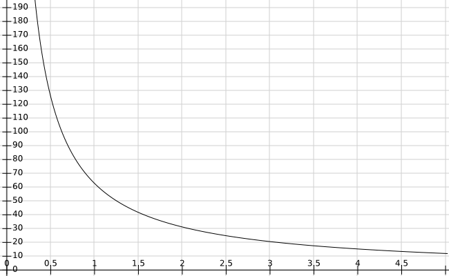
In Sec. V we said that the partition of $SO(2)$ is constructed in such a way that the distance $\Delta\phi$ between two consecutive orientation samples should be chosen such that the maximal displacement does not exceed the chosen $\varepsilon$. Note that $\varepsilon$ should be less than the radius $r$ of the smallest ball in the object’s representation in order to preserve the shape of the object. On the other hand, Fig. 5 shows that the number $s$ grows significantly when we decrease the $\varepsilon$. Finally, the possible choice of $\varepsilon$ depends on the shape of the object: if the shape is easy to approximate with a small number of large balls, then we can choose a large $\varepsilon$ without losing any crucial information about the shape. In contrast, if the object has a lot of thin parts, it has to be approximated with a larger number of smaller balls. In this case we have to choose a smaller $\varepsilon$, which increases the necessary number of slices.

References

- [1] Barraquand, J., Kavraki, L., Latombe, J.-C., Motwani, R., Li, T.-Y., Raghavan, P.: A random sampling scheme for path planning. In: The International Journal of Robotics Research, 16(6), 759–774 (1997).
- [2] Basch, J., Guibas, L. J., Hsu, D., Nguyen, A. T.: Disconnection proofs for motion planning. In: IEEE International Conference on Robotics and Automation (2001), 1765-1772.
- [3] Bullo, F., Lewis, A. D.: Geometric Control of Mechanical Systems. Springer, 2005.
- [4] Edelsbrunner, H., Harer, J.: Computational topology: an introduction. American Mathematical Soc., 2010.
- [5] Guibas, L.J., Stolfi, J.: Primitives for the manipulation of general subdivisions and the computation of Voronoi diagrams. In: ACM Trans. Graphics, 4 (1985), 74-123.
- [6] Kuperberg, W.: Problems on polytopes and convex sets. In: DIMACS Workshop on polytopes (1990), 584-589.
- [7] Latombe, J.-C.: Robot Motion Planning. Norwell, MA, USA: Kluwer Academic Publishers (1991).
- [8] Mahler, J., Pokorny, F. T., McCarthy, Z., van der Stappen, A. F., Goldberg, K.: Energy-bounded caging: Formal definition and 2-D energy lower bound algorithm based on weighted alpha shapes. In: IEEE Robotics and Automation Letters, 1(1), 508-515 (2016).
- [9] Makita, S., Maeda, Y.: 3D multifingered caging: Basic formulation and planning. In: IEEE Intelligent Robots and Systems (2008), 2697–2702.
- [10] Makita, S., Okita, K., Maeda, Y.: 3D two-fingered caging for two types of objects: sufficient conditions and planning. In: International Journal of Mechatronics and Automation, 3(4), 263-277 (2013)
- [11] McCarthy, Z., Bretl, T., Hutchinson, S.: Proving path non-existence using sampling and alpha shapes. In: IEEE International Conference on Robotics and Automation (2012), 2563-2569.
- [12] Pipattanasomporn, P., Sudsang, A.: Two-finger caging of concave polygon. In: IEEE International Conference on Robotics and Automation (2006), 2137–2142.
- [13] Pipattanasomporn, P., Sudsang, A.: Two-finger caging of nonconvex polytopes. In: IEEE Transactions on Robotics, 27(2), 324-333 (2011).
- [14] Pokorny, F. T., Stork, J. A., Kragic, D.: Grasping objects with holes: A topological approach. In: IEEE International Conference on Robotics and Automation (2013), 1100–1107.
- [15] Rimon, E., Blake, A.: Caging planar bodies by one-parameter two-fingered gripping systems. In: The International Journal of Robotics Research, 18(3), 299–318 (1999).
- [16] Rodriguez, A., Mason, M. T., Ferry, S.: From caging to grasping. In: The International Journal of Robotics Research, 31(7), 886-900 (2012).
- [17] Stork, J. A., Pokorny, F. T., Kragic, D.: Integrated Motion and Clasp Planning with Virtual Linking. In: IEEE/RSJ International Conference on Intelligent Robots and Systems (2013), 3007-3014.
- [18] Stork, J. A., Pokorny, F. T., Kragic, D.: A Topology-based Object Representation for Clasping, Latching and Hooking. In: IEEE-RAS International Conference on Humanoid Robots (2013), 138-145.
- [19] Pereira, G. A. S., Campos, M.F.M., Kumar, V.: Decentralized algorithms for multi-robot manipulation via caging. In: The International Journal of Robotics Research 23(7-8), 783 – 795 (2004).
- [20] Varava, A., Kragic, D., Pokorny, F. T.: Caging Grasps of Rigid and Partially Deformable 3-D Objects With Double Fork and Neck Features. In IEEE Transactions on Robotics, 32(6), 1479-1497 (2016).
- [21] Varava, A., Carvalho, J. F., Pokorny, F. T., Kragic, D.: Caging and Path Non-Existence: a Deterministic Sampling-Based Verification Algorithm. International Symposium on Robotics Research, 2017 (accepted, to appear). Preprint: http://www.csc.kth.se/~jfpbdc/path_non_ex.pdf
- [22] Vahedi, M., van der Stappen, A. F.: Caging polygons with two and three fingers. In: The International Journal of Robotics Research, 27(11-12) 1308–1324 (2008).
- [23] Zhang, L., Young, J. K., Manocha, D.: Efficient cell labelling and path non-existence computation using C-obstacle query. In: The International Journal of Robotics Research, 27(11-12), 1246-1257 (2008).