跳到论文正文
W Papers独立论文阅读器 arXiv:1710.09828 论文正文 计算阅读时间 · 0%
引用这篇论文根据当前论文元数据生成,正式投稿前建议核对。


License: arXiv.org perpetual non-exclusive license
arXiv:1710.09828v1 [eess.SY] 26 Oct 2017

Gaussian Process Regression for Generalized Frequency Response Function Estimation

Jeremy Stoddard Affiliation:  University of Newcastle, Callaghan, NSW, Australia    Georgios Birpoutsoukis Affiliation:  Vrije Universiteit Brussel, Brussels, Belgium
August 24, 2026

1 Introduction

Kernel-based modeling of dynamic systems has garnered a significant amount of attention in the system identification literature since its introduction to the field in [7]. While the method was originally applied to linear impulse response estimation in the time domain, the concepts have since been extended to the frequency domain for estimation of frequency response functions (FRFs) [6], as well as to the Volterra series in [1]. In the latter case, smoothness and stable decay was imposed along the hypersurfaces of the multidimensional impulse responses (referred to as ‘Volterra kernels’ in the sequel), allowing lower variance estimates than could be obtained in a simple least squares framework.

The Volterra series can also be expressed in a frequency domain context, however there are several competing representations which all possess some unique advantages [4]. Perhaps the most natural representation is the generalized frequency response function (GFRF), which is defined as the multidimensional Fourier transform of the corresponding Volterra kernel in the time-domain series. The representation leads to a series of frequency domain functions with increasing dimension.

2 Review of GFRFs

2.1 The Volterra Series in the Frequency Domain

We consider the nonlinear systems whose output is described by the discrete time Volterra series given by [9] ,

y0​(k)=∑m=1M[∑τ1=0nm−1…​∑τm=0nm−1hm​(τ1,…,τm)​∏τ=τ1τmu⁡(k−τ)],y^{0}(k)=\sum_{m=1}^{M}\Bigg[\sum_{\tau_{1}=0}^{n_{m}-1}\ldots\sum_{\tau_{m}=0}^{n_{m}-1}h_{m}(\tau_{1},\ldots,\tau_{m})\prod_{\tau=\tau_{1}}^{\tau_{m}}u(k-\tau)\Bigg], (1)

where hm​(τ1,…,τm)h_{m}(\tau_{1},\ldots,\tau_{m}) is the mm’th order Volterra kernel, nmn_{m} is the memory length of hmh_{m}, and τj\tau_{j} is the jj’th lag variable for the kernel. The subscript mm gives the dimension of the kernels, up to a maximum degree, MM.

A steady-state expression for such Volterra series models in the frequency domain was first derived in [5]. For NN-point input and output DFT spectra given by Y⁡(k)Y(k) and U⁡(k)U(k) respectively, the relationship between the two is described by,

Y0​(k)\displaystyle Y^{0}(k) =∑m=1MYm​(k)​∀k,\displaystyle=\sum_{m=1}^{M}Y_{m}(k)\;\;\forall k, (2)
Ym​(k)\displaystyle Y_{m}(k) =∑k1+…+km=kHm​(Ωk1,…,Ωkm)​∏i=1mU⁡(ki),\displaystyle=\sum_{k_{1}+\ldots+k_{m}=k}H_{m}(\Omega_{k_{1}},\ldots,\Omega_{k_{m}})\prod_{i=1}^{m}U(k_{i}), (3)

where Ωk\Omega_{k} is a generic frequency variable corresponding to the kk’th DFT index, and Hm​(Ωk1,…,Ωkm)H_{m}(\Omega_{k_{1}},\ldots,\Omega_{k_{m}}) is labelled the mm’th order GFRF, given by a multidimensional DFT of the mm’th time domain kernel, hmh_{m}, i.e.

Hm​(Ωk1,…,Ωkm)=∑τ1=0nm−1…​∑τm=0nm−1hm​(τ1,…,τm)​e−j​2​π​k1​τ1N​…​e−j​2​π​km​τmN.H_{m}(\Omega_{k_{1}},\ldots,\Omega_{k_{m}})=\sum_{\tau_{1}=0}^{n_{m}-1}\ldots\sum_{\tau_{m}=0}^{n_{m}-1}h_{m}(\tau_{1},\ldots,\tau_{m})e^{\frac{-j2\pi k_{1}\tau_{1}}{N}}\ldots e^{\frac{-j2\pi k_{m}\tau_{m}}{N}}. (4)

A second order example is provided in Figure 1 to compare the two kernel domains. Direct frequency domain estimation of GFRFs is typically very difficult in practice, due to their multidimensional nature and the complexity of the hyperplane sum.

Refer to caption
Figure 1: Time domain kernel (left) and frequency domain GFRF (right) for a second order Wiener-Hammerstein system

3 Regularized Estimation of GFRFs

The concepts introduced in [6] can be extended to estimation of GFRF models, however the covariance functions will differ significantly from the linear case, and the model must now be constructed using a matrix multiplication of the regressor and parameter vector, rather than a simple Hadamard product. This section will describe the Gaussian assumptions on the system, detail the covariance function design and tuning, and derive the maximum a posteriori (MAP) estimates of the GFRFs.

3.1 Complex Normal Distributions

In this paper, we will neglect all DFT indices associated with strictly real spectrum quantities, such that the complex normal distribution is sufficient to describe all Gaussian processes in the system. Relevant notation for such distributions is detailed here.

For a complex Gaussian vector, XX, we define the augmented vector as X~T=[XT​XH]\widetilde{X}^{T}=[X^{T}X^{H}], where (⋅)T(\cdot)^{T} and (⋅)H(\cdot)^{H} denote the transpose and Hermitian transpose of a vector respectively. The distribution of XX is written as,

X∼𝒞​𝒩​(m,Σ)X\sim\mathcal{CN}(m,\Sigma)

where m=E​{X~}m=\textbf{E}\{\widetilde{X}\} and Σ=E​{(X~−m)​(X~−m)H}\Sigma=\textbf{E}\{(\widetilde{X}-m)(\widetilde{X}-m)^{H}\}. The augmented covariance, Σ\Sigma, can be decomposed into covariance and relation function components, KK and CC, as

Σ=[KCCHK¯]\Sigma=\begin{bmatrix}K&C\\ C^{H}&\overline{K}\end{bmatrix}

where K=E​{(X−E​{X})​(X−E​{X})H}K=\textbf{E}\{(X-\textbf{E}\{X\})(X-\textbf{E}\{X\})^{H}\} and C=E​{(X−E​{X})​(X−E​{X})T}C=\textbf{E}\{(X-\textbf{E}\{X\})(X-\textbf{E}\{X\})^{T}\}.

3.2 System Assumptions

For convenient estimation, some assumptions must be made on the system, its Gaussian distributions, and the input excitation.

Assumption 1.

The (discrete) frequency domain description of the system in steady-state can be given as,

Y⁡(k)=∑m=1MYm​(k)+V⁡(k),Ym​(k)=∑k1+…+km=kHm​(Ωk1,…,Ωkm)​∏i=1mU⁡(ki),\begin{split}Y(k)&=\sum_{m=1}^{M}Y_{m}(k)+V(k),\\ Y_{m}(k)&=\sum_{k_{1}+\ldots+k_{m}=k}H_{m}(\Omega_{k_{1}},\ldots,\Omega_{k_{m}})\prod_{i=1}^{m}U(k_{i}),\end{split} (5)

where V⁡(k)V(k) is complex circular output measurement noise with variance σv2\sigma^{2}_{v}.

Assumption 2.

For input and output spectra Y⁡(k)Y(k) and U⁡(k)U(k) computed by an NN-point DFT, the time domain input u⁡(t)u(t) is periodic in NN, i.e.

u⁡(t)=u⁡(t+N)​∀tu(t)=u(t+N)\;\;\;\forall t

This implies that the measured output will be transient-free, since the system is in steady-state with period length equal to the measurement window.

Definition 1.

For an NN-point DFT, the set of DFT indices for which the input spectrum is non-zero is labelled 𝐤𝐮⊂{1,…,N/2​M−1}\mathbf{k_{u}}\subset\{1,\ldots,N/2M-1\}. The corresponding excited indices of the output spectrum are contained in 𝐤𝐲\mathbf{k_{y}}.

Remark 1.

The frequencies excited by the input signal, uu, at which HmH_{m} can be estimated, will be given by the set 𝛀={−Ω𝐤𝐮​Ω𝐤𝐮}\mathbf{\Omega}=\{-\Omega_{\mathbf{k_{u}}}\;\;\Omega_{\mathbf{k_{u}}}\}.

Definition 2.

The mm-dimensional tensor containing Hm​(Ωk1,…,Ωkm)H_{m}(\Omega_{k_{1}},\ldots,\Omega_{k_{m}}) ∀Ωk1,…,Ωkm∈𝛀\forall\Omega_{k_{1}},\ldots,\Omega_{k_{m}}\in\mathbf{\Omega} has a vectorized form which will be denoted by Hm𝒱H_{m}^{\mathcal{V}}. The vectorization scheme remains arbitrary here, but will be discussed in Section 3.3.

Assumption 3.

Hm𝒱H_{m}^{\mathcal{V}} is complex Gaussian distributed with zero mean and augmented covariance Σm\Sigma_{m}, i.e.

Hm𝒱∼𝒞​𝒩​(0,Σm)H_{m}^{\mathcal{V}}\sim\mathcal{CN}(0,\Sigma_{m}) (6)
Assumption 4.

Any two Gaussian GFRFs, Hi𝒱H_{i}^{\mathcal{V}} and Hj𝒱H_{j}^{\mathcal{V}}, are independent for i≠ji\neq j.

3.3 Designing Multidimensional Covariance Functions

For multidimensional Volterra kernels, covariance functions have already been constructed in the time domain [1], by applying a diagonal/correlated (DC) structure [3] along multiple perpendicular ‘regularizing directions.’ The resulting covariance matrices are guaranteed to be valid and produce stable kernel realizations; two properties which we desire in the frequency domain context as well. These functions can be transformed to the frequency domain using a similar approach to that taken in [6], but the transformation will be more complex due to the required vectorization of time and frequency domain quantities in order to produce 2-dimensional covariance matrices. However, if the vectorization scheme is chosen carefully, the transformation matrix will possess a structure useful for software implementation.

In this paper, for a quantity X⁡(i1,…,im)X(i_{1},\ldots,i_{m}) where i1,…,im=0,1,…,N−1i_{1},\ldots,i_{m}=0,1,\ldots,N-1, we define the vectorized quantity, X𝒱X^{\mathcal{V}}, as the vector obtained by first incrementing i1i_{1}, then i2i_{2}, and so on. Now we are interested in finding the matrix, FmF_{m}, which represents the following transformation:

Hm𝒱=Fm​hm𝒱,H_{m}^{\mathcal{V}}=F_{m}h_{m}^{\mathcal{V}},

where HmH_{m} is the multidimensional Fourier transform of Volterra kernel hmh_{m}. Under the considered vectorization scheme, FmF_{m} can be constructed recursively from the N×NN\times N DFT matrix, which we denote F1F_{1}. The result is a matrix which retains the neat structure and symmetries of the 1-dimensional transform, as noted in [2]. The recursive definition can be written as,

Fm=[Fm−1​(1,1)⋅F1…Fm−1​(1,Nm−1)⋅F1⋱Fm−1​(Nm−1,1)⋅F1…Fm−1​(Nm−1,Nm−1)⋅F1],m=2,3,…F_{m}=\begin{bmatrix}F_{m-1}(1,1)\cdot F_{1}&\ldots&F_{m-1}(1,N^{m-1})\cdot F_{1}\\ \vdots&\ddots&\vdots\\ F_{m-1}(N^{m-1},1)\cdot F_{1}&\ldots&F_{m-1}(N^{m-1},N^{m-1})\cdot F_{1}\end{bmatrix},\;\;\;\;m=2,3,\ldots

where Fm​(i,j)F_{m}(i,j) indicates the i,ji,j’th element of matrix FmF_{m}.

The vectorized transformation can now be used to convert time domain covariance functions to the frequency domain as follows,

Km\displaystyle K_{m} =E​{Hm𝒱​Hm𝒱H}=Fm​E​{hm𝒱​hm𝒱T}​FmH=Fm​Pm​FmH\displaystyle=\textbf{E}\{H_{m}^{\mathcal{V}}{H_{m}^{\mathcal{V}}}^{H}\}=F_{m}\textbf{E}\{h_{m}^{\mathcal{V}}{h_{m}^{\mathcal{V}}}^{T}\}F_{m}^{H}=F_{m}P_{m}F_{m}^{H} (7)
Cm\displaystyle C_{m} =E​{Hm𝒱​Hm𝒱T}=Fm​E​{hm𝒱​hm𝒱T}​FmT=Fm​Pm​Fm\displaystyle=\textbf{E}\{H_{m}^{\mathcal{V}}{H_{m}^{\mathcal{V}}}^{T}\}=F_{m}\textbf{E}\{h_{m}^{\mathcal{V}}{h_{m}^{\mathcal{V}}}^{T}\}F_{m}^{T}=F_{m}P_{m}F_{m} (8)

where PmP_{m} denotes the DC-based covariance structure of vectorized kernel hm𝒱h_{m}^{\mathcal{V}} as designed in [1].

Remark 2.

In practice, symmetry must be enforced in both the time and frequency domain kernels to guarantee a unique Volterra series representation. This requires some modification of the transformation matrices, FmF_{m}, in order to consider only the unique components of each kernel.

3.3.1 The Output Spectrum

The output spectrum of Y⁡(𝐤𝐲)Y(\mathbf{k_{y}}) can now be derived in a similar fashion to the linear case. However, we must first restructure the model equation, (5), into a least squares framework, i.e.

Y⁡(𝐤𝐲)=[ϕ1​…​ϕM]​[H1𝒱T​…​HM𝒱T]T+V⁡(𝐤𝐲)=ϕ​H+V,Y(\mathbf{k_{y}})=[\phi_{1}\ldots\phi_{M}][{H_{1}^{\mathcal{V}}}^{T}\ldots{H_{M}^{\mathcal{V}}}^{T}]^{T}+V(\mathbf{k_{y}})=\phi H+V,

where ϕm\phi_{m} is an appropriate regressor containing the input spectrum products corresponding to Hm∗H_{m}^{*}. Note that symmetry should also be enforced in the GFRFs here, which should be reflected in the design of the regressors. Extending this equation to the augmented output case gives,

Y~​(𝐤𝐲)=[ϕ1~​…​ϕM~]​[H1𝒱~T​…​HM𝒱~T]T+V~​(𝐤𝐲)=ϕ~​H~+V~\widetilde{Y}(\mathbf{k_{y}})=[\widetilde{\phi_{1}}\ldots\widetilde{\phi_{M}}][\widetilde{H_{1}^{\mathcal{V}}}^{T}\ldots\widetilde{H_{M}^{\mathcal{V}}}^{T}]^{T}+\widetilde{V}(\mathbf{k_{y}})=\widetilde{\phi}\widetilde{H}+\widetilde{V} (9)

where the augmented regressors are defined by

ϕm~=[ϕm00ϕm¯].\widetilde{\phi_{m}}=\begin{bmatrix}\phi_{m}&0\\ 0&\overline{\phi_{m}}\end{bmatrix}.

From (9), we can now derive the distribution of the output spectrum.

Theorem 1.

For a system given by (5) with Gaussian Hm𝒱H_{m}^{\mathcal{V}} as described in (6), the output spectrum Y⁡(𝐤𝐲)Y(\mathbf{k_{y}}) is complex normally distributed as,

Y⁡(𝐤𝐲)∼𝒞​𝒩​(0,ΣY),where ​ΣY=ϕ~​Σt​o​t​ϕ~H+σv2​Iand ​Σt​o​t=[Σ10⋱0ΣM]\begin{split}Y(\mathbf{k_{y}})&\sim\mathcal{CN}(0,\Sigma_{Y}),\\ \text{where }\Sigma_{Y}&=\widetilde{\phi}\Sigma_{tot}\widetilde{\phi}^{H}+\sigma^{2}_{v}I\\ \text{and }\Sigma_{tot}&=\begin{bmatrix}\Sigma_{1}&&0\\ &\ddots&\\ 0&&\Sigma_{M}\end{bmatrix}\end{split} (10)
Proof.

Follows from the model equation in (9), Assumptions 3 and 4, and the properties of complex normal distributions. ∎

3.4 MAP Estimates of the GFRFs

MAP estimates can be obtained from the joint distribution of YY and HH, by computing the mean of the conditional distribution H|YH|Y. The result is provided in the following theorem.

Theorem 2.

The MAP estimate of H~\widetilde{H} in (9) is given by

H~^M​A​P=Σt​o​t​ϕ~H​ΣY−1​Y~\hat{{\widetilde{H}}}_{MAP}=\Sigma_{tot}\widetilde{\phi}^{H}\Sigma_{Y}^{-1}\widetilde{Y} (11)
Proof.

Follows from the properties of joint complex distributions. ∎

3.5 Hyperparameter Tuning using Marginal Likelihood

Optimization of the hyperparameters describing each Gaussian process can be performed using the exact same methodology employed in [6], by maximizing the log marginal likelihood, i.e.

η^=arg ​min 𝜂​Y~​(𝐤𝐲)H​ΣY−1​(η)​Y~​(𝐤𝐲)+log det ​ΣY​(η).\hat{\eta}=\text{arg }\underset{\eta}{\text{min }}\widetilde{Y}(\mathbf{k_{y}})^{H}\Sigma_{Y}^{-1}(\eta)\widetilde{Y}(\mathbf{k_{y}})+\text{log det }\Sigma_{Y}(\eta).

The only notable difference is in the construction of ΣY\Sigma_{Y}, which is now formed using the complex regressor, ϕ~\widetilde{\phi}, and a block-diagonal combination of each GFRFs covariance matrix.

It is important to note that the covariance matrices are first computed in the time domain as PmP_{m}, then transformed into the augmented frequency domain covariance, Σm\Sigma_{m}, using transformation matrices FmF_{m} as outlined in Section 3.3.

4 Numerical Examples

To demonstrate the estimation performance of Gaussian process regression for GFRFs, several systems with different nonlinear dynamics were simulated. The systems were all block-oriented in nature; Wiener, Hammerstein, and Wiener-Hammerstein, and the static nonlinear block had the form f⁡(x)=x2f(x)=x^{2} in each case. This results in systems which contain only second order Volterra series terms.

Refer to caption
Figure 2: True (transparent) and estimated GFRFs for a Hammerstein system

The input was constructed as a random-phase multisine of length N=55N=55 with 13 excited frequencies, allowing the estimation of 182182 unique GFRF parameters in each case. No measurement noise was added to the output spectrum, but Gaussian process regression is still required due to the rank deficiency of the estimation problem. For each nonlinear block structure, the resulting estimates have their magnitude plotted in Figures 2, 3 and 4 for a single input realization. The estimates are plotted on top of the true GFRF (transparent) for comparison, revealing a close match in each case. It is clear that tuning and transforming the time-domain covariance structures from [1] leads to satisfactory GFRF estimation, even when the problem is severely rank deficient.

Refer to caption
Figure 3: True (transparent) and estimated GFRFs for a Wiener system
Refer to caption
Figure 4: True (transparent) and estimated GFRFs for a Wiener-Hammerstein system

5 Transients in a Second Order Volterra System

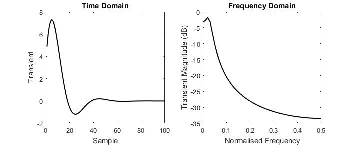
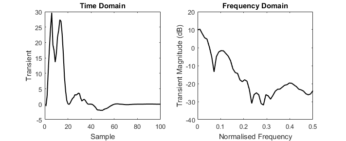
While all previous results in this paper relied on the assumption of transient-free measurements from a periodic input excitation, one major benefit of Gaussian process regression for linear FRFs was the ability to estimate and remove transient functions for the non-periodic input case. However, this is only made possible by the approximation that the covariance of the transient function is a scaled version of the system covariance. While the approximation is well justified in the linear case, the same cannot be said in general for 2nd and higher order Volterra systems. The increased complexity of nonlinear transients can be observed in the examples of Figures 5 and 6, which show transients resulting from a linear system and its second order Wiener counterpart.
Refer to caption
Figure 5: Transient resulting from zero initial conditions in a linear filter
Refer to caption
Figure 6: Transient resulting from zero initial conditions in a second order Wiener system

In order to understand why this is the case, we first summarise the transient derivation for a linear system, and then derive an analytic expression for the transient response of a system whose output is described by a second order Volterra kernel.

5.1 Transient Expression for a Linear System

The following is a summary of the derivation which can be found in [6]. Consider a linear system described by its infinite impulse response, hh, as,

y⁡(t)=∑n=0∞h⁡(n)​u​(t−n),y(t)=\sum_{n=0}^{\infty}h(n)u(t-n),

where uu and yy are the input and output of the system respectively. It can be shown that the NN-point DFT of y⁡(t),t=0,1,…,N−1y(t),t=0,1,\ldots,N-1, which we will denote Y⁡(k)Y(k), is related to the corresponding input DFT, U⁡(k)U(k), in the following way [8]:

Y⁡(k)\displaystyle Y(k) =∑n=0∞h⁡(n)​e−j​2​π​k​nN​∑t=0N−1u⁡(t)​e−j​2​π​k​tN+T⁡(k)\displaystyle=\sum_{n=0}^{\infty}h(n)e^{\frac{-j2\pi kn}{N}}\sum_{t=0}^{N-1}u(t)e^{\frac{-j2\pi kt}{N}}+T(k)
=H⁡(k)​U​(k)+T⁡(k),\displaystyle=H(k)U(k)+T(k),

where H⁡(k)​U​(k)H(k)U(k) describes the steady state response to uu, and T⁡(k)T(k) is a transient function given by ([6]),

T⁡(k)\displaystyle T(k) =∑t=0∞∑n=t+1∞h⁡(n)​f​(t−n)⏟h∗​(t)​e−j​2​π​k​tN\displaystyle=\sum_{t=0}^{\infty}\underbrace{\sum_{n=t+1}^{\infty}h(n)f(t-n)}_{h^{*}(t)}e^{\frac{-j2\pi kt}{N}} (12)
where ​f​(t)\displaystyle\textrm{where }f(t) =u⁡(t)−u⁡(t+N).\displaystyle=u(t)-u(t+N).

The term h∗​(t)h^{*}(t) is seen to be a free response of the system with impulse response hnh_{n}.

5.2 Derivation of the Second Order Transient Expression

Consider the noiseless output of a nonlinear system described by a second order Volterra kernel, i.e.

y⁡(t)=∑τ1=0∞∑τ2=0∞h2​(τ1,τ2)​u​(t−τ1)​u​(t−τ2)y(t)=\sum\limits_{\tau_{1}=0}^{\infty}\sum\limits_{\tau_{2}=0}^{\infty}h_{2}(\tau_{1},\tau_{2})u(t-\tau_{1})u(t-\tau_{2}) (13)

Assume that NN samples of the input uu and output yy are available. Applying a DFT on the measured output signal y⁡(t),t=0,1,…,N−1y(t),t=0,1,\ldots,N-1, the spectral component of yy at DFT frequency kk is given by,

Y⁡(k)=∑t=0N−1y⁡(t)​e−j​ωk​t=∑t=0N−1(∑τ1=0∞∑τ2=0∞h2​(τ1,τ2)​u​(t−τ1)​u​(t−τ2))​e−j​ωk​t,Y(k)=\sum\limits_{t=0}^{N-1}y(t)e^{-j\omega_{k}t}=\sum\limits_{t=0}^{N-1}(\sum\limits_{\tau_{1}=0}^{\infty}\sum\limits_{\tau_{2}=0}^{\infty}h_{2}(\tau_{1},\tau_{2})u(t-\tau_{1})u(t-\tau_{2}))e^{-j\omega_{k}t}, (14)

where ωk=2​π​kN\omega_{k}=\frac{2\pi k}{N}. The term e−j​ωk​te^{-j\omega_{k}t} can be split as follows:

e−j​ωk​t\displaystyle e^{-j\omega_{k}t} =e−j​ωk1​τ1​e−j​ωk−k1​τ2​e−j​ωk1​(t−τ1)​e−j​ωk−k1​(t−τ2)\displaystyle=e^{-j\omega_{k_{1}}\tau_{1}}e^{-j\omega_{k-k_{1}}\tau_{2}}e^{-j\omega_{k_{1}}(t-\tau_{1})}e^{-j\omega_{k-k_{1}}(t-\tau_{2})} (15)
withωk1+ωk−k1=ωk\displaystyle\textrm{with}\ \ \omega_{k_{1}}+\omega_{k-k_{1}}=\omega_{k}

Moreover, it holds that:

∑t=0N−1u⁡(t−τ1)​e−j​ωk1​t=e−j​ωk1​τ1​(∑t=0N−1u⁡(t−τ1)​e−j​ωk1​(t−τ1))\displaystyle\sum\limits_{t=0}^{N-1}u(t-\tau_{1})e^{-j\omega_{k_{1}}t}=e^{-j\omega_{k_{1}}\tau_{1}}\bigg(\sum\limits_{t=0}^{N-1}u(t-\tau_{1})e^{-j\omega_{k_{1}}(t-\tau_{1})}\bigg)
=e−j​ωk1​τ1​(∑t=0N−1u⁡(t)​e−j​ωk1​t⏟U⁡(k1)+∑t=−τ1−1(u⁡(t)−u⁡(t+N))​e−j​ωk1​t)⇔\displaystyle=e^{-j\omega_{k_{1}}\tau_{1}}\bigg(\underbrace{\sum\limits_{t=0}^{N-1}u(t)e^{-j\omega_{k_{1}}t}}_{U(k_{1})}+\sum\limits_{t=-\tau_{1}}^{-1}(u(t)-u(t+N))e^{-j\omega_{k_{1}}t}\bigg)\Leftrightarrow
∑t=0N−1u⁡(t−τ1)​e−j​ωk1​(t−τ1)⏟Ut−τ1​(k1)=U⁡(k1)+∑t=−τ1−1(u⁡(t)−u⁡(t+N))​e−j​ωk1​t⇔\displaystyle\underbrace{\sum\limits_{t=0}^{N-1}u(t-\tau_{1})e^{-j\omega_{k_{1}}(t-\tau_{1})}}_{U_{t-\tau_{1}}(k_{1})}=U(k_{1})+\sum\limits_{t=-\tau_{1}}^{-1}(u(t)-u(t+N))e^{-j\omega_{k_{1}}t}\Leftrightarrow
Ut−τ1​(k1)=U⁡(k1)+∑t=−τ1−1(u⁡(t)−u⁡(t+N))​e−j​ωk1​tor\displaystyle U_{t-\tau_{1}}(k_{1})=U(k_{1})+\sum\limits_{t=-\tau_{1}}^{-1}(u(t)-u(t+N))e^{-j\omega_{k_{1}}t}\ \ \ \ \ \ \ \ \textrm{or}
u⁡(t−τ1)\displaystyle u(t-\tau_{1}) =∑k1=0N−1Ut−τ1​(k1)​ej​ωk1​(t−τ1)⇔\displaystyle=\sum\limits_{k_{1}=0}^{N-1}U_{t-\tau_{1}}(k_{1})e^{j\omega_{k_{1}}(t-\tau_{1})}\Leftrightarrow (16)
u⁡(t−τ1)\displaystyle u(t-\tau_{1}) =∑k1=0N−1(U⁡(k1)+∑t=−τ1−1(u⁡(t)−u⁡(t+N))​e−j​ωk1​t)​ej​ωk1​(t−τ1)\displaystyle=\sum\limits_{k_{1}=0}^{N-1}\bigg(U(k_{1})+\sum\limits_{t=-\tau_{1}}^{-1}(u(t)-u(t+N))e^{-j\omega_{k_{1}}t}\bigg)e^{j\omega_{k_{1}}(t-\tau_{1})}

Similarly it can be derived that:

∑t=0N−1u⁡(t−τ2)​e−j​ωk−k1​(t−τ2)=U⁡(k−k1)+∑t=−τ2−1(u⁡(t)−u⁡(t+N))​e−j​ωk−k1​t\sum\limits_{t=0}^{N-1}u(t-\tau_{2})e^{-j\omega_{k-k_{1}}(t-\tau_{2})}=U(k-k_{1})+\sum\limits_{t=-\tau_{2}}^{-1}(u(t)-u(t+N))e^{-j\omega_{k-k_{1}}t} (17)

After substituting (15), (16) and (17) into (14) we obtain:

Y⁡(k)\displaystyle Y(k) =∑k1=0N−1∑τ1=0∞∑τ2=0∞h2​(τ1,τ2)​e−j​ωk1​τ1​e−j​ωk−k1​τ2\displaystyle=\sum\limits_{k_{1}=0}^{N-1}\sum\limits_{\tau_{1}=0}^{\infty}\sum\limits_{\tau_{2}=0}^{\infty}h_{2}(\tau_{1},\tau_{2})e^{-j\omega_{k_{1}}\tau_{1}}e^{-j\omega_{k-k_{1}}\tau_{2}}
…(U(k1)+∑t′=−τ1−1(u(t′)−u(t′+N)⏟f(t′))e−jωk1t′)\displaystyle\ldots\bigg(U(k_{1})+\sum\limits_{t^{{}^{\prime}}=-\tau_{1}}^{-1}(\underbrace{u(t^{{}^{\prime}})-u(t^{{}^{\prime}}+N)}_{f(t^{{}^{\prime}})})e^{-j\omega_{k_{1}}t^{{}^{\prime}}}\bigg)
…(U(k−k1)+∑t′′=−τ2−1(u(t′′)−u(t′′+N)⏟f(t′′))e−jωk−k1t′′)⇔\displaystyle\ldots\bigg(U(k-k_{1})+\sum\limits_{t^{{}^{\prime\prime}}=-\tau_{2}}^{-1}(\underbrace{u(t^{{}^{\prime\prime}})-u(t^{{}^{\prime\prime}}+N)}_{f(t^{{}^{\prime\prime}})})e^{-j\omega_{k-k_{1}}t^{{}^{\prime\prime}}}\bigg)\Leftrightarrow
Y⁡(k)\displaystyle Y(k) =∑k1=0N−1(∑τ1=0∞∑τ2=0∞h2​(τ1,τ2)​e−j​ωk1​τ1​e−j​ωk−k1​τ2⏟H2​(k1,k−k1))​U​(k1)​U​(k−k1)⏟Steady state response or​S​S\displaystyle=\underbrace{\sum\limits_{k_{1}=0}^{N-1}\bigg(\underbrace{\sum\limits_{\tau_{1}=0}^{\infty}\sum\limits_{\tau_{2}=0}^{\infty}h_{2}(\tau_{1},\tau_{2})e^{-j\omega_{k_{1}}\tau_{1}}e^{-j\omega_{k-k_{1}}\tau_{2}}}_{H_{2}(k_{1},k-k_{1})}\bigg)U(k_{1})U(k-k_{1})}_{\textrm{Steady state response or}\ SS} (18)
+∑k1=0N−1∑τ1=0∞∑τ2=0∞h2(τ1,τ2)e−j​ωk1​τ1e−j​ωk−k1​τ2U(k1)∑t′′=−τ2−1f(t′′)e−jωk−k1t′′⏟Transient term 1 or​T1\displaystyle+\underbrace{\sum\limits_{k_{1}=0}^{N-1}\sum\limits_{\tau_{1}=0}^{\infty}\sum\limits_{\tau_{2}=0}^{\infty}h_{2}(\tau_{1},\tau_{2})e^{-j\omega_{k_{1}}\tau_{1}}e^{-j\omega_{k-k_{1}}\tau_{2}}U(k_{1})\sum\limits_{t^{{}^{\prime\prime}}=-\tau_{2}}^{-1}f(t^{{}^{\prime\prime}})e^{-j\omega_{k-k_{1}}t^{{}^{\prime\prime}}}}_{\textrm{Transient term 1 or}\ T_{1}}
+∑k1=0N−1∑τ1=0∞∑τ2=0∞h2(τ1,τ2)e−j​ωk1​τ1e−j​ωk−k1​τ2U(k−k1)∑t′=−τ1−1f(t′)e−jωk1t′⏟Transient term 2 or​T2\displaystyle+\underbrace{\sum\limits_{k_{1}=0}^{N-1}\sum\limits_{\tau_{1}=0}^{\infty}\sum\limits_{\tau_{2}=0}^{\infty}h_{2}(\tau_{1},\tau_{2})e^{-j\omega_{k_{1}}\tau_{1}}e^{-j\omega_{k-k_{1}}\tau_{2}}U(k-k_{1})\sum\limits_{t^{{}^{\prime}}=-\tau_{1}}^{-1}f(t^{{}^{\prime}})e^{-j\omega_{k_{1}}t^{{}^{\prime}}}}_{\textrm{Transient term 2 or}\ T_{2}}
+∑k1=0N−1∑τ1=0∞∑τ2=0∞h2(τ1,τ2)e−j​ωk1​τ1e−j​ωk−k1​τ2×\displaystyle+\sum\limits_{k_{1}=0}^{N-1}\sum\limits_{\tau_{1}=0}^{\infty}\sum\limits_{\tau_{2}=0}^{\infty}h_{2}(\tau_{1},\tau_{2})e^{-j\omega_{k_{1}}\tau_{1}}e^{-j\omega_{k-k_{1}}\tau_{2}}\times
×∑t′=−τ1−1f(t′)e−jωk1t′∑t′′=−τ2−1f(t′′)e−jωk−k1t′′⏟Transient term 3 or​T3\displaystyle\times\underbrace{\sum\limits_{t^{{}^{\prime}}=-\tau_{1}}^{-1}f(t^{{}^{\prime}})e^{-j\omega_{k_{1}}t^{{}^{\prime}}}\sum\limits_{t^{{}^{\prime\prime}}=-\tau_{2}}^{-1}f(t^{{}^{\prime\prime}})e^{-j\omega_{k-k_{1}}t^{{}^{\prime\prime}}}}_{\textrm{Transient term 3 or}\ T_{3}}

which can be written compactly as:

Y⁡(k)\displaystyle Y(k) =S​S​(k)+T1​(k)+T2​(k)+T3​(k)⏟T⁡(k)\displaystyle=SS(k)+\underbrace{T_{1}(k)+T_{2}(k)+T_{3}(k)}_{T(k)} (19)
S​S​(k)\displaystyle SS(k) =∑k1=0N−1H2​(k1,k−k1)​U​(k1)​U​(k−k1)\displaystyle=\sum\limits_{k_{1}=0}^{N-1}H_{2}(k_{1},k-k_{1})U(k_{1})U(k-k_{1})
T1​(k)\displaystyle T_{1}(k) =∑k1=0N−1∑τ1=0∞∑τ2=0∞h2(τ1,τ2)e−j​ωk1​τ1e−j​ωk−k1​τ2∑t′=0N−1u(t′)e−jωk1t′×\displaystyle=\sum\limits_{k_{1}=0}^{N-1}\sum\limits_{\tau_{1}=0}^{\infty}\sum\limits_{\tau_{2}=0}^{\infty}h_{2}(\tau_{1},\tau_{2})e^{-j\omega_{k_{1}}\tau_{1}}e^{-j\omega_{k-k_{1}}\tau_{2}}\sum\limits_{t^{{}^{\prime}}=0}^{N-1}u(t^{{}^{\prime}})e^{-j\omega_{k_{1}}t^{{}^{\prime}}}\times
×∑t′′=−τ2−1f(t′′)e−jωk−k1t′′\displaystyle\times\sum\limits_{t^{{}^{\prime\prime}}=-\tau_{2}}^{-1}f(t^{{}^{\prime\prime}})e^{-j\omega_{k-k_{1}}t^{{}^{\prime\prime}}}
=∑k1=0N−1∑t′=0∞∑t′′=0∞[∑τ1=t′+1−Nt′∑τ2=t′′+1∞h2(τ1,τ2)u(t′−τ1)f(t′′−τ2)]⏟h1∗​(t′,t′′)×\displaystyle=\sum\limits_{k_{1}=0}^{N-1}\sum\limits_{t^{{}^{\prime}}=0}^{\infty}\sum\limits_{t^{{}^{\prime\prime}}=0}^{\infty}\underbrace{\Bigg[\sum\limits_{\tau_{1}=t^{{}^{\prime}}+1-N}^{t^{{}^{\prime}}}\sum\limits_{\tau_{2}=t^{{}^{\prime\prime}}+1}^{\infty}h_{2}(\tau_{1},\tau_{2})u(t^{{}^{\prime}}-\tau_{1})f(t^{{}^{\prime\prime}}-\tau_{2})\Bigg]}_{h_{1}^{*}(t^{\prime},t^{\prime\prime})}\times
×e−jωk1t′e−jωk−k1t′′\displaystyle\times e^{-j\omega_{k_{1}}t^{{}^{\prime}}}e^{-j\omega_{k-k_{1}}t^{{}^{\prime\prime}}}
T2​(k)\displaystyle T_{2}(k) =∑k1=0N−1∑τ1=0∞∑τ2=0∞h2(τ1,τ2)e−j​ωk1​τ1e−j​ωk−k1​τ2∑t′′=0N−1u(t′′)e−jωk−k1t′′×\displaystyle=\sum\limits_{k_{1}=0}^{N-1}\sum\limits_{\tau_{1}=0}^{\infty}\sum\limits_{\tau_{2}=0}^{\infty}h_{2}(\tau_{1},\tau_{2})e^{-j\omega_{k_{1}}\tau_{1}}e^{-j\omega_{k-k_{1}}\tau_{2}}\sum\limits_{t^{{}^{\prime\prime}}=0}^{N-1}u(t^{{}^{\prime\prime}})e^{-j\omega_{k-k_{1}}t^{{}^{\prime\prime}}}\times
×∑t′=−τ1−1f(t′)e−jωk1t′\displaystyle\times\sum\limits_{t^{{}^{\prime}}=-\tau_{1}}^{-1}f(t^{{}^{\prime}})e^{-j\omega_{k_{1}}t^{{}^{\prime}}}
=∑k1=0N−1∑t′=0∞∑t′′=0∞[∑τ1=t′+1∞∑τ2=t′′+1−Nt′′h2(τ1,τ2)f(t′−τ1)u(t′′−τ2)]⏟h2∗​(t′,t′′)×\displaystyle=\sum\limits_{k_{1}=0}^{N-1}\sum\limits_{t^{{}^{\prime}}=0}^{\infty}\sum\limits_{t^{{}^{\prime\prime}}=0}^{\infty}\underbrace{\Bigg[\sum\limits_{\tau_{1}=t^{{}^{\prime}}+1}^{\infty}\sum\limits_{\tau_{2}=t^{{}^{\prime\prime}}+1-N}^{t^{{}^{\prime\prime}}}h_{2}(\tau_{1},\tau_{2})f(t^{{}^{\prime}}-\tau_{1})u(t^{{}^{\prime\prime}}-\tau_{2})\Bigg]}_{h_{2}^{*}(t^{\prime},t^{\prime\prime})}\times
×e−jωk1t′e−jωk−k1t′′\displaystyle\times e^{-j\omega_{k_{1}}t^{{}^{\prime}}}e^{-j\omega_{k-k_{1}}t^{{}^{\prime\prime}}}
T3​(k)\displaystyle T_{3}(k) =∑k1=0N−1∑t′=0∞∑t′′=0∞[∑τ1=t′+1∞∑τ2=t′′+1∞h2(τ1,τ2)f(t′−τ1)f(t′′−τ2)]⏟h3∗​(t′,t′′)×\displaystyle=\sum\limits_{k_{1}=0}^{N-1}\sum\limits_{t^{{}^{\prime}}=0}^{\infty}\sum\limits_{t^{{}^{\prime\prime}}=0}^{\infty}\underbrace{\Bigg[\sum\limits_{\tau_{1}=t^{{}^{\prime}}+1}^{\infty}\sum\limits_{\tau_{2}=t^{{}^{\prime\prime}}+1}^{\infty}h_{2}(\tau_{1},\tau_{2})f(t^{{}^{\prime}}-\tau_{1})f(t^{{}^{\prime\prime}}-\tau_{2})\Bigg]}_{h_{3}^{*}(t^{\prime},t^{\prime\prime})}\times
×e−jωk1t′e−jωk−k1t′′\displaystyle\times e^{-j\omega_{k_{1}}t^{{}^{\prime}}}e^{-j\omega_{k-k_{1}}t^{{}^{\prime\prime}}}

5.3 Equality of the transient terms T1T_{1} and T2T_{2}

Consider the term T1T_{1} as written in (18), and apply the change of variables k−k1=k1′⇔k1=k−k1′k-k_{1}=k_{1}^{{}^{\prime}}\Leftrightarrow k_{1}=k-k_{1}^{{}^{\prime}}. Moreover, interchange τ1\tau_{1} with τ2\tau_{2} due to the symmetry of h2​(τ1,τ2)=h2​(τ2,τ1),∀τ1,τ2h_{2}(\tau_{1},\tau_{2})=h_{2}(\tau_{2},\tau_{1}),\forall\tau_{1},\tau_{2}:

T1​(k)\displaystyle T_{1}(k) =∑k1=0N−1∑τ1=0∞∑τ2=0∞h2(τ1,τ2)e−j​ωk1​τ2e−j​ωk−k1​τ1U(k1)∑t′′=−τ1−1f(t′′)e−jωk−k1t′′\displaystyle=\sum\limits_{k_{1}=0}^{N-1}\sum\limits_{\tau_{1}=0}^{\infty}\sum\limits_{\tau_{2}=0}^{\infty}h_{2}(\tau_{1},\tau_{2})e^{-j\omega_{k_{1}}\tau_{2}}e^{-j\omega_{k-k_{1}}\tau_{1}}U(k_{1})\sum\limits_{t^{{}^{\prime\prime}}=-\tau_{1}}^{-1}f(t^{{}^{\prime\prime}})e^{-j\omega_{k-k_{1}}t^{{}^{\prime\prime}}} (20)
=∑k1′=k+1−Nk∑τ1=0∞∑τ2=0∞h2(τ1,τ2)e−jωk−k1′τ2e−jωk1′τ1∑t′′=−τ1−1f(t′′)e−jωk1′t′′U(k−k1′)\displaystyle=\sum\limits_{k_{1}^{{}^{\prime}}=k+1-N}^{k}\sum\limits_{\tau_{1}=0}^{\infty}\sum\limits_{\tau_{2}=0}^{\infty}h_{2}(\tau_{1},\tau_{2})e^{-j\omega_{k-k_{1}^{{}^{\prime}}}\tau_{2}}e^{-j\omega_{k_{1}^{{}^{\prime}}}\tau_{1}}\sum\limits_{t^{{}^{\prime\prime}}=-\tau_{1}}^{-1}f(t^{{}^{\prime\prime}})e^{-j\omega_{k_{1}^{{}^{\prime}}}t^{{}^{\prime\prime}}}U(k-k_{1}^{{}^{\prime}})

Comparing the latter expression with the equivalent T2T_{2} formulation,

T2​(k)\displaystyle T_{2}(k) =∑k1=0N−1∑τ1=0∞∑τ2=0∞h2(τ1,τ2)e−j​ωk−k1​τ2e−j​ωk1​τ1∑t′=−τ1−1f(t′)e−jωk1t′U(k−k1),\displaystyle=\sum\limits_{k_{1}=0}^{N-1}\sum\limits_{\tau_{1}=0}^{\infty}\sum\limits_{\tau_{2}=0}^{\infty}h_{2}(\tau_{1},\tau_{2})e^{-j\omega_{k-k_{1}}\tau_{2}}e^{-j\omega_{k_{1}}\tau_{1}}\sum\limits_{t^{{}^{\prime}}=-\tau_{1}}^{-1}f(t^{{}^{\prime}})e^{-j\omega_{k_{1}}t^{{}^{\prime}}}U(k-k_{1}), (21)

we see that they differ only in the summation bounds of k1′k_{1}^{{}^{\prime}}. However, consider the following two facts:

  • •

    The DFT of the input signal u⁡(t)u(t) is periodic in the number of samples NN, namely U⁡(k)=U⁡(k+N)U(k)=U(k+N). This implies that ∑k1=0N−1U⁡(k−k1)=∑k1=MM+N−1U⁡(k−k1),∀M\sum\limits_{k_{1}=0}^{N-1}U(k-k_{1})=\sum\limits_{k_{1}=M}^{M+N-1}U(k-k_{1}),\ \forall M. By setting M=k+1−NM=k+1-N we obtain ∑k1=0N−1U⁡(k−k1)=∑k1=k+1−NkU⁡(k−k1)\sum\limits_{k_{1}=0}^{N-1}U(k-k_{1})=\sum\limits_{k_{1}=k+1-N}^{k}U(k-k_{1}).

  • •

    The compex exponential function ej​2​π​kN​te^{j\frac{2\pi k}{N}t} is also periodic in NN since ej​2​π​(k+z∗N)N​t=ej​2​π​kN​t,∀z∈ℤe^{j\frac{2\pi(k+z*N)}{N}t}=e^{j\frac{2\pi k}{N}t},\forall z\in\mathbb{Z}

Under these conditions, it is clear that we can shift the summation bounds of k1′k_{1}^{{}^{\prime}} without consequence, such that

T1​(k)\displaystyle T_{1}(k) =∑k1′=0N−1∑τ1=0∞∑τ2=0∞h2(τ1,τ2)e−jωk−k1′τ2e−jωk1′τ1∑t′′=−τ1−1f(t′′)e−jωk1′t′′U(k−k1′)\displaystyle=\sum\limits_{k_{1}^{{}^{\prime}}=0}^{N-1}\sum\limits_{\tau_{1}=0}^{\infty}\sum\limits_{\tau_{2}=0}^{\infty}h_{2}(\tau_{1},\tau_{2})e^{-j\omega_{k-k_{1}^{{}^{\prime}}}\tau_{2}}e^{-j\omega_{k_{1}^{{}^{\prime}}}\tau_{1}}\sum\limits_{t^{{}^{\prime\prime}}=-\tau_{1}}^{-1}f(t^{{}^{\prime\prime}})e^{-j\omega_{k_{1}^{{}^{\prime}}}t^{{}^{\prime\prime}}}U(k-k_{1}^{{}^{\prime}}) (22)
=T2​(k)\displaystyle=T_{2}(k)

5.4 Qualitative Discussion of Transient Terms

The analysis of the previous sections revealed that in the second order case, the formulation of the transient is significantly more complex than the linear case. In the frequency domain, the total transient can be viewed as the sum of three components, each of which comes from a two-dimensional time domain response that has been transformed and collapsed.

The first two responses, h1∗h^{*}_{1} and h2∗h^{*}_{2}, are asymmetric quantities which provide equal contributions to the transient, and depend directly on the input inside the measured window. The third response, h3∗h_{3}^{*}, represents a natural extension of the linear transient expression in (12), and consequently maintains the desirable property of having similar structure to the underlying system response, h2​(τ1,τ2)h_{2}(\tau_{1},\tau_{2}). Consequently, the corresponding output transient, T3​(k)T_{3}(k), will also share the smoothness properties of linear transients. Example responses are visible in Figure 7 for a second order Wiener system, showing the contrast in complexity between h3∗h_{3}^{*} and the assymetric h1∗h_{1}^{*}. The resulting frequency domain functions, T1​(k)T_{1}(k), T3​(k)T_{3}(k) and T⁡(k)T(k), are plotted in Figure 8 for two Gaussian input realizations.

Refer to caption
Figure 7: The 2-dimensional time domain transient components for a Wiener system

In general, the existence of the h1∗h^{*}_{1} and h2∗h^{*}_{2} terms will complicate the form of the transient in time and frequency domains, which in turn necessitates more sophisticated algorithms for detecting and removing the transient function. As the nonlinear order is increased further, so will the complexity of the transients generated from non-periodic excitation.

Refer to caption
Refer to caption
Figure 8: Two realizations of the frequency domain transient components for a Wiener system

5.5 Special case of diagonal Volterra kernels: the Hammerstein block structure

In the special case where the underlying dynamics can be described by the Hammerstein block structure, it can be shown that the spectrum of the system output is given by:

Y⁡(k)\displaystyle Y(k) =S​S​(k)−T3​(k)+2​RH​(k)\displaystyle=SS(k)-T_{3}(k)+2R_{H}(k)
RH​(k)\displaystyle R_{H}(k) ={0,when​u​(t)=0,∀t<0∑τ=0∞h2(τ,τ)e−j​ωk​τ∑k1=0N−1∑t′=−τ−1u(t′)e−jωk1t′∑t′′=−τ−1f(t′′)e−jωk−k1t′′,otherwise\displaystyle=\begin{cases}0,\ \textrm{when}\ u(t)=0,\forall t<0\\ \sum\limits_{\tau=0}^{\infty}h_{2}(\tau,\tau)e^{-j\omega_{k}\tau}\sum\limits_{k_{1}=0}^{N-1}\sum\limits_{t^{{}^{\prime}}=-\tau}^{-1}u(t^{{}^{\prime}})e^{-j\omega_{k_{1}}t^{{}^{\prime}}}\sum\limits_{t^{{}^{\prime\prime}}=-\tau}^{-1}f(t^{{}^{\prime\prime}})e^{-j\omega_{k-k_{1}}t^{{}^{\prime\prime}}},\ \textrm{otherwise}\end{cases}
Proof.

From (18) we get:

T3​(k)\displaystyle T_{3}(k) =∑k1=0N−1∑τ1=0∞∑τ2=0∞h2(τ1,τ2)e−j​ωk1​τ1e−j​ωk−k1​τ2∑t′=−τ1−1f(t′)e−jωk1t′⏟fτ1×\displaystyle=\sum\limits_{k_{1}=0}^{N-1}\sum\limits_{\tau_{1}=0}^{\infty}\sum\limits_{\tau_{2}=0}^{\infty}h_{2}(\tau_{1},\tau_{2})e^{-j\omega_{k_{1}}\tau_{1}}e^{-j\omega_{k-k_{1}}\tau_{2}}\underbrace{\sum\limits_{t^{{}^{\prime}}=-\tau_{1}}^{-1}f(t^{{}^{\prime}})e^{-j\omega_{k_{1}}t^{{}^{\prime}}}}_{f_{\tau_{1}}}\times (23)
×∑t′′=−τ2−1f(t′′)e−jωk−k1t′′\displaystyle\times\sum\limits_{t^{{}^{\prime\prime}}=-\tau_{2}}^{-1}f(t^{{}^{\prime\prime}})e^{-j\omega_{k-k_{1}}t^{{}^{\prime\prime}}}

with

fτ1\displaystyle f_{\tau_{1}} =∑t′=−τ1−1f(t′)e−jωk1t′=∑t′=−τ1−1(u(t′)−u(t′+N))e−jωk1t′\displaystyle=\sum\limits_{t^{{}^{\prime}}=-\tau_{1}}^{-1}f(t^{{}^{\prime}})e^{-j\omega_{k_{1}}t^{{}^{\prime}}}=\sum\limits_{t^{{}^{\prime}}=-\tau_{1}}^{-1}(u(t^{{}^{\prime}})-u(t^{{}^{\prime}}+N))e^{-j\omega_{k_{1}}t^{{}^{\prime}}} (24)
=∑t′=−τ1−1u(t′)e−jωk1t′−∑t′=−τ1−1u(t′+N)e−jωk1t′\displaystyle=\sum\limits_{t^{{}^{\prime}}=-\tau_{1}}^{-1}u(t^{{}^{\prime}})e^{-j\omega_{k_{1}}t^{{}^{\prime}}}-\sum\limits_{t^{{}^{\prime}}=-\tau_{1}}^{-1}u(t^{{}^{\prime}}+N)e^{-j\omega_{k_{1}}t^{{}^{\prime}}}
=∑t′=−τ1−1u(t′)e−jωk1t′−∑t′=N−τ1N−1u(t′)e−jωk1t′(periodicity ofe−jωk1t′inN)\displaystyle=\sum\limits_{t^{{}^{\prime}}=-\tau_{1}}^{-1}u(t^{{}^{\prime}})e^{-j\omega_{k_{1}}t^{{}^{\prime}}}-\sum\limits_{t^{{}^{\prime}}=N-\tau_{1}}^{N-1}u(t^{{}^{\prime}})e^{-j\omega_{k_{1}}t^{{}^{\prime}}}\ (\textrm{periodicity of}\ \ e^{-j\omega_{k_{1}}t^{{}^{\prime}}}\ \textrm{in}\ N)
=∑t′=−τ1−1u(t′)e−jωk1t′−∑t′=0N−1u(t′)e−jωk1t′⏟U⁡(k1)+∑t′=0N−τ1−1u(t′)e−jωk1t′⇔\displaystyle=\sum\limits_{t^{{}^{\prime}}=-\tau_{1}}^{-1}u(t^{{}^{\prime}})e^{-j\omega_{k_{1}}t^{{}^{\prime}}}-\underbrace{\sum\limits_{t^{{}^{\prime}}=0}^{N-1}u(t^{{}^{\prime}})e^{-j\omega_{k_{1}}t^{{}^{\prime}}}}_{U(k_{1})}+\sum\limits_{t^{{}^{\prime}}=0}^{N-\tau_{1}-1}u(t^{{}^{\prime}})e^{-j\omega_{k_{1}}t^{{}^{\prime}}}\Leftrightarrow
fτ1\displaystyle f_{\tau_{1}} =−U(k1)+∑t′=0N−τ1−1u(t′)e−jωk1t′+∑t′=−τ1−1u(t′)e−jωk1t′\displaystyle=-U(k_{1})+\sum\limits_{t^{{}^{\prime}}=0}^{N-\tau_{1}-1}u(t^{{}^{\prime}})e^{-j\omega_{k_{1}}t^{{}^{\prime}}}+\sum\limits_{t^{{}^{\prime}}=-\tau_{1}}^{-1}u(t^{{}^{\prime}})e^{-j\omega_{k_{1}}t^{{}^{\prime}}}

Substituting (24) into (23) leads to:

T3​(k)\displaystyle T_{3}(k) =−T1​(k)+Q⁡(k)+R⁡(k)\displaystyle=-T_{1}(k)+Q(k)+R(k)
Q⁡(k)\displaystyle Q(k) =∑k1=0N−1∑τ1=0∞∑τ2=0∞h2(τ1,τ2)e−j​ωk1​τ1e−j​ωk−k1​τ2∑t′=0N−τ1−1u(t′)e−jωk1t′×\displaystyle=\sum\limits_{k_{1}=0}^{N-1}\sum\limits_{\tau_{1}=0}^{\infty}\sum\limits_{\tau_{2}=0}^{\infty}h_{2}(\tau_{1},\tau_{2})e^{-j\omega_{k_{1}}\tau_{1}}e^{-j\omega_{k-k_{1}}\tau_{2}}\sum\limits_{t^{{}^{\prime}}=0}^{N-\tau_{1}-1}u(t^{{}^{\prime}})e^{-j\omega_{k_{1}}t^{{}^{\prime}}}\times
×∑t′′=−τ2−1f(t′′)e−jωk−k1t′′\displaystyle\times\sum\limits_{t^{{}^{\prime\prime}}=-\tau_{2}}^{-1}f(t^{{}^{\prime\prime}})e^{-j\omega_{k-k_{1}}t^{{}^{\prime\prime}}}
R⁡(k)\displaystyle R(k) =∑k1=0N−1∑τ1=0∞∑τ2=0∞h2(τ1,τ2)e−j​ωk1​τ1e−j​ωk−k1​τ2∑t′=−τ1−1u(t′)e−jωk1t′×\displaystyle=\sum\limits_{k_{1}=0}^{N-1}\sum\limits_{\tau_{1}=0}^{\infty}\sum\limits_{\tau_{2}=0}^{\infty}h_{2}(\tau_{1},\tau_{2})e^{-j\omega_{k_{1}}\tau_{1}}e^{-j\omega_{k-k_{1}}\tau_{2}}\sum\limits_{t^{{}^{\prime}}=-\tau_{1}}^{-1}u(t^{{}^{\prime}})e^{-j\omega_{k_{1}}t^{{}^{\prime}}}\times
×∑t′′=−τ2−1f(t′′)e−jωk−k1t′′\displaystyle\times\sum\limits_{t^{{}^{\prime\prime}}=-\tau_{2}}^{-1}f(t^{{}^{\prime\prime}})e^{-j\omega_{k-k_{1}}t^{{}^{\prime\prime}}}

with T1​(k)T_{1}(k) defined in (18). This equation holds for any second order Volterra kernel. In the case of a Hammerstein system, we know that h2​(τ1,τ2)=0∀τ1≠τ2h_{2}(\tau_{1},\tau_{2})=0\ \ \forall\tau_{1}\neq\tau_{2}. Hence we are interested only in the contribution of the diagonal elements h2​(τ,τ)h_{2}(\tau,\tau) to the summations. Under these conditions, Q⁡(k)Q(k) can be reduced as follows,

QH​(k)\displaystyle Q_{H}(k) =∑k1=0N−1∑τ=0∞h2(τ,τ)e−j​ωk1​τe−j​ωk−k1​τ∑t′=0N−τ−1u(t′)e−jωk1t′×\displaystyle=\sum\limits_{k_{1}=0}^{N-1}\sum\limits_{\tau=0}^{\infty}h_{2}(\tau,\tau)e^{-j\omega_{k_{1}}\tau}e^{-j\omega_{k-k_{1}}\tau}\sum\limits_{t^{{}^{\prime}}=0}^{N-\tau-1}u(t^{{}^{\prime}})e^{-j\omega_{k_{1}}t^{{}^{\prime}}}\times
×∑t′′=N−τN−1f(t′′−N)e−jωk−k1t′′\displaystyle\times\sum\limits_{t^{{}^{\prime\prime}}=N-\tau}^{N-1}f(t^{{}^{\prime\prime}}-N)e^{-j\omega_{k-k_{1}}t^{{}^{\prime\prime}}}
=∑τ=0∞h2(τ,τ)e−j​ωk​τ∑t′=0N−τ−1∑t′′=N−τN−1u(t′)f(t′′−N)e−jωkt′′∑k1=0N−1e−jωk1(t′′−t′)\displaystyle=\sum\limits_{\tau=0}^{\infty}h_{2}(\tau,\tau)e^{-j\omega_{k}\tau}\sum\limits_{t^{{}^{\prime}}=0}^{N-\tau-1}\sum\limits_{t^{{}^{\prime\prime}}=N-\tau}^{N-1}u(t^{{}^{\prime}})f(t^{{}^{\prime\prime}}-N)e^{-j\omega_{k}t^{{}^{\prime\prime}}}\sum\limits_{k_{1}=0}^{N-1}e^{-j\omega_{k_{1}}(t^{{}^{\prime\prime}}-t^{{}^{\prime}})}
=0,\displaystyle=0,

since (observing that (t′′−t′)∈ℤ(t^{{}^{\prime\prime}}-t^{{}^{\prime}})\in\mathbb{Z} and 0<t′′−t′<N0<t^{{}^{\prime\prime}}-t^{{}^{\prime}}<N due to the bounds of the summations),

∑k1=0N−1e−jωk1(t′′−t′)\displaystyle\sum\limits_{k_{1}=0}^{N-1}e^{-j\omega_{k_{1}}(t^{{}^{\prime\prime}}-t^{{}^{\prime}})} =∑k1=0N−1(e−j​2π(t′′−t′)N)k1=1−(e−j​2π(t′′−t′)N)N1−e−j​2π(t′′−t′)N\displaystyle=\sum\limits_{k_{1}=0}^{N-1}\bigg(e^{-j\frac{2\pi(t^{{}^{\prime\prime}}-t^{{}^{\prime}})}{N}}\bigg)^{k_{1}}=\frac{1-\bigg(e^{-j\frac{2\pi(t^{{}^{\prime\prime}}-t^{{}^{\prime}})}{N}}\bigg)^{N}}{1-e^{-j\frac{2\pi(t^{{}^{\prime\prime}}-t^{{}^{\prime}})}{N}}}
=1−e−j2π(t′′−t′)1−e−j​2π(t′′−t′)N=1−11−e−j​2π(t′′−t′)N⏟≠1=0.\displaystyle=\frac{1-e^{-j2\pi(t^{{}^{\prime\prime}}-t^{{}^{\prime}})}}{1-e^{-j\frac{2\pi(t^{{}^{\prime\prime}}-t^{{}^{\prime}})}{N}}}=\frac{1-1}{1-\underbrace{e^{-j\frac{2\pi(t^{{}^{\prime\prime}}-t^{{}^{\prime}})}{N}}}_{\neq 1}}=0.

The term R⁡(k)R(k) can be similarly elaborated to show that, for the Hammerstein case,

RH​(k)\displaystyle R_{H}(k) =∑k1=0N−1∑τ=0∞h2(τ,τ)e−j​ωk​τ∑t′=−τ−1u(t′)e−jωk1t′∑t′′=−τ−1f(t′′)e−jωk−k1t′′\displaystyle=\sum\limits_{k_{1}=0}^{N-1}\sum\limits_{\tau=0}^{\infty}h_{2}(\tau,\tau)e^{-j\omega_{k}\tau}\sum\limits_{t^{{}^{\prime}}=-\tau}^{-1}u(t^{{}^{\prime}})e^{-j\omega_{k_{1}}t^{{}^{\prime}}}\sum\limits_{t^{{}^{\prime\prime}}=-\tau}^{-1}f(t^{{}^{\prime\prime}})e^{-j\omega_{k-k_{1}}t^{{}^{\prime\prime}}}
=0​ when ​u​(t)=0​∀t<0.\displaystyle=0\textrm{ when }u(t)=0\ \forall t<0.

Now, the output spectrum is the summation of the steady state reponse with all transient components, i.e.

Y⁡(k)\displaystyle Y(k) =S​S​(k)+T1​(k)+T2​(k)+T3​(k)\displaystyle=SS(k)+T_{1}(k)+T_{2}(k)+T_{3}(k)
=S​S​(k)+2​T1​(k)+T3​(k)\displaystyle=SS(k)+2T_{1}(k)+T_{3}(k)
=S​S​(k)+2​(−T3​(k)+QH​(k)+RH​(k))+T3​(k)\displaystyle=SS(k)+2(-T_{3}(k)+Q_{H}(k)+R_{H}(k))+T_{3}(k)
=S​S​(k)−T3​(k)+2​RH​(k)\displaystyle=SS(k)-T_{3}(k)+2R_{H}(k)

5.5.1 Qualitative Discussion of the Hammerstein Case

Observing the two possible transient expressions for the Hammerstein case, it is clear that the total transient will always be similar to the linear case, since T3​(k)T_{3}(k) was already seen to be a ‘free response’ to initial conditions, and RH​(k)R_{H}(k) will either be 00 or another similar free response. This result is consistent with the intuition which can be obtained from a block-oriented perspective. The static nonlinearity performs a nonlinear scaling on the input (and initial conditions), but the output is still generated by a linear filter applied to a signal, and so the transient, accordingly, will look ‘linear’.

Some Hammerstein transients are plotted in Figure 9 for both zero and non-zero initial conditions. In the former case, the total transient has equal magnitude with T1T_{1} and T3T_{3} (since RH​(k)=0R_{H}(k)=0), and in the latter case, the total transient is another smooth function of frequency.

Refer to caption
Refer to caption
Figure 9: Hammerstein transients in the frequency domain for zero (top) and non-zero (bottom) initial conditions

References

  • [1] Birpoutsoukis, G., Marconato A., Lataire J., & Schoukens J. Regularized nonparametric volterra kernel estimation. Automatica, 82(Supplement C):324 – 327, 2017.
  • [2] William L Briggs and Van Emden Henson. The DFT: an owner’s manual for the discrete Fourier transform. SIAM, 1995.
  • [3] Chen, T., Ohlsson, H., Goodwin, G. C., & Ljung, L. Kernel selection in linear system identification part ii: A classical perspective. In Decision and Control and European Control Conference (CDC-ECC), 2011 50th IEEE Conference on, pages 4326–4331. IEEE, 2011.
  • [4] Cheng, C. M., Peng, Z. K., Zhang, W. M., & Meng, G. Volterra-series-based nonlinear system modeling and its engineering applications: A state-of-the-art review. Mechanical Systems and Signal Processing, 87:340–364, 2017.
  • [5] George, D. A. Continuous nonlinear systems. 1959.
  • [6] Lataire, J., & Chen, T. Transfer function and transient estimation by gaussian process regression in the frequency domain. Automatica, 72:217–229, 2016.
  • [7] Pillonetto, G., & De Nicolao, G. A new kernel-based approach for linear system identification. Automatica, 46(1):81–93, 2010.
  • [8] R Pintelon, Joannes Schoukens, and G Vandersteen. Frequency domain system identification using arbitrary signals. IEEE Transactions on Automatic Control, 42(12):1717–1720, 1997.
  • [9] Schetzen, M. The Volterra and Wiener theories of nonlinear systems. 1980.