LPG: a four-groups probabilistic approach to leveraging pleiotropy in genome-wide association studies

Suppose that we have a GWAS data set $\{{\mathbf{y}},{\mathbf{X}}\}$ with $n$ independent samples, where ${\mathbf{y}}\in\mathbb{R}^{n}$ is the vector of quantitative phenotype and ${\mathbf{X}}=[{\mathbf{x}}_{1},\dots,{\mathbf{x}}_{p}]\in\mathbb{R}^{n\times p}$ is the genotype matrix for $n$ individuals and $p$ SNPs. Without loss of generality, we assume that both ${\mathbf{X}}$ and ${\mathbf{y}}$ have been centered. We assume the following standard linear model,

$${\mathbf{y}}={\mathbf{X}}\bm{\beta}+{\mathbf{e}},$$

(1)

where $\bm{\beta}=[\beta_{1},\dots,\beta_{p}]^{\top}$ is a vector of effect sizes and ${\mathbf{e}}\sim\mathcal{N}(\bm{0},\sigma_{e}^{2}{\mathbf{I}})$ is the random error. Let the vector of binary variables $\bm{\gamma}=[\gamma_{1},\dots,\gamma_{p}]^{\top}$ indicate the association status of all $p$ SNPs, where $\gamma_{j}=1$ indicates that the $j$-th SNP is associated with trait ${\mathbf{y}}$, and $\gamma_{j}=0$ otherwise. In this paper, we consider a spike-slab prior (Kuo and Mallick, 1998)

$${\mathbf{y}}|{\mathbf{X}},\bm{\beta},\bm{\gamma},\sigma_{e}^{2}\sim\mathcal{N}\left(\sum_{j}\gamma_{j}\beta_{j}{\mathbf{x}}_{j},\sigma_{e}^{2}\right),\mbox{with }\gamma_{j}\sim\mathrm{Ber}(\alpha),\beta_{j}\sim\mathcal{N}(0,\sigma_{\beta}^{2}),$$

(2)

where $\mathrm{Ber}(\alpha)$ is the Bernoulli distribution with probability $\mbox{Pr}(\gamma_{j}=1)=\alpha$ and $\mathcal{N}(m,\sigma^{2})$ denotes the Gaussian distribution with mean $m$ and variance $\sigma^{2}$. The model (2) is known as a binary mask model as we can consider the indicator $\gamma_{j}$ as masking out the coefficient $\beta_{j}$. Then, the probabilistic model can be written as

$$\mbox{Pr}({\mathbf{y}},\bm{\beta},\bm{\gamma}|{\mathbf{X}};\bm{\theta})=\mbox{Pr}({\mathbf{y}}|{\mathbf{X}},\bm{\beta};\bm{\theta})\mbox{Pr}(\bm{\beta}|\bm{\theta})\mbox{Pr}(\bm{\gamma}|\bm{\theta}),$$

(3)

where $\bm{\theta}=\{\sigma_{\beta}^{2},\sigma_{e}^{2},\alpha\}$ is the collection of model parameters.

Now we generalize the above two-groups model to leverage pleiotropy between two traits that are potentially genetically correlated. Suppose we have two GWAS datasets $\{{\mathbf{y}}_{1},{\mathbf{X}}_{1}\}$, $\{{\mathbf{y}}_{2},{\mathbf{X}}_{2}\}$ with $n_{1}$ and $n_{2}$ samples, respectively. Here, ${\mathbf{y}}_{1}\in\mathbb{R}^{n_{1}}$ and ${\mathbf{y}}_{2}\in\mathbb{R}^{n_{2}}$ are the vectors of phenotypic values, ${\mathbf{X}}_{1}=[{\mathbf{x}}_{11},\dots,{\mathbf{x}}_{1p}]\in\mathbb{R}^{n_{1}\times p}$ and ${\mathbf{X}}_{2}=[{\mathbf{x}}_{21},\dots,{\mathbf{x}}_{2p}]\in\mathbb{R}^{n_{2}\times p}$ are the corresponding genotype matrices for $p$ identical SNPs. Without loss of generality, we assume that both genotype data (${\mathbf{X}}_{1}$ and ${\mathbf{X}}_{2}$) and phenotype data (${\mathbf{y}}_{1}$ and ${\mathbf{y}}_{2}$) have been centered. Then we have

$${\mathbf{y}}_{k}|{\mathbf{X}}_{k},\bm{\beta}_{k},\bm{\gamma}_{k},\sigma_{e_{k}}^{2}\sim\mathcal{N}\left(\sum_{j=1}^{p}\gamma_{kj}\beta_{kj}{\mathbf{x}}_{kj},\sigma_{e_{k}}^{2}\right),\mbox{with }[\gamma_{1j},\gamma_{2j}]\sim\mathrm{Mu}_{l\in L}(\bm{\alpha}),\beta_{kj}\sim\mathcal{N}(0,\sigma_{\beta_{k}}^{2}),$$

(4)

where $k(=1,2)$ refers to individual studies (hereafter, without further denotation, we take $k$ to be 1 and 2 by default), $\bm{\beta}_{k}=[\beta_{k1},\dots,\beta_{kp}]^{\top}$ is a vector of effect sizes for study $k$, $\sigma_{e_{k}}^{2}$ is the variance for the random error in study $k$, the vector of binary variables $\bm{\gamma}_{k}=[\gamma_{k1},\dots,\gamma_{kp}]^{\top}$ indicates the association statuses in study $k$, $\bm{\gamma}=[\bm{\gamma}_{1},\bm{\gamma}_{2}]\in\mathbb{R}^{p\times 2}$ is a matrix for association statuses in two studies, $\bm{\alpha}=(\alpha_{00},\alpha_{01},\alpha_{10},\alpha_{11})^{\top}$ is the vector of parameters in a multinomial distribution, and $\mathrm{Mu}_{l\in L}(\bm{\alpha})$ is the multinomial distribution with parameter $\bm{\alpha}$ for each possible values $L=\{00,01,10,11\}$, i.e., $\alpha_{00}=\mbox{Pr}(\gamma_{1j}=0,\gamma_{2j}=0)$, $\alpha_{10}=\mbox{Pr}(\gamma_{1j}=1,\gamma_{2j}=0)$, $\alpha_{01}=\mbox{Pr}(\gamma_{1j}=0,\gamma_{2j}=1)$, and $\alpha_{11}=\mbox{Pr}(\gamma_{1j}=1,\gamma_{2j}=1)$.

Comparing model (4) with the basic model (2) for a single trait, the major difference lies in the joint sampling for hidden association statuses in the joint model of two studies. In the presence of pleiotropy, $\gamma_{1j}$ and $\gamma_{2j}$ are no longer independent. We will demonstrate in the supplementary document, that all the parameters in our model can be adaptively estimated from the data, without any ad-hoc tuning. Let $\bm{\theta}(=\{\sigma_{\beta_{1}}^{2},\sigma_{\beta_{2}}^{2},\sigma_{e_{1}}^{2},\sigma_{e_{2}}^{2},\bm{\alpha}\})$ be the collection of model parameters. The joint probabilistic model can be written as

$$\mbox{Pr}({\mathbf{y}}_{1},{\mathbf{y}}_{2},\bm{\beta}_{1},\bm{\beta}_{2},\bm{\gamma}_{1},\bm{\gamma}_{2}|{\mathbf{X}}_{1},{\mathbf{X}}_{2};\bm{\theta})=\prod_{k=1}^{2}\bigg(\mbox{Pr}({\mathbf{y}}_{k}|{\mathbf{X}}_{k},\bm{\beta}_{k},\bm{\gamma}_{k};\bm{\theta})\mbox{Pr}(\bm{\beta}_{k}|\bm{\theta})\bigg)\mbox{Pr}(\bm{\gamma}|\bm{\theta}).$$

(5)

Marginalizing over latent variables ($\bm{\beta}_{1},\bm{\beta}_{2},\bm{\gamma}_{1},\bm{\gamma}_{2}$), the probabilistic model of observed data becomes

$$\mbox{Pr}({\mathbf{y}}_{1},{\mathbf{y}}_{2}|{\mathbf{X}}_{1},{\mathbf{X}}_{2};\bm{\theta})=\sum_{\bm{\beta}_{1},\bm{\beta}_{2},\bm{\gamma}_{1},\bm{\gamma}_{2}}\mbox{Pr}({\mathbf{y}}_{1},{\mathbf{y}}_{2},\bm{\beta}_{1},\bm{\beta}_{2},\bm{\gamma}_{1},\bm{\gamma}_{2}|{\mathbf{X}}_{1},{\mathbf{X}}_{2};\bm{\theta}),$$

(6)

where we have abused the operation $\sum$ to represent integration of continuous variables. Then, by Bayes rule, the posterior probability distribution for the variables of interest can be calculated as

$$\mbox{Pr}(\bm{\beta}_{1},\bm{\beta}_{2},\bm{\gamma}_{1},\bm{\gamma}_{2}|{\mathbf{y}}_{1},{\mathbf{y}}_{2},{\mathbf{X}}_{1},{\mathbf{X}}_{2};\bm{\theta})=\frac{\mbox{Pr}({\mathbf{y}}_{1},{\mathbf{y}}_{2},\bm{\beta}_{1},\bm{\beta}_{2},\bm{\gamma}_{1},\bm{\gamma}_{2}|{\mathbf{X}}_{1},{\mathbf{X}}_{2};\bm{\theta})}{\mbox{Pr}({\mathbf{y}}_{1},{\mathbf{y}}_{2}|{\mathbf{X}}_{1},{\mathbf{X}}_{2};\bm{\theta})}.$$

(7)

Computing the posterior distribution () is difficult as it requires evaluation of marginal likelihood (6), which is computationally intractable.

To overcome the intractability of the marginal likelihood (6), we derive an efficient algorithm based on variational inference, which makes our model scalable to genome-wide data analysis. The key idea is that we make use of Jensen’s inequality to iteratively obtain an adjustable lower bound on the marginal log likelihood (Jordan et al., 1999). First, we have a lower bound of the logarithm of the marginal likelihood (6),

			$\displaystyle\log\mbox{Pr}({\mathbf{y}}_{1},{\mathbf{y}}_{2}|{\mathbf{X}}_{1},{\mathbf{X}}_{2};\bm{\theta})=\mathcal{L}(q,\bm{\theta})+\mathbb{KL}(q||p)$		(8)
		$\displaystyle\geq$	$\displaystyle\mathbb{E}_{q}[\log\mbox{Pr}({\mathbf{y}}_{1},{\mathbf{y}}_{2},\bm{\beta}_{1},\bm{\beta}_{2},\bm{\gamma}_{1},\bm{\gamma}_{2}|{\mathbf{X}}_{1},{\mathbf{X}}_{2};\bm{\theta})]-\mathbb{E}_{q}[\log q(\bm{\beta}_{1},\bm{\beta}_{2},\bm{\gamma}_{1},\bm{\gamma}_{2})],$

where we define

	$\displaystyle\mathcal{L}(q,\bm{\theta})$	$\displaystyle=$	$\displaystyle\sum_{\bm{\beta}_{1},\bm{\beta}_{2},\bm{\gamma}_{1},\bm{\gamma}_{2}}q(\bm{\beta}_{1},\bm{\beta}_{2},\bm{\gamma}_{1},\bm{\gamma}_{2})\log\frac{p({\mathbf{y}}_{1},{\mathbf{y}}_{2},\bm{\beta}_{1},\bm{\beta}_{2},\bm{\gamma}_{1},\bm{\gamma}_{2}|{\mathbf{X}}_{1},{\mathbf{X}}_{2};\bm{\theta})}{q(\bm{\beta}_{1},\bm{\beta}_{2},\bm{\gamma}_{1},\bm{\gamma}_{2})},$
	$\displaystyle\mathbb{KL}(q||p)$	$\displaystyle=$	$\displaystyle\sum_{\bm{\beta}_{1},\bm{\beta}_{2},\bm{\gamma}_{1},\bm{\gamma}_{2}}q(\bm{\beta}_{1},\bm{\beta}_{2},\bm{\gamma}_{1},\bm{\gamma}_{2})\log\frac{q(\bm{\beta}_{1},\bm{\beta}_{2},\bm{\gamma}_{1},\bm{\gamma}_{2})}{p(\bm{\beta}_{1},\bm{\beta}_{2},\bm{\gamma}_{1},\bm{\gamma}_{2}|{\mathbf{y}}_{1},{\mathbf{y}}_{2},{\mathbf{X}}_{1},{\mathbf{X}}_{2};\bm{\theta})}.$		(9)

Note that Kullback-Leibler (KL) divergence satisfies $\mathbb{KL}(q||p)\geq 0$, with equality holds if, and only if, that variational posterior probability ($q$) and the true posterior probability ($p$) are equal. Similar to expectation-maximization (EM) algorithm, we can maximize the lower bound $\mathcal{L}(q,\bm{\theta})$ with respect to the variational distribution $q$, which is equivalent to minimizing the KL divergence (Bishop, 2006). To make it computationally efficient to evaluate the lower bound, we use mean-field theory (Opper and Saad, 2001) and assume that $q(\bm{\beta}_{1},\bm{\beta}_{2},\bm{\gamma}_{1},\bm{\gamma}_{2})$ can be factorized as

$$q(\bm{\beta}_{1},\bm{\beta}_{2},\bm{\gamma}_{1},\bm{\gamma}_{2})=\prod_{j=1}^{p}q_{j}(\bm{\beta}_{1j},\bm{\beta}_{2j},\bm{\gamma}_{1j},\bm{\gamma}_{2j}).$$

(10)

No additional assumptions on the posterior distribution are required. This factorization (10) is used as a surrogate for the posterior distribution $\mbox{Pr}(\bm{\beta}_{1},\bm{\beta}_{2},\bm{\gamma}_{1},\bm{\gamma}_{2}|{\mathbf{y}}_{1},{\mathbf{y}}_{2},{\mathbf{X}}_{1},{\mathbf{X}}_{2};\bm{\theta})$. Using the properties of factorized distributions in variational inference (Bishop, 2006), we can obtain the optimal approximation using the following formula:

$$\log q_{j}(\beta_{1j},\beta_{2j},\gamma_{1j},\gamma_{2j})=\mathbb{E}_{j^{\prime}\neq j}[\log\mbox{Pr}({\mathbf{y}}_{1},{\mathbf{y}}_{2},\bm{\beta}_{1},\bm{\beta}_{2},\bm{\gamma}_{1},\bm{\gamma}_{2}|{\mathbf{X}}_{1},{\mathbf{X}}_{2},\bm{\theta})]+\mbox{const}$$

(11)

where the expectation is taken with respect to all of the other factors $\{q_{j^{\prime}}(\beta_{1j^{\prime}},\beta_{2j^{\prime}},\gamma_{1j^{\prime}},\gamma_{2j^{\prime}})\}$ for $j^{\prime}\neq j$. After some derivations (details are given in the supplementary document), we have

$$q(\beta_{1j},\beta_{2j},\gamma_{1j},\gamma_{2j})=f_{1j}(\beta_{1j})^{\gamma_{1j}}f_{0}(\beta_{1j})^{1-\gamma_{1j}}f_{2j}(\beta_{2j})^{\gamma_{2j}}f_{0}(\beta_{2j})^{1-\gamma_{2j}}\prod_{l}\alpha_{lj}^{\textbf{1}{(\gamma_{1k}=l_{1},\gamma_{2k}=l_{2})}},\\$$

(12)

where $\alpha_{lj}$ is the posterior probability of $[\gamma_{1j},\gamma_{2j}]=l$, $f_{0}(\beta_{kj})$ is the posterior distribution of $\beta_{kj}$ when $\gamma_{kj}=0$, $f_{kj}(\beta_{kj})$ is the posterior distribution of $\beta_{kj}$ under $\gamma_{kj}=1$. With some algebra, it is easy to show that $f_{0}(\beta_{kj})$ and $f_{kj}(\beta_{kj})$ are the density functions of Gaussian distributions $\mathcal{N}(0,\sigma_{\beta_{k}}^{2})$ and $\mathcal{N}(\mu_{kj},s_{kj}^{2})$. The derivation details on the updating equations and corresponding VBEM algorithm (Algorithm S1) can be found in the supplementary document. The VBEM algorithm performs similarly to coordinate descent algorithm, which comes from the factorization of variational distribution (12). Hence, VBEM algorithm developed here is scalable to ultra-high dimensions.

Suppose that we have two GWAS case-control datasets $\{{\mathbf{y}}_{1},{\mathbf{X}}_{1},{\mathbf{Z}}_{1}\}$ and $\{{\mathbf{y}}_{2},{\mathbf{X}}_{2},{\mathbf{Z}}_{2}\}$ with $n_{1}$ and $n_{2}$ samples, respectively. All other definitions are identical to those introduced in Section 2.1 except that ${\mathbf{y}}_{k}\in\mathbb{R}^{n_{k}\times 1}$ is the vector for disease status taking values -1 and 1 for controls and cases, respectively, and ${\mathbf{Z}}_{k}=[{\mathbf{z}}_{k1},\dots,{\mathbf{z}}_{kp_{0}}]\in\mathbb{R}^{n_{k}\times p_{0}}$ is a matrix for $p_{0}$ covariates in study $k$. Note that the first column of ${\mathbf{Z}}_{k}$ is a vector of ones corresponding to an intercept. Then conditional on observed genotype ${\mathbf{X}}_{k}$, hidden status $\bm{\gamma}$, and effects $\bm{\beta}_{k}$, we have

$${\mathbf{y}}_{k}|{\mathbf{X}}_{k},{\mathbf{Z}}_{k},\bm{\beta}_{k},\bm{\gamma}_{k},\bm{\phi}_{k}\sim\mathrm{Ber}(\bm{\delta}_{k}),$$

(13)

where $\bm{\delta}_{k}=[\delta_{k1},\dots,\delta_{kn_{k}}]^{\top}$, $\delta_{ki}\left(=\mbox{Pr}(y_{ki}=1|{\mathbf{X}},\bm{\beta}_{k},\bm{\gamma}_{k})=\frac{1}{1+e^{-y_{ki}\eta_{ki}}}\right)$ is the sigmoid function of linear predictor $\eta_{ki}$, $i$ is the index for individuals, $\bm{\eta}_{k}(=[\eta_{k1},\dots,\eta_{kn_{k}}]^{\top}\in\mathbb{R}^{n_{k}\times 1})$ is the linear predictor of the all individuals in study $k$ such that $\bm{\eta}_{k}=\sum_{j=1}^{p_{0}}{\mathbf{z}}_{kj}\phi_{kj}+\sum_{j=1}^{p}\gamma_{kj}\beta_{kj}{\mathbf{x}}_{kj}$. Here, we include fixed-effect covariates in the binary studies to adjust potential population stratification and confounders in samples. $\bm{\beta}$ and $\bm{\gamma}$ are effect sizes and indicator variables as defined in Section 2.1. Let $\bm{\theta}=\{\sigma_{\beta_{1}}^{2},\sigma_{\beta_{2}}^{2},\bm{\phi}_{1},\bm{\phi}_{2},\bm{\alpha}\}$ be the collection of model parameters. The probabilistic model can be written as

$$\mbox{Pr}({\mathbf{y}}_{1},{\mathbf{y}}_{2},\bm{\beta}_{1},\bm{\beta}_{2},\bm{\gamma}_{1},\bm{\gamma}_{2}|{\mathbf{X}}_{1},{\mathbf{Z}}_{1},{\mathbf{X}}_{2},{\mathbf{Z}}_{2};\bm{\theta})=\prod_{k=1}^{2}\bigg(\mbox{Pr}({\mathbf{y}}_{k}|{\mathbf{X}}_{k},{\mathbf{Z}}_{k},\bm{\beta}_{k},\bm{\gamma}_{k};\bm{\theta})\mbox{Pr}(\bm{\beta}_{k}|\bm{\theta})\bigg)\mbox{Pr}(\bm{\gamma}|\bm{\theta}).$$

(14)

Note that we take coefficients for covariates (${\mathbf{Z}}_{1}$ and ${\mathbf{Z}}_{2}$) as fixed effects, which are included in parameter space $\bm{\theta}$. Marginalizing over latent variables ($\bm{\beta}_{1},\bm{\beta}_{2},\bm{\gamma}_{1},\bm{\gamma}_{2}$), we can get the marginal likelihood similar to expression (6). The primary difficulty for the binary model (14) comes from the evaluation of sigmoid function $\delta_{ki}$. As there is no convenient conjugate prior for sigmoid function, it is not analytically feasible to compute the full posterior over the parameter space. To overcome this limitation,, we use the Bohning bound (Böhning, 1992). Here, we first derive a lower bound of the complete-data likelihood as follows

		$\displaystyle\text{Pr}(\textbf{y}_{1},\textbf{y}_{2},{\bm{\beta}}_{1},{\bm{\beta}}_{2},\bm{\gamma}_{1},\bm{\gamma}_{2}|\textbf{X}_{1},\textbf{X}_{2},\textbf{Z}_{1},\textbf{Z}_{2},\bm{\theta})$		(15)
	$\displaystyle\geq$	$\displaystyle\left(\prod_{k=1}^{2}B(\textbf{y}_{k}|\textbf{X}_{k},\textbf{Z}_{k},\bm{\beta}_{k},\bm{\gamma}_{k};\bm{\theta})\text{Pr}(\bm{\beta}_{k};\bm{\theta})\right)\text{Pr}(\bm{\gamma};\bm{\theta})$
	$\displaystyle=$	$\displaystyle h(\textbf{y}_{1},\textbf{y}_{2},{\bm{\beta}}_{1},{\bm{\beta}}_{2},\bm{\gamma}_{1},\bm{\gamma}_{2}|\textbf{X}_{1},\textbf{X}_{2},\textbf{Z}_{1},\textbf{Z}_{2};\tilde{\bm{\theta}}),$

where $B(\textbf{y}_{k}|\textbf{X}_{k},\textbf{Z}_{k},\bm{\beta}_{k},\bm{\gamma}_{k};\tilde{\bm{\theta}})\left(=\prod_{i=1}^{n_{k}}\exp(-\frac{1}{2}a\eta_{ki}^{2}y_{ki}^{2}+(1+b_{ki})\eta_{ki}y_{ki}-c_{ki})\right)$ denotes the product of lower bound of sigmoid functions with $a=1/4$, $b_{kn}=a\psi_{kn}-(1+e^{-\psi_{kn}})^{-1}$ and $c_{kn}=\frac{1}{2}a\psi_{kn}^{2}-(1+e^{-\psi_{kn}})^{-1}\psi_{kn}+\log(1+e^{\psi_{kn}})$, and $\tilde{\bm{\theta}}=\{\sigma_{\beta_{1}}^{2},\sigma_{\beta_{2}}^{2},\bm{\phi}_{1},\bm{\phi}_{2},\bm{\alpha},\bm{\psi}_{1},\bm{\psi}_{2}\}$ is the new parameter which combines the model parameters $\bm{\theta}$ with variational parameters $\bm{\psi}_{1}$,$\bm{\psi}_{2}$ (details are provided in the supplementary document). Using Jensen’s inequality and the lower bound of complete-data likelihood (15), we have the following lower bound

$$\begin{aligned} &\log\text{Pr}(\textbf{y}_{1},\textbf{y}_{2}|\textbf{X}_{1},\textbf{X}_{2},\textbf{Z}_{1},\textbf{Z}_{2},\bm{\theta})\\ =&\log\sum_{\bm{\beta}_{1},\bm{\beta}_{2},\bm{\gamma}_{1},\bm{\gamma}_{2}}\text{Pr}(\textbf{y}_{1},\textbf{y}_{2},\bm{\beta}_{1},\bm{\beta}_{2},\bm{\gamma}_{1},\bm{\gamma}_{2}|\textbf{X}_{1},\textbf{X}_{2},\textbf{Z}_{1},\textbf{Z}_{2},\bm{\theta})\\ \geq&\log\sum_{\bm{\beta}_{1},\bm{\beta}_{2},\bm{\gamma}_{1},\bm{\gamma}_{2}}h(\textbf{y}_{1},\textbf{y}_{2},\bm{\beta}_{1},\bm{\beta}_{2},\bm{\gamma}_{1},\bm{\gamma}_{2}|\textbf{X}_{1},\textbf{X}_{2},\textbf{Z}_{1},\textbf{Z}_{2},\bm{\theta})\\ \geq&\mathbb{E}_{q}[\log h(\textbf{y}_{1},\textbf{y}_{2},\bm{\beta}_{1},\bm{\beta}_{2},\bm{\gamma}_{1},\bm{\gamma}_{2}|\textbf{X}_{1},\textbf{X}_{2},\textbf{Z}_{1},\textbf{Z}_{2};\tilde{\bm{\theta}})]-\mathbb{E}_{q}[\log q(\bm{\beta}_{1},\bm{\beta}_{2},\bm{\gamma}_{1},\bm{\gamma}_{2})]\\ :=&\mathcal{L}(q),\end{aligned}ß$$

(16)

where the first inequality is based on Bohning bound and the second one follows from Jensen’s inequality as in lower bound (8). By maximizing the lower bound (16) with respect to $\mu_{kj}$ and $s_{kj}^{2}$, we can again obtain the variational distribution in the same fashion as expression (12). Details of updating equations and corresponding VBEM algorithm (Algorithm S2) are given in supplementary document.

After fitting an LPG model with all the parameters estimated, SNPs can be prioritized based on their local false discovery rates (lfdr) (Efron, 2012). As discussed in Efron et al. (2008), although false discovery rate (FDR) methods were developed in a strict frequentist framework, they also have a convincing Bayesian rationale. Since $\sum_{l\in L_{k}}\alpha_{lj}$ is a good approximation to the true posterior $\mbox{Pr}(\gamma_{kj}=1|\textbf{y}_{1},\textbf{y}_{2},\textbf{X}_{1},\textbf{X}_{2};\bm{\theta})$, $\mathrm{lfdr}_{kj}(=1-\sum_{l\in L_{k}}\alpha_{lj})$ can be used as lfdr of SNP $j$ in the $k$-th trait, where $k=1$ or 2, $L_{1}=\{10,11\}$ and $L_{2}=\{01,11\}$. Namely, the smaller the lfdr, the more we are confident in prioritizing a SNP. Then we use the direct posterior probability approach (Newton et al., 2004) to control global false discovery rate to select a list of SNPs to be as large as possible while bounding the rate of false discoveries by a pre-specified threshold $\tau$. In details, with data and fitted model in hand, we rank the SNPs according to their local false discovery rate in the ascending order. We can increase the threshold for lfdr $\zeta$ from zero to one and find the largest $\zeta$ that satisfies

$$\widehat{\mathrm{FDR}}(\tau)=\frac{\sum_{j=1}^{p}\widehat{\mathrm{lfdr}}_{kj}\mathbb{I}\left[\widehat{\mathrm{lfdr}}_{kj}\leq\zeta\right]}{\sum_{j=1}^{p}\mathbb{I}\left[\widehat{\mathrm{lfdr}}_{kj}\leq\zeta\right]}\leq\tau,$$

(17)

where $\tau$ is a pre-specified bound of global FDR, $\mathbb{I}(\cdot)$ is the indicator function which returns 1 if the argument is true, 0 otherwise. By doing so, it is convenient for users to control FDR either in terms of global FDR or lfdr.

In addition to the identification of risk variants, we can also use the LPG approach to conduct risk prediction. In the LPG model, the effect size of SNP $j$ in the $k$-th study is given as $\mathbb{E}(\gamma_{kj}{\beta}_{kj})=\sum_{l\in L_{k}}\alpha_{lj}\mu_{kj}$. Given the genotype vector of an individual ${\textbf{x}}=[{x}_{1},\dots,{x}_{p}]^{\top}$, the predicted phenotypic value is $\hat{y}_{k}=c_{k0}+\sum_{j}\left(({x}_{kj}-c_{kj})\sum_{l\in L_{k}}\alpha_{lj}\mu_{kj}\right)$ , where $c_{k0}$ and $c_{k1},\dots,c_{kp}$ are the mean of the phenotype and each SNP before centering for the $k$-th study, respectively. We measured Pearson’s correlation between the observed phenotypic values and predicted phenotypic values in the testing set for quantitative trait. For case-control studies, predicted linear predictor is $\hat{\eta}_{k}={\mathbf{z}}_{k}\bm{\phi}_{k}+\sum_{j}\left(({x}_{kj}-c_{kj})\sum_{l\in L_{k}}\alpha_{lj}\mu_{kj}\right)$ and odds of being a case for such an individual can be found by logit transformation. For the predicted odds from the testing set, we can evaluate the area under the receiver operating characteristic (ROC) curve (AUC) (Fogarty et al., 2005).

It is of great interest to quantify the significance of pleiotropy between two traits. Based on the definition of pleiotropy, the presence of pleiotropy means that the null and non-null groups in two traits are not distributed independently. Formally, we can set up a likelihood ratio test (LRT) as follows:

$$H_{0}:\alpha_{11}=\alpha_{1*}\alpha_{*1},\qquad\mbox{vs.}\qquad H_{a}:\alpha_{11}\neq\alpha_{1*}\alpha_{*1}$$

(18)

where $\alpha_{1*}=\alpha_{10}+\alpha_{11}$ and $\alpha_{*1}=\alpha_{01}+\alpha_{11}$ are marginal probability. Clearly, a LRT statistic is

$$\lambda=2\left(\log\mbox{Pr}({\mathbf{y}}_{1},{\mathbf{y}}_{2}|{\mathbf{X}}_{1},{\mathbf{X}}_{2};\widehat{\bm{\Theta}})-\log\mbox{Pr}({\mathbf{y}}_{1},{\mathbf{y}}_{2}|{\mathbf{X}}_{1},{\mathbf{X}}_{2};\widehat{\bm{\Theta}}_{0})\right),$$

(19)

where $\widehat{\bm{\Theta}}_{0}$ and $\widehat{\bm{\Theta}}$ denote the parameters estimated under the null and alternative hypotheses respectively. Due to the intractability of marginal distribution (6), we use the lower bound as a surrogate to approximate the marginal likelihood. Under the null hypothesis, the test statistic $\lambda$ approximately follows a $\chi^{2}$ distribution with $\mathrm{df}=1$.

The simulation data sets were generated as follows. The genotype matrices ${\mathbf{X}}_{k}$ ($k=1,2$) were first simulated from normal distribution, where autoregressive correlation (AR) $\rho^{|j-j^{\prime}|}$ was set to mimic the linkage disequilibrium(LD) between variants $j$ and $j^{\prime}$ with $\rho$ = 0.2, 0.5 and 0.7. Next, the entries of both ${\mathbf{X}}_{k}$ ($k=1,2$) were discretized to numerically coded genotypes $\{0,1,2\}$ according to the Hardy-Weinberg equilibrium based on the minor allele frequencies, which were drawn from a uniform distribution on $[0.05,0.5]$. In all scenarios, the sample sizes for each study were set to $n_{k}=3,000$ ($k=1,2$) and the number of variants were set to $p=20,000$. To evaluate prediction performance, we generated additional $n_{\mathrm{test}}=500$ samples for each study under the same model. Denote the proportions of the null and non-null SNPs of both GWAS as $\alpha_{0}$ and $\alpha_{1}$, respectively. Then the hidden association status in first study ($\bm{\gamma}_{1}$) could be sampled randomly with the number of nonzero entries – $p\alpha_{1}$. $\alpha_{1}$ is set to 0.005 for the quantitative traits and 0.0025 for the binary traits. To account pleiotropy between two GWAS, we controlled the number of SNPs with pleiotropic effects as $p\alpha_{1}(\alpha_{1}+g\alpha_{0})$. Clearly, $g=0$ and $g=1$ refer to two extreme cases – no pleiotropy and full pleiotropy, respectively. We considered $g=0$ to 1 equally spaced by 0.2. Next, effect sizes $\bm{\beta}$ were simulated from $\mathcal{N}(0,1)$. For the quantitative trait, as heritability of each study is defined as $h_{k}^{2}=\frac{\mathrm{Var}({\mathbf{X}}_{k}\bm{\beta}_{k}\bm{\gamma}_{k})}{\mathrm{Var}({\mathbf{X}}_{k}\bm{\beta}_{k}\bm{\gamma}_{k})+\sigma_{e_{k}}^{2}}$, the noise level was chosen to control heritability at 0.3, 0.4 and 0.5. For the binary trait, we set population prevalence to be 0.1 and case-control ratio to be 0.5 while controlling heritability at 0.3, 0.4 and 0.5 using liability model (Lee et al., 2011).

For both the quantitative and binary traits, we analyzed the simulated data using the proposed LPG jointly on two traits in comparison with other alternative methods, including BVSR and Lasso on each separate trait. For probabilistic approaches, LPG and BVSR, we evaluated their performance of risk variants identification using the area under the receiver operating characteristic (ROC) curve (AUC), statistical power, and false discovery rate (FDR). Note that for all settings, we evaluated statistical power to identify risk variants under the global FDR controlled at 0.2. As Lasso is a deterministic approach and FDR is not controllable, there are no points to evaluate their statistical power. The tuning parameter in Lasso was chosen by using 5-fold cross-validation (Friedman et al., 2001). We evaluated the performance of risk prediction measured by Pearson’s correlation between the observed phenotypic values and the predicted values in testing sets for the quantitative trait while AUC was used to measure the performance of classification accuracy for case-control studies.

For the quantitative traits, Figure 1 shows the performance of risk variants identification and prediction under $\rho=0.5$ and $h^{2}=0.5$. It demonstrates that LPG incorporating the pleiotropy between two traits can actually improve the risk SNP identification over two-groups model (BVSR) in general. In particular, when there is no pleiotropy ($g$=0), the performance of LPG is the same as two-groups model (BVSR) suggesting that LPG can explore available pleiotropic information automatically. Another observation is that the performance of risk SNP identification (AUC and statistical power) of LPG improves in the ascending trend with the proportion of shared risk SNPs. Additionally, probablistic approaches (LPG and BVSR) outperform the Lasso in terms of risk SNP identification in the presence of pleiotropy or not as Lasso does not leverage pleiotropy between two traits and its performance depends on the extend of sparsity and strong signals. The FDR of both probabilistic models (LPG and BVSR) is well controlled by our target, 0.2. In terms of prediction performance, as pleiotropy becomes stronger, the Pearson’s correlation coefficients between the observed and predicted phenotypic values in LPG increase slightly over the BVSR. For the binary traits, the results with similar patterns are shown in Figure 2 under $\rho=0.5$ and $h^{2}=0.5$. First, the improved AUC and statistical power of LPG are in the ascending order of the strength of pleiotropy while global FDR of LPG and BVSR is well under control. The prediction performance of LPG slightly improves over the BVSR when pleiotropy is strong. In our simulation studies, we found the performance of Lasso is worse than its probabilistic counter part, BVSR. The similar pattern can be found in (Dai et al., 2017). More simulation results under different settings (Tables S1 and S2) are shown in Figures S1 - S18 in the supplementary document.

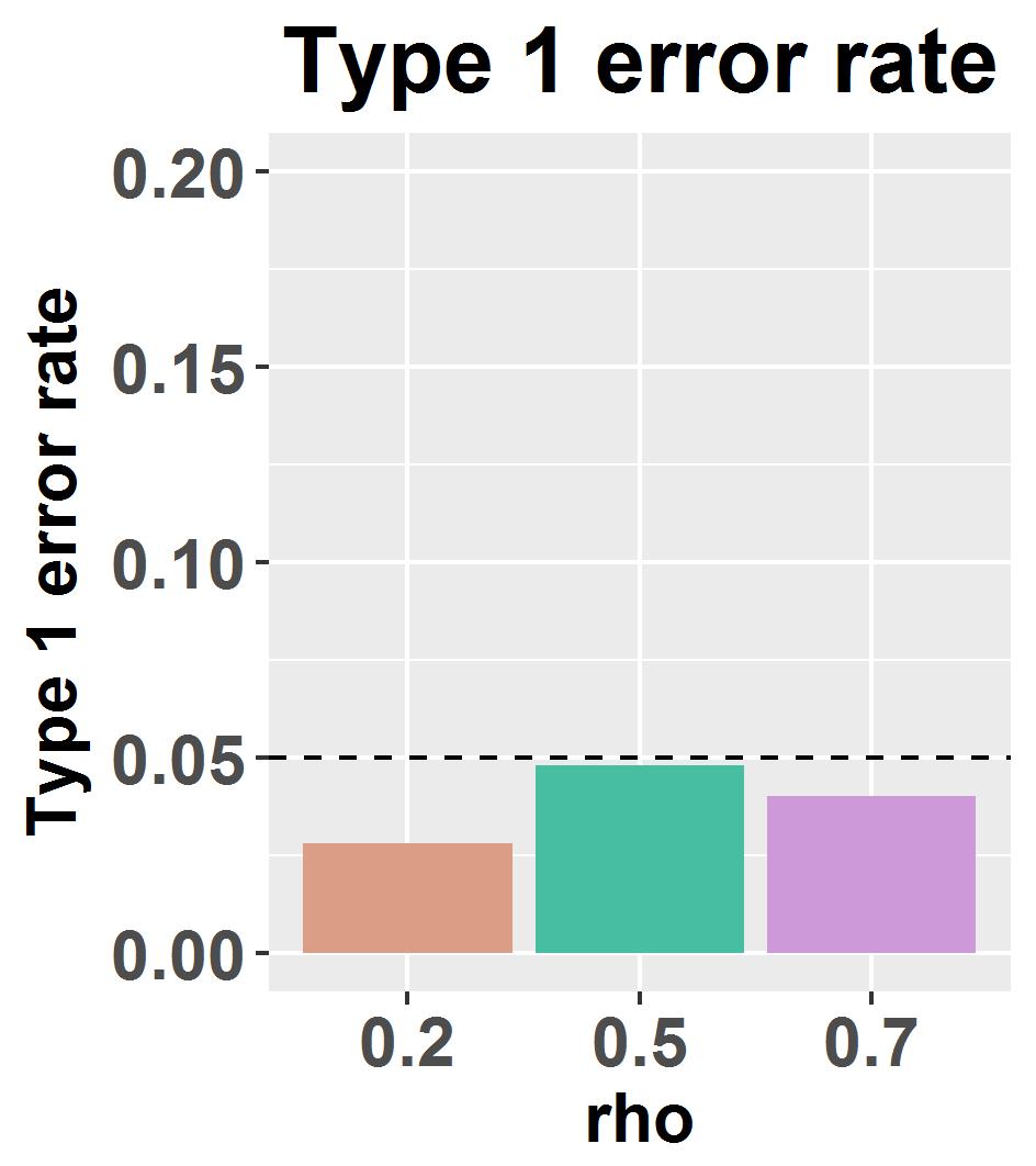
We evaluated the type 1 error and power of the hypothesis test for pleiotropy. As shown in Figure S19 in the supplementary document, the power increases with the ascending trend of pleiotropy ($g$) and the similar performance among different $\rho$ for both the quantitative and binary traits can be found there. Type 1 error for different choice of $\rho$ is shown in Figure S20 in the supplementary document. One can find that type 1 error is a little conservative for both the quantitative and binary traits.

Since WTCCC used shared controls among seven diseases and samples in the control group were from two cohorts (the 1958 British Birth Cohort (58C) and UK Blood Services (UKBS)), we used one control cohort for RA and the other for T1D. After quality control filtering, 240,101 SNPs in 1,812 cases from RA, 1,932 cases from T1D, and 2,897 controls from two data sets were retained for the following analysis. First, we conducted the analysis for 58C controls with RA and UKBS controls with T1D using LPG and BVSR. The prioritization results are shown in Figure 3 in addition to a complete list of findings in Table 1, in which the cut off point is 0.2 in terms of lfdr. As shown in Table 2, LPG identified slightly more SNPs than these from BVSR. The estimated proportions were $\hat{\alpha}_{00}=0.9999$, $\hat{\alpha}_{01}=1.488\times 10^{-10}$, $\hat{\alpha}_{10}=1.499\times 10^{-18}$, $\hat{\alpha}_{11}=5.209\times 10^{-05}$ and $p$-value for the pleiotropy test was $1.68\times 10^{-17}$ suggesting the existence of pleiotropy between RA and T1D. In summary, leveraging the pleiotropic effects enabled LPG to identify more risk SNPs over the single-trait analysis (BVSR). For example, rs6679677 within PTPN22 gene and rs9272346 within MHC region exhibited higher significance using the joint analysis of LPG, which was previously reported (Burton et al., 2007). In addition, T1D-associated SNP rs9272346 was also found to be associated with RA in Pakistani patients (Kiani et al., 2015), rs10484565 within TAP2 gene was shown to confer risk enriched in the RA group (Lee et al., 2008), and rs241427 near TAP1/TAP2 was shown to have relatively strong associations in the collective interaction analysis of RA and T1D (Woo et al., 2017). We also evaluated the prediction performance using RA and T1D. Specifically, we quantitatively assessed the performance of risk prediction using 10-fold cross validation. The prediction accuracy of both LPG and BVSR is shown in Table 2. Clearly, it shows that the joint analysis of RA and T1D consistently outperformed the separate analysis of each study in terms of prediction accuracy, which improved from 62.8$\%$ to 64.4$\%$ for RA and from 76.7$\%$ to 78.3$\%$ for T1D as shown in Table 2. It took around 7 minutes to finish the joint analysis as shown in Table S3 in the supplementary document. To demonstrate the robustness of our LPG, we switched the control cohorts for RA and T1D and conducted the same analysis again and the results were similar.

After the basic quality control filtering as described above, 240,393 SNPs remained in 1,675 cases from CD, 1,932 cases from T1D, and 2,895 controls from two data sets were used for analysis. After excluding the MHC region SNPs, leaving us a total of 239,931 SNPs, we performed the same four comparisons. Here we are presenting the one with 58C controls for CD and UKBS controls for T1D by excluding MHC region. The Manhattan plots are shown in Figure S33 and all SNP findings are shown in Table S17 in the supplementary document, where the threshold for lfdr is set to 0.2. Obviously, the LPG identified slightly more risk SNPs than these from two-groups model (BVSR). The estimated proportions were $\hat{\alpha}_{00}=0.9999$, $\hat{\alpha}_{01}=4.477\times 10^{-5}$, $\hat{\alpha}_{10}=2.058\times 10^{-9}$ and $\hat{\alpha}_{11}=3.898\times 10^{-05}$, and $p$-values for the pleiotropy test was $2.96\times 10^{-2}$ suggesting the existence of pleiotropy between CD and T1D. For example, rs11805303 in the IL23R gene was identified to be strongly associated with CD, which was previously reported (Buzdugan et al., 2016). Another intergenic SNP rs2542151 identified by LPG was also reported to be significantly associated with CD (Parkes et al., 2007). Besides, rs17234657 on chromosome 5 was identified to be associated with CD by both LPG and BVSR, which was also previously reported in (Burton et al., 2007). The prediction performance of both LPG and BVSR is shown in Table S16 in the supplementary document. The results demonstrate that the prediction of the jointly analysis of CD and T1D was slightly better than the separate analysis of each study, which improved from 58.1$\%$ to 58.7$\%$ for CD and from 60.1$\%$ to 60.3$\%$ for T1D. The rest results of other comparisons are detailed in the supplementary document and they were similar to the one we presented here.

References

• Bishop [2006] Christopher M Bishop. Pattern recognition. Machine Learning, 128:1–58, 2006.
• Böhning [1992] Dankmar Böhning. Multinomial logistic regression algorithm. Annals of the Institute of Statistical Mathematics, 44(1):197–200, 1992.
• Burton et al. [2007] Paul R Burton, David G Clayton, Lon R Cardon, Nick Craddock, Panos Deloukas, Audrey Duncanson, Dominic P Kwiatkowski, Mark I McCarthy, Willem H Ouwehand, Nilesh J Samani, et al. Genome-wide association study of 14,000 cases of seven common diseases and 3,000 shared controls. Nature, 447(7145):661–678, 2007.
• Buzdugan et al. [2016] Laura Buzdugan, Markus Kalisch, Arcadi Navarro, Daniel Schunk, Ernst Fehr, and Peter Bühlmann. Assessing statistical significance in multivariable genome wide association analysis. Bioinformatics, 32(13):1990–2000, 2016.
• Cotsapas et al. [2011] Chris Cotsapas, Benjamin F Voight, Elizabeth Rossin, Kasper Lage, Benjamin M Neale, Chris Wallace, Gonçalo R Abecasis, Jeffrey C Barrett, Timothy Behrens, Judy Cho, et al. Pervasive sharing of genetic effects in autoimmune disease. PLoS genetics, 7(8):e1002254, 2011.
• Dai et al. [2017] Mingwei Dai, Jingsi Ming, Mingxuan Cai, Jin Liu, Can Yang, Xiang Wan, and Zongben Xu. Igess: a statistical approach to integrating individual-level genotype data and summary statistics in genome-wide association studies. Bioinformatics, 2017.
• Efron [2012] Bradley Efron. Large-scale inference: empirical Bayes methods for estimation, testing, and prediction, volume 1. Cambridge University Press, 2012.
• Efron et al. [2008] Bradley Efron et al. Microarrays, empirical bayes and the two-groups model. Statistical science, 23(1):1–22, 2008.
• Fogarty et al. [2005] James Fogarty, Ryan S Baker, and Scott E Hudson. Case studies in the use of roc curve analysis for sensor-based estimates in human computer interaction. In Proceedings of Graphics Interface 2005, pages 129–136. Canadian Human-Computer Communications Society, 2005.
• Friedman et al. [2001] Jerome Friedman, Trevor Hastie, and Robert Tibshirani. The elements of statistical learning, volume 1. Springer series in statistics Springer, Berlin, 2001.
• Friedman et al. [2010] Jerome Friedman, Trevor Hastie, and Rob Tibshirani. Regularization paths for generalized linear models via coordinate descent. Journal of statistical software, 33(1):1, 2010.
• Guan and Stephens [2011] Yongtao Guan and Matthew Stephens. Bayesian variable selection regression for genome-wide association studies and other large-scale problems. The Annals of Applied Statistics, pages 1780–1815, 2011.
• Jordan et al. [1999] Michael I Jordan, Zoubin Ghahramani, Tommi S Jaakkola, and Lawrence K Saul. An introduction to variational methods for graphical models. Machine learning, 37(2):183–233, 1999.
• Kiani et al. [2015] Aysha Karim Kiani, Sidrah Jahngir, Peter John, Attya Bhatti, Asima Zia, Xingbin Wang, F Yesim Demirci, and M Ilyas Kamboh. Genetic link of type 1 diabetes susceptibility loci with rheumatoid arthritis in pakistani patients. Immunogenetics, 67(5-6):277–282, 2015.
• Kraja et al. [2014] Aldi T Kraja, Daniel I Chasman, Kari E North, Alexander P Reiner, Lisa R Yanek, Tuomas O Kilpeläinen, Jennifer A Smith, Abbas Dehghan, Josée Dupuis, Andrew D Johnson, et al. Pleiotropic genes for metabolic syndrome and inflammation. Molecular genetics and metabolism, 112(4):317–338, 2014.
• Kuo and Mallick [1998] Lynn Kuo and Bani Mallick. Variable selection for regression models. Sankhyā: The Indian Journal of Statistics, Series B, pages 65–81, 1998.
• Lee et al. [2008] Hye-Soon Lee, Annette T Lee, Lindsey A Criswell, Michael F Seldin, Christopher I Amos, John P Carulli, Cristina Navarrete, Elaine F Remmers, Daniel L Kastner, Robert M Plenge, et al. Several regions in the major histocompatibility complex confer risk for anti-ccp-antibody positive rheumatoid arthritis, independent of the drb1 locus. MOLECULAR MEDICINE-CAMBRIDGE MA THEN NEW YORK-, 14(5/6):293, 2008.
• Lee et al. [2011] Sang Hong Lee, Naomi R Wray, Michael E Goddard, and Peter M Visscher. Estimating missing heritability for disease from genome-wide association studies. The American Journal of Human Genetics, 88(3):294–305, 2011.
• Liu et al. [2016] Jin Liu, Can Yang, Xingjie Shi, Cong Li, Jian Huang, Hongyu Zhao, and Shuangge Ma. Analyzing association mapping in pedigree-based gwas using a penalized multitrait mixed model. Genetic epidemiology, 40(5):382–393, 2016.
• Manolio et al. [2009] Teri A Manolio, Francis S Collins, Nancy J Cox, David B Goldstein, Lucia A Hindorff, David J Hunter, Mark I McCarthy, Erin M Ramos, Lon R Cardon, Aravinda Chakravarti, et al. Finding the missing heritability of complex diseases. Nature, 461(7265):747, 2009.
• Newton et al. [2004] Michael A Newton, Amine Noueiry, Deepayan Sarkar, and Paul Ahlquist. Detecting differential gene expression with a semiparametric hierarchical mixture method. Biostatistics, 5(2):155–176, 2004.
• Opper and Saad [2001] Manfred Opper and David Saad. Advanced mean field methods: Theory and practice. MIT press, 2001.
• Parkes et al. [2007] Miles Parkes, Jeffrey C Barrett, Natalie Prescott, Mark Tremelling, Carl A Anderson, Sheila A Fisher, Roland G Roberts, Elaine R Nimmo, Fraser R Cummings, Dianne Soars, et al. Sequence variants in the autophagy gene irgm and multiple other replicating loci contribute to crohn disease susceptibility. Nature genetics, 39(7):830, 2007.
• Purcell et al. [2007] Shaun Purcell, Benjamin Neale, Kathe Todd-Brown, Lori Thomas, Manuel AR Ferreira, David Bender, Julian Maller, Pamela Sklar, Paul IW De Bakker, Mark J Daly, et al. Plink: a tool set for whole-genome association and population-based linkage analyses. The American Journal of Human Genetics, 81(3):559–575, 2007.
• Solovieff et al. [2013] Nadia Solovieff, Chris Cotsapas, Phil H Lee, Shaun M Purcell, and Jordan W Smoller. Pleiotropy in complex traits: challenges and strategies. Nature reviews. Genetics, 14(7):483, 2013.
• Wagner and Zhang [2011] Günter P Wagner and Jianzhi Zhang. The pleiotropic structure of the genotype–phenotype map: the evolvability of complex organisms. Nature Reviews Genetics, 12(3):204–213, 2011.
• Wang et al. [2015] Qian Wang, Can Yang, Joel Gelernter, and Hongyu Zhao. Pervasive pleiotropy between psychiatric disorders and immune disorders revealed by integrative analysis of multiple gwas. Human genetics, 134(11-12):1195–1209, 2015.
• Woo et al. [2017] Hyung Jun Woo, Chenggang Yu, and Jaques Reifman. Collective genetic interaction effects and the role of antigen-presenting cells in autoimmune diseases. PLOS ONE, 12(1):e0169918, 2017.
• Yang et al. [2011] Jian Yang, S Hong Lee, Michael E Goddard, and Peter M Visscher. Gcta: a tool for genome-wide complex trait analysis. The American Journal of Human Genetics, 88(1):76–82, 2011.
• Zhou and Stephens [2014] Xiang Zhou and Matthew Stephens. Efficient multivariate linear mixed model algorithms for genome-wide association studies. Nature methods, 11(4):407–409, 2014.
Supplementary information for “FGP: a four-group probabilistic model to account for pleiotropic effects for multiple GWAS”
1 Simulation studies: Quantitative trait
For the quantitative trait, we conducted simulation studies to evaluate the performance of FGP with its alternative, i.e. BVSR and Lasso. We first evaluated their performance of the identification of risk variants using AUC, statistical power, and FDR. Note that we can only evaluate AUC for Lasso and FDR was controlled at 0.2. We then evaluated the prediction performance by measuring the Pearson’s correlation between observed phenotypic values and estimated phenotypic values in a testing set for all three methods. The number of replicates in simulation studies was 50 for all settings. The results are provided in Figure S1-S9 and they demonstrate that the performance of FGP gradually gets better as the pleiotropic effects become stronger.
h2h^{2}=0.3 h2h^{2}=0.4 h2h^{2}=0.5
ρ\rho=0.2 Figure S  11 Figure S  44 Figure S  77
ρ\rho=0.5 Figure S  22 Figure S  55 Figure S  88
ρ\rho=0.7 Figure S  33 Figure S  66 Figure S  99
Table S1: A table of simulation settings for quantitative trait scenario, Figure S means Supplementary Figure
ρ\rho=0.2 Figure S   1010 Figure S   1313 Figure S   1616
ρ\rho=0.5 Figure S   1111 Figure S   1414 Figure S   1717
ρ\rho=0.7 Figure S   1212 Figure S   1515 Figure S   1818
Table S2: A table of simulation settings for binary trait scenario, Figure S means Supplementary Figure
Refer to caption
Figure S1: Comparison of FGP (VB joint), BVSR (VB separate), and Lasso for different choice gg ranging from 0 to 1 for quantitative trait. Panels from top to bottom are AUC, FDR, Power and Prediction, respectively. The parameter setting of the model is : pp = 20,000, n1=n2n_{1}=n_{2} = 3000, h2h^{2} = 0.3, ρ=0.2\rho=0.2, α1\alpha_{1} = 0.005.
Figure S2: Comparison of FGP (VB joint), BVSR (VB separate), and Lasso for different choice gg ranging from 0 to 1 for quantitative trait. Panels from top to bottom are AUC, FDR, Power and Prediction, respectively. The parameter setting of the model is : pp = 20,000, n1=n2n_{1}=n_{2} = 3000, h2h^{2} = 0.3, ρ=0.5\rho=0.5, α1\alpha_{1} = 0.005.
Figure S3: Comparison of FGP (VB joint), BVSR (VB separate), and Lasso for different choice gg ranging from 0 to 1 for quantitative trait. Panels from top to bottom are AUC, FDR, Power and Prediction, respectively. The parameter setting of the model is : pp = 20,000, n1=n2n_{1}=n_{2} = 3000, h2h^{2} = 0.3, ρ=0.7\rho=0.7, α1\alpha_{1} = 0.005.
Figure S4: Comparison of FGP (VB joint), BVSR (VB separate), and Lasso for different choice gg ranging from 0 to 1 for quantitative trait. Panels from top to bottom are AUC, FDR, Power and Prediction, respectively. The parameter setting of the model is : pp = 20,000, n1=n2n_{1}=n_{2} = 3000, h2h^{2} = 0.4, ρ=0.2\rho=0.2, α1\alpha_{1} = 0.005.
Figure S5: Comparison of FGP (VB joint), BVSR (VB separate), and Lasso for different choice gg ranging from 0 to 1 for quantitative trait. Panels from top to bottom are AUC, FDR, Power and Prediction, respectively. The parameter setting of the model is : pp = 20, 000, n1=n2n_{1}=n_{2} = 3000, h2h^{2} = 0.4, ρ=0.5\rho=0.5, α1\alpha_{1} = 0.005.
Figure S6: Comparison of FGP (VB joint), BVSR (VB separate), and Lasso for different choice gg ranging from 0 to 1 for quantitative trait. Panels from top to bottom are AUC, FDR, Power and Prediction, respectively. The parameter setting of the model is : pp = 20,000, n1=n2n_{1}=n_{2} = 3000, h2h^{2} = 0.4, ρ=0.7\rho=0.7, α1\alpha_{1} = 0.005.
Figure S7: Comparison of FGP (VB joint), BVSR (VB separate), and Lasso for different choice gg ranging from 0 to 1 for quantitative trait. Panels from top to bottom are AUC, FDR, Power and Prediction, respectively. The parameter setting of the model is : pp = 20,000, n1=n2n_{1}=n_{2} = 3000, h2h^{2} = 0.5, ρ=0.2\rho=0.2, α1\alpha_{1} = 0.005.
Figure S8: Comparison of FGP (VB joint), BVSR (VB separate), and Lasso for different choice gg ranging from 0 to 1 for quantitative trait. Panels from top to bottom are AUC, FDR, Power and Prediction, respectively. The parameter setting of the model is : pp = 20,000, n1=n2n_{1}=n_{2} = 3000, h2h^{2} = 0.5, ρ=0.5\rho=0.5, α1\alpha_{1} = 0.005.
Figure S9: Comparison of FGP (VB joint), BVSR (VB separate), and Lasso for different choice gg ranging from 0 to 1 for quantitative trait. Panels from top to bottom are AUC, FDR, Power and Prediction, respectively. The parameter setting of the model is : pp = 20,000, n1=n2n_{1}=n_{2} = 3000, h2h^{2} = 0.5, ρ=0.7\rho=0.7, α1\alpha_{1} = 0.005.
2 Simulation studies: Binary trait
For the binary trait in case-control studies,we conducted simulation studies to evaluate the performance of FGP with its alternative, i.e. BVSR and Lasso. We first evaluated their performance of the identification of risk variants using AUC, statistical power, and FDR. Note that we can only evaluate AUC for Lasso and FDR was controlled at 0.2. Thirdly, we measure the proportion of true risk SNPs discovered by Power. We then evaluated the prediction performance in a testing set using AUC as described in Section 3.2 for all three methods The results are provided in Supplementary Figure S10-S18 and they demonstrate that the performance of FGP gradually gets better as the pleiotropic effects become stronger.
Figure S10: Comparison of FGP (VB joint), BVSR (VB separate), and Lasso with different gg ranging from 0 to 1 for binary trait. Panels from top to bottom are AUC, FDR, Power and Prediction, respectively. The parameter setting of the model is : pp = 20,000, n1=n2n_{1}=n_{2} = 3000, h2h^{2} = 0.3, ρ=0.2\rho=0.2, α1\alpha_{1} = 0.0025.
Figure S11: Comparison of FGP (VB joint), BVSR (VB separate), and Lasso with different gg ranging from 0 to 1 for binary trait. Panels from top to bottom are AUC, FDR, Power and Prediction, respectively. The parameter setting of the model is : pp = 20,000, n1=n2n_{1}=n_{2} = 3000, h2h^{2} = 0.3, ρ=0.5\rho=0.5, α1\alpha_{1} = 0.0025.
Figure S12: Comparison of FGP (VB joint), BVSR (VB separate), and Lasso with different gg ranging from 0 to 1 for binary trait. Panels from top to bottom are AUC, FDR, Power and Prediction, respectively. The parameter setting of the model is : pp = 20,000, n1=n2n_{1}=n_{2} = 3000, h2h^{2} = 0.3, ρ=0.7\rho=0.7, α1\alpha_{1} = 0.0025.
Figure S13: Comparison of FGP (VB joint), BVSR (VB separate), and Lasso with different gg ranging from 0 to 1 for binary trait. Panels from top to bottom are AUC, FDR, Power and Prediction, respectively. The parameter setting of the model is : pp = 20,000, n1=n2n_{1}=n_{2} = 3000, h2h^{2} = 0.4, ρ=0.2\rho=0.2, α1\alpha_{1} = 0.0025.
Figure S14: Comparison of FGP (VB joint), BVSR (VB separate), and Lasso with different gg ranging from 0 to 1 for binary trait. Panels from top to bottom are AUC, FDR, Power and Prediction, respectively. The parameter setting of the model is : pp = 20,000, n1=n2n_{1}=n_{2} = 3000, h2h^{2} = 0.4, ρ=0.5\rho=0.5, α1\alpha_{1} = 0.0025.
Figure S15: Comparison of FGP (VB joint), BVSR (VB separate), and Lasso with different gg ranging from 0 to 1 for binary trait. Panels from top to bottom are AUC, FDR, Power and Prediction, respectively. The parameter setting of the model is : pp = 20,000, n1=n2n_{1}=n_{2} = 3000, h2h^{2} = 0.4, ρ=0.7\rho=0.7, α1\alpha_{1} = 0.0025.
Figure S16: Comparison of FGP (VB joint), BVSR (VB separate), and Lasso with different gg ranging from 0 to 1 for binary trait. Panels from top to bottom are AUC, FDR, Power and Prediction, respectively. The parameter setting of the model is : pp = 20,000, n1=n2n_{1}=n_{2} = 3000, h2h^{2} = 0.5, ρ=0.2\rho=0.2, α1\alpha_{1} = 0.0025.
Figure S17: Comparison of FGP (VB joint), BVSR (VB separate), and Lasso with different gg ranging from 0 to 1 for binary trait. Panels from top to bottom are AUC, FDR, Power and Prediction, respectively. The parameter setting of the model is : pp = 20,000, n1=n2n_{1}=n_{2} = 3000, h2h^{2} = 0.5, ρ=0.5\rho=0.5, α1\alpha_{1} = 0.0025.
Figure S18: Comparison of FGP (VB joint), BVSR (VB separate), and Lasso with different gg ranging from 0 to 1 for binary trait. Panels from top to bottom are AUC, FDR, Power and Prediction, respectively. The parameter setting of the model is : pp = 20,000, n1=n2n_{1}=n_{2} = 3000, h2h^{2} = 0.5, ρ=0.7\rho=0.7, α1\alpha_{1} = 0.0025.
Figure S19: Power of pleiotropy test for both quantitative (left panel) and binary (right panel) trait. ρ\rho is chosen to be 0.2, 0.5, 0.7, h2h_{2} is 0.5 and the pleiotropy parameter gg is controlled at 0.1, 0.2, 0.3. The number of replicates is 100.
Figure S20: Type I error of pleiotropy test for quantitative (left panel) and binary (right panel) trait. ρ\rho is chosen to be 0.2, 0.5, 0.7 and h2h_{2} is 0.5. The number of replicates is 500.
3 Real data analysis
iter-sep1 time-sep1(s) iter-sep2 time-sep2(s) iter-joint time-joint(s)
RA-T1D-inMHC 69 271.70 27 139.88 69 713.53
T1D-RA-inMHC 29 72.98 66 167.67 75 451.86
RA-T1D-exMHC 160 540.37 100 403.49 175 1736.89
T1D-RA-exMHC 106 374.78 134 522.26 178 1441.98
CD-T1D-inMHC 177 427.43 27 73.75 305 1778.91
T1D-CD-inMHC 27 128.62 183 583.80 237 2187.62
CD-T1D-exMHC 177 372.41 101 263.57 217 1170.94
T1D-CD-exMHC 107 319.80 183 422.41 220 1366.07
Table S3: Summary of real data analysis, inMHC and exMHC mean SNPs include and exclude MHC region, respectively, iter-sep1 and iter-sep2 mean iterations of separate analysis using BVSR for first and second study, respectively, iter-joint means iterations of joint analysis using FGP, time-sep1 and time-sep2 mean time of separate analysis using BVSR for first and second study, respectively, time-joint means time of joint analysis
3.1 Comparison of FGP and BVSR for the data consisting of 58C controls with T1D and UKBS controls with RA
Figure S21: For the data consisting of 58C controls with T1D and UKBS controls with RA, manhattan plots of separate analysis using BVSR and joint analysis using FGP.
Figure S22: For the data consisting of 58C controls with T1D and UKBS controls with RA, prediction performance of separate analysis using BVSR and joint analysis using FGP.
Data number of hits prediction accuracy(AUC)
1 Rheumatoid arthritis(RA)joint 11 63.2%(2.5%)
2 Type 1 diabetes(T1D)joint 11 75.7%(2.2%)
3 Rheumatoid arthritis(RA)separate 3 60.9%(2.8%)
4 Type 1 diabetes(T1D)separate 10 75.2%(2.8%)
Table S4: For the data consisting of 58C controls with T1D and UKBS controls with RA, summary of separate and joint analysis of RA and T1D
snp chr position sep RA(fdr) sep T1D(fdr) joi RA(fdr) joi T1D(fdr)
1 rs6679677 1 114303808 2.5e-11* 0e+00* 0e+00* 0e+00*
2 rs13200022 6 31098957 1e+00 5.77e-06* 1.82e-09* 1.37e-14*
3 rs3130484 6 31715882 1e+00 8.35e-06* 1e+00 1e+00
4 rs2075800 6 31777946 6.91e-14* 1e+00 1e+00 1e+00
5 rs550513 6 31920687 9.88e-01 1e+00 6.3e-06* 6.3e-06*
6 rs3130287 6 32050544 1e+00 0e+00* 2.79e-08* 1.11e-16*
7 rs17421624 6 32066177 1e+00 1e+00 2.22e-16* 1.11e-16*
8 rs9272346 6 32604372 1.14e-03* 0e+00* 1.03e-11* 0e+00*
9 rs2070121 6 32781554 1e+00 1.22e-11* 2.22e-16* 0e+00*
10 rs10484565 6 32795032 9.97e-01 1.55e-15* 0e+00* 0e+00*
11 rs241427 6 32804414 1e+00 1.1e-08* 1.24e-09* 1.28e-10*
12 rs12529313 6 32817130 1e+00 7.3e-08* 3.05e-04* 3.05e-04*
13 rs11171739 12 56470625 1e+00 2.61e-04* 1.63e-03* 1.63e-03*
Table S5: For the data consisting of 58C controls with T1D and UKBS controls with RA, list of SNPs of two modes: separate analysis and joint analysis. * denotes the local fdr <0.2, sep means separate, joi means joint.
3.2 Comparison of FGP and BVSR for the data consisting of 58C controls with T1D and UKBS controls with RA exclude MHC region
Figure S23: For the data consisting of 58C controls with T1D and UKBS controls with RA exclude MHC region SNPs, manhattan plots of separate analysis using BVSR and joint analysis using FGP.
Figure S24: For the data consisting of 58C controls with T1D and UKBS controls with RA exclude MHC region SNPs, prediction performance of separate analysis using BVSR and joint analysis using FGP.
1 Rheumatoid arthritis(RA)joint 2 56.7%(2.9%)
2 Type 1 diabetes(T1D)joint 3 58.4%(2.8%)
3 Rheumatoid arthritis(RA)separate 1 52.5%(2.1%)
4 Type 1 diabetes(T1D)separate 3 58.8%(2.9%)
Table S6: For the data consisting of 58C controls with T1D and UKBS controls with RA exclude MHC region, summary of separate and joint analysis of RA and T1D
1 rs6679677 1 114303808 6.61e-11* 6.66e-15* 6.66e-16* 1.11e-16*
2 rs11171739 12 56470625 1e+00 5.1e-03* 6.42e-01 1.48e-02*
3 rs17696736 12 112486818 1e+00 1.26e-03* 1.03e-01* 4.85e-04*
Table S7: For the data consisting of 58C controls with T1D and UKBS controls with RA exclude MHC region, list of SNPs of two modes: separate analysis and joint analysis. * denotes the local fdr <0.2, sep means separate, joi means joint.
3.3 Comparison of FGP and BVSR for the data consisting of 58C controls with RA and UKBS controls with T1D exclude MHC region
Figure S25: For the data consisting of 58C controls with RA and UKBS controls with T1D exclude MHC region SNPs, manhattan plots of separate analysis using BVSR and joint analysis using FGP.
Figure S26: For the data consisting of 58C controls with RA and UKBS controls with T1D exclude MHC region SNPs, prediction performance of separate analysis using BVSR and joint analysis using FGP.
1 Type 1 diabetes(T1D)joint 3 59.1%(2.1%)
2 Rheumatoid arthritis(RA)joint 1 56.7%(2.6%)
3 Type 1 diabetes(T1D)separate 3 59.8%(2.2%)
4 Rheumatoid arthritis(RA)separate 1 56.4%(2.7%)
Table S8: For the data consisting of 58C controls with RA and UKBS controls with T1D exclude MHC region, summary of separate and joint analysis of T1D and RA
snp chr position sep T1D(fdr) sep RA(fdr) joi T1D(fdr) joi RA(fdr)
1 rs6679677 1 114303808 3.78e-13* 7.34e-13* 0e+00* 0e+00*
2 rs2292239 12 56482180 1.65e-02* 1e+00 2.82e-02* 8.81e-01
3 rs17696736 12 112486818 4.95e-06* 1e+00 5.5e-06* 5.96e-01
Table S9: For the data consisting of 58C controls with RA and UKBS controls with T1D exclude MHC region, list of SNPs of two modes: separate analysis and joint analysis. * denotes the local fdr <0.2, sep means separate, joi means joint.
3.4 Comparison of FGP and BVSR for the data consisting of 58C controls with T1D and UKBS controls with CD
Figure S27: For the data consisting of 58C controls with T1D and UKBS controls with CD, manhattan plots of separate analysis using BVSR and joint analysis using FGP.
Figure S28: For the data consisting of 58C controls with T1D and UKBS controls with CD, prediction performance of separate analysis using BVSR and joint analysis using FGP.
1 Crohn’s disease(CD)joint 3 57.6%(3.7%)
2 Type 1 diabetes(T1D)joint 10 75.6%(2.8%)
3 Crohn’s disease(CD)separate 3 57.4%(3.6%)
4 Type 1 diabetes(T1D)separate 10 75.7%(2.8%)
Table S10: For the data consisting of 58C controls with T1D and UKBS controls with CD, summary of separate and joint analysis of CD and T1D
snp chr position sep CD(fdr) sep T1D(fdr) joi CD(fdr) joi T1D(fdr)
1 rs6679677 1 114303808 1e+00 0e+00* 9.98e-01 0e+00*
2 rs10210302 2 234158839 1.1e-01* 1e+00 1.1e-01* 9.99e-01
3 rs9292777 5 40437948 1.45e-04* 1e+00 1.45e-04* 1e+00
4 rs13200022 6 31098957 1e+00 5.58e-06* 1e+00 5.57e-06*
5 rs3130484 6 31715882 1e+00 2.06e-05* 1e+00 2.06e-05*
6 rs3130287 6 32050544 1e+00 0e+00* 9.98e-01 0e+00*
7 rs9272346 6 32604372 1e+00 0e+00* 9.98e-01 1.11e-16*
8 rs2070121 6 32781554 1e+00 1.23e-11* 1e+00 1.21e-11*
9 rs10484565 6 32795032 1e+00 1.55e-15* 1e+00 1.44e-15*
10 rs241427 6 32804414 1e+00 1.29e-08* 1e+00 1.29e-08*
11 rs12529313 6 32817130 1e+00 7.63e-08* 1e+00 7.59e-08*
12 rs11171739 12 56470625 1e+00 2.61e-04* 1e+00 2.61e-04*
13 rs2066843 16 50745199 8.8e-06* 1e+00 8.81e-06* 1e+00
Table S11: For the data consisting of 58C controls with T1D and UKBS controls with CD, list of SNPs of two modes: separate analysis and joint analysis. * denotes the local fdr <0.2, sep means separate, joi means joint.
3.5 Comparison of FGP and BVSR for the data consisting of 58C controls with CD and UKBS controls with T1D
Figure S29: For the data consisting of 58C controls with CD and UKBS controls with T1D, manhattan plots of separate analysis using BVSR and joint analysis using FGP.
Figure S30: For the data consisting of 58C controls with CD and UKBS controls with T1D, prediction performance of separate analysis using BVSR and joint analysis using FGP.
1 Type 1 diabetes(T1D)joint 12 76.9%(3.3%)
2 Crohn’s disease(CD)joint 4 57.9%(4.5%)
3 Type 1 diabetes(T1D)separate 10 76.8%(3.2%)
4 Crohn’s disease(CD)separate 3 57.9%(4.7%)
Table S12: For the data consisting of 58C controls with CD and UKBS controls with T1D, summary of separate and joint analysis of T1D and CD
snp chr position sep T1D(fdr) sep CD(fdr) joi T1D(fdr) joi CD(fdr)
1 rs11805303 1 67675516 1e+00 2.2e-06* 9.45e-01 3.58e-06*
2 rs6679677 1 114303808 0e+00* 1e+00 0e+00* 6.02e-01
3 rs6752107 2 234161448 1e+00 9.06e-05* 9.58e-01 1.81e-04*
4 rs17234657 5 40401509 1e+00 4.14e-02* 9.61e-01 4.96e-02*
5 rs13200022 6 31098957 9.26e-12* 1e+00 0e+00* 8.11e-01
6 rs550513 6 31920687 9.98e-01 1e+00 1.73e-05* 8.28e-01
7 rs3130287 6 32050544 0e+00* 1e+00 -2.22e-16* 5.14e-01
8 rs17421624 6 32066177 9.7e-01 1e+00 1.27e-08* 8.66e-01
9 rs9272346 6 32604372 0e+00* 1e+00 0e+00* 8.94e-01
10 rs2070121 6 32781554 0e+00* 1e+00 6.66e-16* 7.21e-01
11 rs10484565 6 32795032 0e+00* 1e+00 1.11e-16* 8.59e-01
12 rs241427 6 32804414 1.51e-07* 1e+00 1.34e-04* 8.93e-01
13 rs12529313 6 32817130 8.28e-05* 1e+00 9.84e-01 9.98e-01
14 rs10759987 9 121364134 2.15e-03* 1e+00 2.84e-03* 8.92e-01
15 rs17696736 12 112486818 4.87e-05* 1e+00 2.45e-06* 4.93e-01
16 rs2542151 18 12779947 1e+00 8.09e-01 4.59e-02* 2.61e-02*
Table S13: For the data consisting of 58C controls with CD and UKBS controls with T1D, list of SNPs of two modes: separate analysis and joint analysis. * denotes the local fdr <0.2, sep means separate, joi means joint.
3.6 Comparison of FGP and BVSR for the data consisting of 58C controls with T1D and UKBS controls with CD exclude MHC region
Figure S31: For the data consisting of 58C controls with T1D and UKBS controls with CD exclude MHC region SNPs, manhattan plots of separate analysis using BVSR and joint analysis using FGP.
Figure S32: For the data consisting of 58C controls with T1D and UKBS controls with CD exclude MHC region SNPs, prediction performance of separate analysis using BVSR and joint analysis using FGP.
1 Crohn’s disease(CD)joint 8 58.6%(4.2%)
2 Type 1 diabetes(T1D)joint 4 58.6%(3%)
3 Crohn’s disease(CD)separate 3 57.4%(4.4%)
4 Type 1 diabetes(T1D)separate 3 58.5%(2.8%)
Table S14: For the data consisting of 58C controls with T1D and UKBS controls with CD exclude MHC region, summary of separate and joint analysis of CD and T1D
1 rs4655679 1 67599657 3.11e-01 1e+00 1.5e-01* 6.45e-01
2 rs6679677 1 114303808 1e+00 6.44e-15* 7.53e-08* 3.33e-15*
3 rs10210302 2 234158839 1.09e-01* 1e+00 6.33e-02* 4.75e-01
4 rs9292777 5 40437948 1.49e-04* 1e+00 2.24e-04* 7.42e-01
5 rs11171739 12 56470625 1e+00 5.13e-03* 1.29e-02* 1.29e-02*
6 rs17696736 12 112486818 1e+00 1.24e-03* 4.76e-05* 4.76e-05*
7 rs2066843 16 50745199 8.5e-06* 1e+00 1.21e-05* 8.3e-01
8 rs2542151 18 12779947 9.69e-01 9.97e-01 3.28e-02* 3.65e-02*
Table S15: For the data consisting of 58C controls with T1D and UKBS controls with CD exclude MHC region, list of SNPs of two modes: separate analysis and joint analysis. * denotes the local fdr <0.2, sep means separate, joi means joint.
3.7 Comparison of FGP and BVSR for the data consisting of 58C controls with CD and UKBS controls with T1D exclude MHC region
Figure S33: For the data consisting of 58C controls with CD and UKBS controls with T1D exclude MHC region SNPs, manhattan plots of separate analysis using BVSR and joint analysis using FGP.
Figure S34: For the data consisting of 58C controls with CD and UKBS controls with T1D exclude MHC region SNPs, prediction performance of separate analysis using BVSR and joint analysis using FGP.
1 Type 1 diabetes(T1D)joint 4 60.3%(2%)
2 Crohn’s disease(CD)joint 7 58.7%(4.1%)
3 Type 1 diabetes(T1D)separate 4 60.1%(2.3%)
4 Crohn’s disease(CD)separate 3 58.1%(4.4%)
Table S16: For the data consisting of 58C controls with CD and UKBS controls with T1D exclude MHC region, summary of separate and joint analysis of T1D and CD
1 rs11805303 1 67675516 1e+00 2.18e-06* 8.17e-01 8.89e-06*
2 rs6679677 1 114303808 3.98e-13* 1e+00 1.44e-13* 2.94e-05*
3 rs6752107 2 234161448 1e+00 9.34e-05* 8.44e-01 2.15e-04*
4 rs17234657 5 40401509 1e+00 4.14e-02* 8.55e-01 7.8e-02*
5 rs10759987 9 121364134 1.88e-01* 1e+00 7.56e-01 7.56e-01
6 rs2292239 12 56482180 1.41e-02* 1e+00 2.27e-02* 2.28e-02*
7 rs17696736 12 112486818 4.17e-06* 1e+00 8.75e-07* 1.6e-05*
8 rs2542151 18 12779947 9.99e-01 8.11e-01 2.49e-02* 1.22e-02*
Table S17: For the data consisting of 58C controls with CD and UKBS controls with T1D exclude MHC region, list of SNPs of two modes: separate analysis and joint analysis. * denotes the local fdr <0.2, sep means separate, joi means joint.
4 Proof detail for Quantitative trait model
To overcome the intractability of marginal likelihood, we derive an efficient algorithm based on variational inference, which makes our model scalable to genome-wide data analysis. The key idea is that we make use of Jensen’s inequality to iteratively obtain an adjustable lower bound on the marginal log likelihood (Jordan et al., 1999). First, we have a lower bound of the logarithm of the marginal likelihood,
logPr(𝐲1,𝐲2|𝐗1,𝐗2;𝜽)=ℒ(q,𝜽)+𝕂𝕃(q||p)\displaystyle\log\mbox{Pr}({\mathbf{y}}_{1},{\mathbf{y}}_{2}|{\mathbf{X}}_{1},{\mathbf{X}}_{2};\bm{\theta})=\mathcal{L}(q,\bm{\theta})+\mathbb{KL}(q||p) (S1)
≥\displaystyle\geq 𝔼q[logPr(𝐲1,𝐲2,𝜷1,𝜷2,𝜸1,𝜸2|𝐗1,𝐗2;𝜽)]−𝔼q[logq(𝜷1,𝜷2,𝜸1,𝜸2)],\displaystyle\mathbb{E}_{q}[\log\mbox{Pr}({\mathbf{y}}_{1},{\mathbf{y}}_{2},\bm{\beta}_{1},\bm{\beta}_{2},\bm{\gamma}_{1},\bm{\gamma}_{2}|{\mathbf{X}}_{1},{\mathbf{X}}_{2};\bm{\theta})]-\mathbb{E}_{q}[\log q(\bm{\beta}_{1},\bm{\beta}_{2},\bm{\gamma}_{1},\bm{\gamma}_{2})],
• Carbonetto et al. [2012] Peter Carbonetto, Matthew Stephens, et al. Scalable variational inference for bayesian variable selection in regression, and its accuracy in genetic association studies. Bayesian analysis, 7(1):73–108, 2012.