Lattice Boltzmann method for semiclassical fluids

The Boltzmann equation [1] with a Bhatnagar, Gross and Krook (BGK) collision term together with the Maxwell-Boltzmann (MB) equilibrium distribution function (EDF) has found widespread use to describe the flow of classical particles. This is because it allows for an efficient numerical implementation, which is well fitted to perform simulations in complex geometries such as in porous media [2]. This is the lattice Boltzmann method (LBM) [3, 4], based on a discretization of the phase space. The equilibrium distribution function is expanded in powers of the macroscopic velocity, under the assumption of a low Mach number, and yet, the hydrodynamical equations remain fully satisfied. This remarkable property follows from an underlying mathematical structure provided by the D-dimensional Hermite polynomials. In this paper, we generalize the present framework to the semiclassical fluids whose constituents are either bosons or fermions.

In 1900, Paul Drude explained the transport properties of electrons in materials by treating them like atoms in a rarefied gas whose microscopic velocities satisfy the MB EDF [5, 6]. However, electrons are fermions whose microscopic velocities are distributed according to the Fermi-Dirac (FD) distribution instead of the MB one. Indeed, in 1927, Arnold Sommerfeld showed that even at room temperature the quantum mechanical properties of the electron gas are relevant. The gas is essentially governed by their zero temperature properties, where they are piled in energy according to the Pauli exclusion principle. Only the electrons with the highest energy (Fermi energy) are available for conduction. Thus, the conduction electrons move with the Fermi speed instead of the thermal microscopic velocity. Interestingly the Boltzmann-BGK equation provides the standard framework to understand the Drude-Sommerfeld model that describes the electrons in metals [5]. In the 1930’s E. A. Uheling and G. E. Uhlenbeck [7] were the first ones to generalize the Boltzmann equation to account for particles obeying either Bose-Einstein (BE) and FD statistics. In the 1950’s Bhatnagar, Gross and Krook proposed to describe collisions among particles in the Boltzmann equation through relaxation of the distribution function to an EDF within a typical time $\tau$. This collision term became fundamental for the development of computationally efficient algorithms to solve the Boltzmann equation. Nevertheless, only in the 1980’s this goal was fully reached by the development of the LBM, which solution of the Boltzmann-BGK equation relies on a discretization of space and time. The ability to simulate flows in complex geometries had been finally reached and, since then, it has been extensively used to tackle many problems of classical fluid dynamics ranging from biology to material science [3]. It features an elegant solution for the quadrature problem, by means of the D-dimensional Hermite polynomials, which is the exact calculation of an integral in a discrete lattice. The expanded EDF in terms of the ratio between the macroscopic velocity and a reference velocity (Mach velocity) still respects the conservation laws of hydrodynamics [8] in the time evolution process. However the proposal of such a LBM for semiclassical fluids remained as an open problem, although the existing interest to solve the Boltzmann equation in arbitrary geometries and in presence of granular non-conducting grains (defects or impurities), Recently, Coelho, Ilha and Doria have proposed a semiclassical LBM to reach this goal, based on new D-dimensional polynomials [9]. Here, we determine several of its properties such as the choice of the polynomial weight, the Chapman-Enskog derivation of the hydrodynamic equations and the quadrature. We calculate the expansion up to fourth order of a generic distribution function in D-dimensional polynomials, which is enough to recover up to the energy conservation equation [10].

The three fundamental EDFs of statistical mechanics are the Maxwell-Boltzmann (MB) for classical distinguishable particles, the Fermi-Dirac (FD) for fermions and the Bose-Einstein (BE) for bosons, the last two ones are indistinguishable semiclassical particles. The quantum statistics takes into account that particles have an intrinsic wavelength, which if larger than their average separation, makes them overlap and turn them indistinguishable from each other. Oppositely in case of low densities the BE-FD statistics reduce to the MB statistics where particles are distinguishable since this overlap is sufficently small to be neglected. However for a large range of density and temperature quantum effects are still present and for this reason the BE-FD statistics are known as semiclassical statistics whereas MB is a classical statistics.

Recently there has been a renewed interest in the study of the hydrodynamic regime for charge carriers in conductors [11, 12, 13, 14]. Experiments have shown that electrons in graphene exhibit hydrodynamic behavior for a wide range of temperatures and carrier densities [15], due to its weak electron-phonon scattering [16] and to the new technologies to produce ultra-clean samples [17]. One of the clear signals of its hydrodynamical regime is the onset of whirlpools (vortices) that has been predicted and subsequently observed [18, 19, 20, 15]. The Dirac fluid of electron has been simulated by a relativistic LBM many times [21, 22, 23, 24, 25, 26] in order to unveil new properties of graphene. These authors expand the FD distribution in orthogonal polynomials, similarly as done here, but using a fully relativistic formalism for massless particles (see Ref. [21]). In this paper we seek a general non-relativistic formalism for semiclassical fluids based on D-dimensional orthonormal polynomials. The Hermite polynomials are well fitted to describe classical particles, that is, those obeying the MB statistics, since they are orthonormal under the Hermite weight function which is essentially the MB EDF. Previous attempts [10, 27, 28, 29] to build a semiclassical LBM were based on the expansion of the BE-FD distributions in Hermite polynomials, but they were limited to a nearly classical regime since the weight function of the Hermite polynomials differs greatly from the BE-FD distributions on the semiclassical or quantum regimes (low temperatures and/or high densities). The point of view here is that a new polynomial set must be used for semiclassical fluids where the weight function is similar or equal to the EDF. In this paper, we propose the general formalism to describe the flow of semiclassical particles based on a new set of D-dimensional polynomials that generalize the well-known D-dimensional Hermite polynomials. We obtain the expansion of the EDF under a general weight such that the cases of BE-FD EDFs can be immediately treated by the present formalism.

The description of electrons in metals with Boltzmann equation meets the following parameters [6]. The microscopic velocity of electrons is the Fermi speed, $v_{F}\sim 10^{6}\,$ m/s and the typical relaxation time is $\tau\sim 10^{-14}\,$ s. This renders a kinematic viscosity $\nu\approx v_{F}^{2}\tau/3\sim 10^{-3}\,$ m²/s. The macroscopic velocity $u$ is very low and can be computed by assuming that $u\,m_{e}/\tau=eE$, where $m_{e}$ and $e$ are the electron’s mass and charge respectively. For a typical home appliance battery, the voltage is $V=1.5\,$ Volts per $L=4$ cm, which gives an electric field of $E=V/L\sim 0.4\times 10^{2}\,$ Volts/m and so, $u\sim 0.4\,$ m/s. The typical electronic density is $\rho\sim 10^{-2}\,$ Kg/m³. and the shear viscosity is $\eta=\rho\nu\sim 10^{-5}\,$ Kg/(ms). Thus one can get an estimative for the Reynolds number associated to a system of size $L$, $R=uL/\nu\sim 4.0\times 10^{-4}L\,$ where $L$ is expressed in meters. Therefore electrons in metals behave similarly to Glycerin.

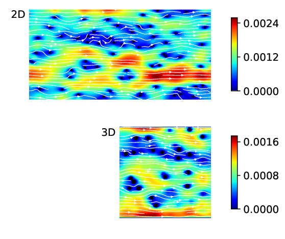
This paper is organized as follows. In Sec. 2 we review the expansion of a EDF in terms of orthogonal polynomials. We also discuss the special case of a weight function equal to the EDF itself. In Sec. 3 we show the generalized polynomials. In Sec. 4 the EDF is expanded up to fourth order in the set of new generalized polynomials orthonormal under a general weight. In Sec. 5 the EDF is expanded in polynomials orthonormal for the special case that the weight is equal to the EDF itself, $\omega(\xi)=f^{eq}(\xi)$. In Subsec. 5.1 we directly derive the EDF to order N=2 without using the orthonormal polynomials just to confirm the rightness of our ideas. In Sec. 6, we derive the macroscopic equations for semiclassical fluids (i.e., mass, momentum and energy conservation equations) in the context of the generalized polynomials. A discussion is made about the minimum order that the EDF should be expanded in order to recover each macroscopic equation. In Sec. 7, we calculate the forcing term for a second order expansion of the semiclassical EDF and verify that it satisfies the moment constraints up to second order. In Sec. 8, we obtain the quadratures and calculate the discrete weights of the $D1V3$, $D2V9$, and $D3V15$ lattices (more quadratures can be found in A). They are calculated for a generic weight function similarly to the polynomials. In Sec. 9, we develop our LBM for electrons in metals in two (2D) and three (3D) dimensions and perform three numerical tests: the Riemann problem, the Poiseuille flow and the Ohm’s law. In Sec. 10, we summarize our main results and conclude.

The equilibrium distribution function (EDF) $f^{(eq)}(\boldsymbol{\xi})$ is a central quantity in the Boltzmann-BGK framework since the non-equilibrium distribution function $f$ relaxes to the EDF, $f^{eq}$, within time $\tau$, according to,

where $\boldsymbol{\xi}$ and $\boldsymbol{a}$ are the microscopic velocity and acceleration, the latter defined by the external applied force. From this equation one obtains the hydrodynamical quantities under the Chapman-Enskog assumption, which says that expectation values over the microscopic velocity, $\boldsymbol{\xi}$, can be computed either from the non-equilibrium distribution function, $f(\boldsymbol{\xi})$, or from the equilibrium one, $f^{(eq)}(\boldsymbol{\xi})$. In this case the first three macroscopic moments are given by,

They correspond to the mass density $\rho$, the macroscopic velocity $\boldsymbol{u}$, and the temperature related quantity $\bar{\theta}$, which gives a measure of the energy density $\varepsilon=D\bar{\theta}/2$ (for the classical case, it is the temperature itself: $\bar{\theta}=\theta$). Therefore the use of $f(\boldsymbol{\xi}-\boldsymbol{u})$ instead of $f^{(eq)}(\boldsymbol{\xi}-\boldsymbol{u})$ renders the same values at any position and time for $\rho$, $\boldsymbol{u}$, and $\bar{\theta}$ according to the Chapman-Enskog assumption. We also define for later purposes the quantity $g$ associate to the fourth order expectation value,

which is a function of the same parameters that define $\rho$ and $\bar{\theta}$. Notice that the definition of the macroscopic velocity $\boldsymbol{u}$ is just the statement that at the local center of mass there is no net motion.

The D-dimensional Euclidean space is endowed with the following tensors, defined by Harold Grad [30], that can be expressed as sums of products of the Kronecker’s delta function ($\delta_{ij}=1$ for $i=j$ and 0 for $i\neq j$),

Properties of the above tensors, such as their number of terms, is discussed in more details Ref. [31].

Using the Chapman-Enskog expansion [32, 1], the macroscopic equations and the transport coefficients for a fluid governed by a given EDF $f^{eq}$ can be calculated from the discrete Boltzmann equation,

where $\Delta t$ is the step time. The continuous form of this equation is obtained by expanding in powers of $\Delta t$ and the first order term is the continuous Boltzmann equation, given Eq.(1).

We are interested in expanding the EDF in a polynomial power series in D-dimensional space, as such,

$\mathcal{A}_{i_{1}\,i_{2}\cdots i_{N}}$ are the projections of the EDF on the polynomials and $\mathcal{P}_{i_{1}\cdots i_{N}}(\boldsymbol{\xi})$ are the polynomials themselves, which are orthonormal under a generic weight function $\omega(\boldsymbol{\xi})$. This weight function is assumed to only depend on the modulus of the microscopic velocity $\boldsymbol{\xi}\equiv(\xi_{1},\xi_{2},\cdots,\xi_{D})$: $\omega(\boldsymbol{\xi})=\omega(\xi)$, $\xi\equiv|\boldsymbol{\xi}|$, and to have the property that $\omega(\boldsymbol{\xi})\rightarrow 0$ for $\xi\rightarrow\infty$ faster than any power of $\xi$.

Remarkably only a few terms in the above series expansion must be included to guarantee mass, momentum and energy conservation. The Chapman-Enskog analysis shows that in order to obtain the hydrodynamic equations of continuity and the Navier-Stokes equation the above series expansion can be cutoff at K=3 and to include the equation of energy conservation one must include only one more term, namely, go to order K=4. More details about the obtainment of the macroscopic equations can be found in Sec. 6. However the above cutoff procedure does not guarantee convergence of the cutoff series expansion to the orginal EDF. Hence it remains another very important requirement to be fullfilled which is of convergence to the underlying physics. This is expected under the assumption that the macroscopic velocity is much smaller than the microscopic one, $u\ll\xi$. The point that we stress here is that clearly this convergence is intimately connected to the choice of the weight function $\omega(\xi)$, that must be close enough to $f^{(eq)}(\xi)$ such that the remaining multiplying series is just a small correction to it and so, only a few terms would be enough to describe the corrections in $\boldsymbol{\xi}$.

The three EDFs explicitly depend on the microscopic velocity, $\boldsymbol{\xi}$, and implicitly on the position, $\boldsymbol{x}$, through the local macroscopic parameters, such as the density $\rho(\boldsymbol{x})$, the chemical potential $\mu(\boldsymbol{x})$, the fugacity $z(\boldsymbol{x})$ the macroscopic velocity $\boldsymbol{u}(\boldsymbol{x})$, and the temperature $\theta(\boldsymbol{x})$. The FD ($+$) and the BE ($-$) EDFs are given by

and the MB is,

where $\rho_{0}$ is a dimensionless density. All variables are defined dimensionless $(m=k_{B}=c=\hbar=e=1)$ by means of appropriate temperature and velocity scales. We observe the remarkable property of the series expansion in terms of the new polynomials, which is to have the macroscopic velocity expressed always as a ratio to a reference velocity of the problem, not necessarily the thermal velocity. For instance, notice that, in case of electron’s in metals, Mach’s number diverges at $T=0$ and cannot even be considered as a reference velocity. Indeed in this case the scale is set by the Fermi speed, $v_{F}$ and, since the microscopic velocity $U$ is very low in metals, for typical electric fields, $u/v_{F}\sim 0.4\times 10^{-6}$, according to previously given values. Hence the new polynomials in case of electrons in metals render the series expansion of the EDF at $T=0$ to be automatically in powers of the ratio $u/v_{F}$ instead, as shown in Ref. [9].

The convergence problem is better understood in the limit of a vanishing macroscopic velocity at Eq.(9), which gives that,

$f^{(eq)}(\boldsymbol{\xi})$ for the MB EDF is a gaussian and so the choice of $\omega(\xi)$ equal to the Hermite weight function,

is a good choice which implies the presence of the D-dimensional Hermite polynomials. However the Hermite weight is very different from the FD or MB EDFs rendering the need of many terms in the series expansion that multiplies $\omega(\xi)$. A striking example of such difficulty is provided by the FD EDF very near to zero temperature ($\theta\approx 0$) which becomes equal to a Heaviside step function ($f^{(eq)}_{\,FD}\approx 1$ for $\boldsymbol{\xi}^{2}/2\leq\mu$ and $f^{(eq)}_{\,FD}\approx 0$ for $\boldsymbol{\xi}^{2}/2\geq\mu$). Expressing the Heaviside function as the product of a gaussian times a series expansion implies that the latter must contain many terms. Hence this zero limit provides evidence of the inadequacy of the Hermite weight to describe electrons in metals for instance, since those behave at room temperature very similarly to the zero temperature limit [6]. Hence we reach the conclusion that for indistinguishable particles, namely BE or FD particles, the weight function must be chosen accordingly in order to reach convergence in the expanded EDF with a few terms. In this paper we study separately two similar but distinguishable situations, namely, of the weight similar to the EDF itself, $\omega(\xi)\approx f^{(eq)}(\boldsymbol{\xi})$ and of the weight exactly equal to the EDF, $\omega(\xi)=f^{(eq)}(\boldsymbol{\xi})$. In order to treat these two cases we firstly obtain the D-dimensional polynomials orthonormal under a general weight $\omega(\xi)$.

The orthonormality condition satisfied by the polynomials in this D-dimensional Euclidean space is given by,

The polynomials $\mathcal{P}_{i_{1}\cdots i_{N}}(\boldsymbol{\xi})$ are expressed in terms the components $\xi_{i}$ and of the Kronecker´s delta function, $\delta_{ij}$. The N${}^{\mbox{th}}$ order polynomial is symmetrical in the indices $i_{1}\cdots i_{N}$, and its parity is $(-1)^{N}$.

The N^th order polynomial is the sum of all possible symmetric tensors built from products of $\xi_{i}$ and of $\delta_{ij}$ times coefficients which are themselves polynomials in $\xi^{2}$ to maximum allowed power. This recipe yields a unique expression for the N^th order polynomial. As a working example we take the first five (N=0 to 4) polynomials,

These first five polynomials sum to a total of 14 coefficients (1 for N=0, 1 for N=1, 3 for N=2, 3 for N=3 and 6 for N=4) to be determined from the orthonormality condition of Eq.(14). The explicit orthonormalization procedure of the first five polynomials (N=0 to 4) produces exactly the 14 equations needed to determine them ($c_{K}$ for $K=0,1,2,3,4$, ${c^{\prime}}_{K}$ for $K=2,3,4$, ${\bar{c}}_{K}$ for $K=2,3,4$, $d_{4}$, ${d^{\prime}}_{4}$ and ${\bar{d}}_{4}$). This remarkable matching between the orthonormality condition and the D-dimensional Euclidean space symmetry group makes us conjecture that the present method of determining the coefficients can be extended to the N^th order. There is a deep tensorial structure behind the orthonormal condition of Eq.(14). This structure and the number of terms in tensors defined in Eqs.(6) and (7) are discussed elsewhere in Ref. [31].

The coefficients of the polynomials are solely functions of the weight $\omega(\xi)$ through the integrals $I_{N}$, which are central to the present study. They are assumed to exist and to have well defined properties.

By symmetry it holds that $I_{2N+1}=0$ since the integral vanishes. Using the spherical integration volume, $\int d^{D}\boldsymbol{\xi}\,\omega(\boldsymbol{\xi})=D\pi^{D/2}/\Gamma(D/2+1)\int d\xi\,\xi^{D-1}\omega(\xi)$, the $I_{2N}$ integrals become,

The explicitly derivation of the coefficients by imposing the orthonormality of the first five polynomials is carried in Ref. [31]. The coefficients can be summarized as follows:

where $\delta_{L}\equiv 2I_{L+2}I_{L-2}/\Delta_{L}^{2}$.

The well-known D-dimensional Hermite polynomials are just a particular case of the present polynomials for the case of a Hermite weight,

To obtain the integrals $I_{2N}$ of Eq.(16), we note that for the above $\omega(\xi)$,

Then it follows from Eq.(18) that,

In this limit $c_{K}=1$, $\bar{c}_{K}=0$ $c^{\prime}_{K}=-1$, $d_{4}=1$, $\bar{d}_{4}=0$ and $d^{\prime}_{4}=0$, and the polynomials become,

The tensorial basis that spans the new generalized polynomials contains the basis that spans the Hermite polynomials but not vice-versa. The D-dimensional Hermite polynomials $\mathcal{P}_{i_{1}\cdots i_{N}}$ are symmetric tensors in the indices $i_{1}\cdots i_{N}$ spanned over the basis formed by the tensors,

This basis is not large enough to span the new generalized polynomials, $\mathcal{P}_{i_{1}\cdots i_{N}}$, which demand a larger basis formed by the tensors

whose scalar functions $F\big(\xi\big)$ are polynomials in powers of the vector modulus, $1$, $\xi^{2}$, $\xi^{4}$, …,$\xi^{2k}$.

In this section, we consider the series expansion in polynomials orthonormal under a general weight $\omega(\xi)$. Although we are ultimately interested in the situation that the weight is similar to the EDF itself, $\omega(\xi)\approx f^{(eq)}(\boldsymbol{\xi})$, because this makes convergence faster, we do no take this assumption here. For the special case that $\omega(\xi)=f^{eq}(\xi)$ some extra properties can be derived and this is done in the next section. The projections $\mathcal{A}_{i_{1}\,i_{2}\cdots i_{N}}$ are obtained from the general orthonormal relation of Eq.(14),

There is a completeness relation for these generalized tensorial polynomials, which is obtained from the above expression and Eq.(9):

since $f(\boldsymbol{\xi}-\boldsymbol{u})=\int d^{D}\boldsymbol{\xi^{\prime}}\,\delta^{D}(\boldsymbol{\xi^{\prime}}-\boldsymbol{\xi})f(\boldsymbol{\xi^{\prime}}-\boldsymbol{u})$. The completeness relation is given by,

In terms of the relative (or peculiar) velocity $\boldsymbol{\eta}=\boldsymbol{\xi}-\boldsymbol{u}$ the quantities $\rho$, $\bar{\theta}$ and $g$ become,

For the case of the FD-BE EDF these quantities can be expressed in terms of the integrals defined as

which are functions of the fugacity $z$. One obtains that,

Recall that the EDF is solely a function of the modulus of the relative velocity, namely, $f^{eq}(\eta)$, $\eta=|\boldsymbol{\eta}|$. Below the first five projections of the EDF are calculated by noticing that by taking that $d^{D}\boldsymbol{\xi}=d^{D}\boldsymbol{\eta}$ the limits of integration do not change since the integrand vanishes exponentially at infinity.
$\bullet$ Zeroth order – Since $\mathcal{P}_{0}(\boldsymbol{\xi})=c_{0}$, one obtains that