Steady states and edge state transport in topological Floquet-Bloch systems

Periodic driving has recently attracted interest as a promising tool for exploring new phases of quantum matter  [1, 2, 3, 4, 5, 6, 7, 8, 9, 10, 11, 12, 13, 14, 15, 16, 17, 18, 19]. Beyond accessing phases resembling those accessible in equilibrium, “Floquet systems” also support anomalous, intrinsically non-equilibrium dynamical phases [20, 21, 15, 16, 17, 18, 19, 22, 23, 24, 25]. Topological properties and spectra of periodically driven systems have been demonstrated in experiments in solid state [26, 27], cold atoms [28, 29, 30, 31, 32], and optical systems [33, 34].

In this work we focus on Floquet topological insulators (FTIs): systems in which a topological Floquet band structure is induced in a topologically-trivial system by a time-periodic drive [6]. Investigating the complex non-equilibrium steady-states that result from the unavoidable coupling to bath degrees of freedom, such as phonons, is essential for understanding the physical properties of Floquet systems [35, 36, 37, 38, 39, 40]. In particular, when the system is longer than the inelastic mean free path (MFP), transport depends crucially on the interplay between the coupling to the system’s leads and to its intrinsic baths. We thus seek to characterize these steady states, and to understand their physical manifestations.

In the present study we consider two-dimensional (2D) systems in which a resonant drive is used to induce a band inversion in the Floquet-Bloch spectrum (see Fig. 1). The resulting Floquet bands have non-zero Chern numbers, and in a finite geometry with edges exhibit chiral Floquet edge modes. In this work we will be particularly interested in the steady states of the chiral Floquet edge modes, and their coexistence with the non-equilibrium steady state of the bulk.

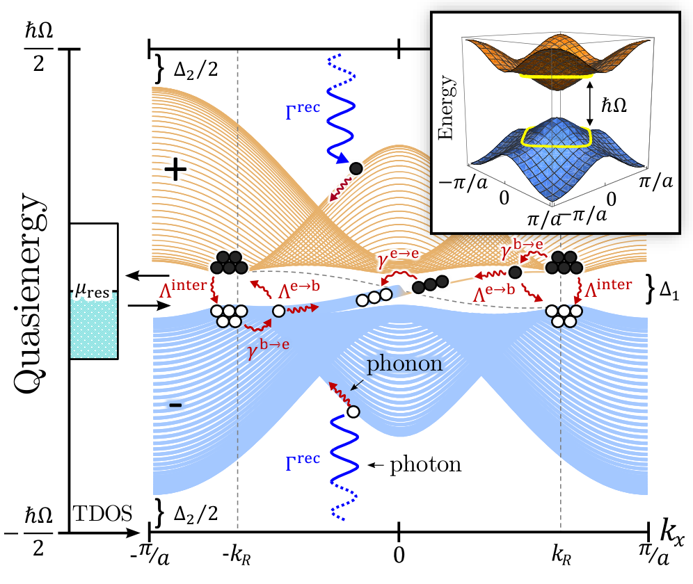
In a driven electronic system, the natural intrinsic baths to consider are the phonons of the crystal lattice and the photons of the ambient electromagnetic environment. In the system we consider, the role of acoustic phonons is mainly to relax momentum and (quasi)energy, while photon emission associated with particle-hole recombination acts as a primary heating source in the Floquet band picture (similar considerations were applied to one-dimensional systems in [39]). Due to the edges of the system, the steady state is inhomogeneous, and therefore we analyze the system using a full Floquet-Boltzmann approach [41]. To deduce the transport properties of the system, we also consider the effects of a coupling to an external Fermi reservoir (i.e., a lead).

Below we show that the steady-state, characterized by the populations of Floquet-Bloch states, resembles that of a topological insulator, with an additional non-equilibrium Fermi sea of electrons and holes in the bulk. The chiral Floquet edge states are populated according to a smooth distribution with a well defined Fermi level. In the presence of coupling to an energy-filtered Fermi reservoir, whose chemical potential lies in the Floquet band gap [39], we find that: (1) the bulk excitation density is insensitive to variations of the reservoir chemical potential; (2) the Fermi level of the edge states is pinned to the chemical potential of the reservoir. Using these results, we assess the stability of the edge currents and give prospects for measuring edge transport in Floquet topological insulators.

We now introduce the model for the driven system. We consider a two-band 2D model, described in the absence of driving by the Hamiltonian

where $\boldsymbol{{\sigma}}=\left({\sigma}^{x},{\sigma}^{y},{\sigma}^{z}\right)$ is the vector of Pauli matrices, and $\hat{c}_{\boldsymbol{k}{\nu}}^{\dagger}$ creates an electron with quasimomentum $\boldsymbol{k}$ and pseudospin ${\nu}=\left\{\uparrow,\downarrow\right\}$. We take $\textbf{d}(\boldsymbol{k})=(A\sin(ak_{x}),A\sin(ak_{y}),M-4B+2B\cos(ak_{x})+2B\cos(ak_{y}))$, such that Eq. (1) describes half the degrees of freedom in the BHZ model for time-reversal invariant semiconductor quantum wells [42, 43, 44]. Here $A,B$ and $M$ are material-dependent parameters, and $a$ is the lattice constant of the crystal. We assume a trivial semiconductor (with non-inverted band structure), with $M>0$ and $B<0$.

The semiconductor is periodically driven by an external field with an above-gap frequency ${\Omega}$. For simplicity we consider a uniform driving field of amplitude $V_{0}$ that couples to electrons through ${\sigma}^{z}$ ¹⁰¹⁰ 10 More realistic time-dependent electromagnetic fields can be incorporated in this model, see [6], modeled by the time-dependent Hamiltonian

Below we work in the basis of Floquet-Bloch eigenstates of the time-periodic single particle Hamiltonian $\hat{\mathcal{H}}_{0}+\hat{\mathcal{H}}_{V}(t)=\sum_{\boldsymbol{k}}\hat{c}_{\boldsymbol{k}{\nu}}^{\dagger}\left[H(t)\right]_{\boldsymbol{k},{\nu}{\nu}^{\prime}}\hat{c}_{\boldsymbol{k}{\nu}^{\prime}}$. The Floquet eigenstates satisfy $\left(i\hbar\frac{\partial}{\partial t}-H(t)\right)|{{\psi}(t)}\rangle=0$, with $|{{\psi}(t)}\rangle=e^{-i{\varepsilon}t/\hbar}|{\phi(t)}\rangle$. Here $|{{\phi}(t)}\rangle=|{{\phi}(t+T)}\rangle$ is periodic with period $T=2\pi/\Omega$, and ${\varepsilon}$ is the quasienergy. Throughout, we use the convention $-\hbar\Omega/2\leq{\varepsilon}<\hbar\Omega/2$.

The driving field yields resonant transitions between the valence and conduction bands along a closed curve in momentum space, see Fig. 1 (inset). A gap of magnitude $\Delta_{1}\propto|V_{0}|$ opens at quasienergy ${\varepsilon}=0$, yielding two separate quasienergy bands. The driving field leads to an effective band inversion of the Floquet bands with respect to the original non-driven band structure. An important consequence of this band inversion is the appearance of chiral edge states in the gap at ${\varepsilon}=0$ for a system in a finite geometry with edges [6]. We restrict $\hbar\Omega>|M-8B|$, such that there is only a single-photon resonance.

We label the bulk Floquet states by the quasimomentum $\boldsymbol{k}$ and a Floquet band index ${\alpha}=\pm$ (distinct from the band index of the non-driven system): $|{{\psi}_{\boldsymbol{k}{\alpha}}(t)}\rangle=e^{-i{\varepsilon}_{{\alpha}}(\boldsymbol{k})t/\hbar}\sum_{m}e^{im{\Omega}t}|{{\phi}^{m}_{\boldsymbol{k}{\alpha}}}\rangle$ [46, 47]. We refer to the Floquet bands with quasienergies $0<{\varepsilon}<\hbar{\Omega}/2$ and $-\hbar{\Omega}/2<{\varepsilon}<0$ as the upper $(+)$ and lower $(-)$ Floquet bands, respectively, see Fig. 1.

In the following, we will consider a system with periodic boundary conditions in the $x$ direction, and open boundary conditions in the $y$ direction. As seen in Fig. 1, in this geometry the edge states exist for quasimomentum $k_{x}$ in the interval $-k_{R}\lesssim k_{x}\lesssim k_{R}$, where $k_{R}$ is the maximal value of $k_{x}$ for which the driving field is resonant. We denote the Floquet edges states as $|{\chi_{k_{x}{\beta}}(t)}\rangle$, where the label ${\beta}$ corresponds to the left (L) and right (R) edges (at $y=0$ and $y=L_{y}$), for which $\partial{\varepsilon}/\partial k_{x}$ is negative and positive, respectively, see Fig. 2a.

The open, driven system evolves to a steady state, governed by its coupling to one or more heat baths (taken to be at zero temperature). We first focus on the bosonic bath, and consider the roles of acoustic phonons and photons (associated with radiative recombination). Using the label ${\lambda}=\ell,s$ to denote the photon (light) and acoustic phonon (sound) modes, we describe the dynamics of each mode by the Hamiltonian

Here $\hat{b}_{{\lambda},\boldsymbol{q}}^{\dagger}$ are creation operators of ${\lambda}$-bosons. The velocity $v_{\lambda}$ is taken to be constant and isotropic for each mode. While the electronic degrees of freedom are confined to a 2D plane, we take the bosonic bath modes to live in three dimensions; for simplicity we consider a single polarization mode for each boson type. For the (finite bandwidth) acoustic phonon bath, we take a linear dispersion up to a Debye frequency, $\omega_{D}$ ⁴⁰⁴⁰ 40 In this work we use simple models for the acoustic phonons and the electromagnetic environment, and their couplings to the system. More detailed modeling of these baths would not qualitatively change our results..

Inspired by the physics of semiconductor quantum wells, we assume that emission of a photon is accompanied by a pseudo-spin flip (corresponding to a change of one unit of electronic angular momentum). Furthermore, we take the interaction with acoustic phonons to conserve the pseudospin index, as acoustic phonons have suppressed matrix elements between different atomic orbitals. The Hamiltonian describing local interactions between electrons and ${\lambda}$-bosons thus reads:

where ${\eta}_{s}=g_{s}\mathds{1}$ for electron-phonon coupling, and ${\eta}_{\ell}=g_{\ell}{\sigma}^{+}$ for electron-photon coupling. The quantities $g_{\ell}$ and $g_{s}$ denote the associated coupling strengths. In Eq. (4), the coordinate $\boldsymbol{r}$ is confined to the 2D plane.

In closing this section defining the model, we note that the full Hamiltonian possesses particle-hole and inversion symmetry at all $t$. The system’s Floquet spectrum and the kinetic equations derived below exhibit corresponding symmetries. However, our qualitative conclusions do not depend on these symmetries.

Before diving into the full kinetic equation, we first characterize the steady states using a simplified phenomenological model, which takes into account the most significant contributions to the population kinetics in the system (see Fig. 1). In the following discussion, we restrict our attention to a half-filled system.

Generically, the population kinetics in a driven system differs from that of a system in thermal equilibrium, due to scattering processes in which the total quasienergies of the incoming and outgoing modes differ by integer multiples of $\hbar\Omega$. As a starting point, we first consider a system in which the sums of quasienergies of the incoming modes and outgoing modes are strictly equal in all scattering processes (which requires the system-bath coupling to obey special conditions [49, 50, 51, 52, 53]). In this situation, the steady state of the driven system is simply given by a Fermi-Dirac distribution in terms of the Floquet bands, with the ordering of quasienergies (i.e., choice of Floquet-Brillouin zone) as used in Fig. 1. The temperature of the distribution is that of the phonon bath. For a half-filled system, we obtain an ideal FTI: when the bath is at zero temperature, the lower (upper) Floquet band is filled (empty), and the edge state is filled up to the Fermi level at $\varepsilon=0$ (corresponding to $k_{x}=0$).

Our goal is to obtain the steady state of the system in the presence of all scattering processes, including those where the total quasienergy changes by a multiple of $\hbar\Omega$. These “Floquet-Umklapp” processes create excitations from the lower to the upper Floquet band, and thereby act as a source of “heating” in the Floquet basis. We characterize the steady state in the bulk by the density of excited electrons in the “upper” (+) bulk Floquet band, $n_{\rm b}=\int\frac{d^{2}\boldsymbol{k}}{(2{\pi})^{2}}\langle\hat{\psi}^{\dagger}_{\boldsymbol{k}+}(t)\hat{\psi}_{\boldsymbol{k}+}(t)\rangle$. At each edge the steady state is characterized by the density of excited particles above the Fermi level of the ideal FTI (${\varepsilon}=0$). For the right edge, this density is given by $n_{\rm e}=\int_{0}^{k_{R}}\frac{dk_{x}}{2{\pi}}\langle\hat{\chi}^{\dagger}_{k_{x}R}(t)\hat{\chi}_{k_{x}R}(t)\rangle$. The operators $\hat{\psi}^{\dagger}_{\boldsymbol{k}{\alpha}}(t)$ and $\hat{\chi}^{\dagger}_{k_{x}{\beta}}(t)$ create electrons in the bulk and edge Floquet states $|{{\psi}_{\boldsymbol{k}{\alpha}}(t)}\rangle$ and $|{\chi_{k_{x}{\beta}}(t)}\rangle$, respectively ⁵⁰⁵⁰ 50 The operators $\hat{\psi}^{\dagger}_{\boldsymbol{k}{\alpha}}(t)$ and $\hat{\chi}^{\dagger}_{k_{x}{\beta}}(t)$ obey the anticommutation relations $\{\hat{\psi}^{\dagger}_{\boldsymbol{k}{\alpha}}(t),\hat{\psi}_{\boldsymbol{k}^{\prime}{\alpha}^{\prime}}(t)\}=\delta_{\boldsymbol{k}\boldsymbol{k}^{\prime}}\delta_{{\alpha}{\alpha}^{\prime}}$ and $\{\hat{\chi}^{\dagger}_{k_{x}{\beta}}(t),\hat{\chi}_{k_{x}^{\prime}{\beta}^{\prime}}(t)\}=\delta_{k_{x}k_{x}^{\prime}}\delta_{\beta\beta^{\prime}}$.. The distributions of electrons in states with $\varepsilon>0$ and of holes in states with $\varepsilon<0$ are related by particle hole symmetry (see below). Additionally, the distributions in the right and left edge states are related by inversion symmetry.

For a semiconductor with a sufficiently large band gap, such that $M\gg\hbar\omega_{\rm D}$, Floquet-Umklapp processes resulting from phonon scattering are suppressed as $[V_{0}/(\hbar\Omega)]^{4}$ [39]. For simplicity, in our analysis we will assume that all Floquet-Umklapp process are due to radiative recombination. Since this process involves emission of a photon, it predominately contributes when the characters of the initial and final states correspond to the conduction and valence bands of the undriven system, respectively (recall that the electron-photon coupling is off-diagonal in pseudospin). Close to the ideal FTI steady state, $\boldsymbol{k}$-modes in the lower Floquet band with momenta inside the resonance curve are filled, and have a conduction band character, while those of the upper band are empty and have valence band character. Radiative recombination between these states leads to a source term for particles in the upper Floquet band, $\dot{n}_{\rm b}=\Gamma^{\rm rec}$ (see Fig. 1), with rate $\Gamma^{\rm rec}$ approximately independent of the excitation density for small deviations from the ideal FTI state.

Once excited to the upper Floquet band, electrons quickly relax to the band minima due to scattering by phonons. Near the Floquet band minima (around the resonance curve), the Floquet states are hybridized superpositions of valence and conduction band states. This hybridization allows phonons to scatter electrons from these minima to empty states near the maxima of the lower Floquet band. Consider the rate of such phonon-assisted “recombination” of Floquet-band carriers. During such a process, an electron in the upper band must find a hole in the lower band. The resulting rate is thus proportional to the density of electrons times that of the holes (which are equal at half filling): $\dot{n}_{\text{b}}\approx-\Lambda^{\rm inter}n_{\text{b}}^{2}$.

Next, we account for processes which scatter particles between bulk and edge states. Such bulk-edge scattering processes are predominantly phonon-assisted (the rates for photon-assisted bulk-edge scattering are suppressed by a small density of states). Assuming a small population of excited electrons (with ${\varepsilon}>0$) on the edge, $n_{\rm e}\ll 1/a$, bulk-to-edge processes predominantly take excited electrons in the upper Floquet band to the nearly empty $k$-space region of the edge states (with $k_{x}>0$, for the right edge). In contrast, edge-to-bulk processes require that the scattered edge electron finds an empty bulk state (i.e., a hole) in the lower Floquet band (see Fig. 1). The corresponding rate is thus proportional to both the densities of excitations on the edge and in the bulk. We therefore estimate the contribution of bulk-edge processes to $\dot{n}_{\rm e}$ as $\dot{n}_{\rm e}={\gamma}^{\rm b\to e}n_{\rm b}-{\Lambda}^{\rm e\to b}n_{\rm b}n_{\rm e}$. The parameters ${\gamma}^{\rm b\to e}$ and $\Lambda^{\rm e\to b}$ encode the rates of bulk-to-edge and edge-to-bulk scattering processes, respectively.

Last, we account for phonon-assisted scattering of particles within the edge. At low phonon temperatures, such processes predominately decrease the quasienergy of the electrons, and thus tend to decrease the density of excited particles on the edge. The requirement that an excited edge-electron finds an edge-hole gives $\dot{n}_{\rm e}=\gamma^{\rm e\to e}n_{\rm e}^{2}$.

Summing up the processes above, we arrive at the rate equations for the bulk and edge excitation densities:

The steady state solution for the above equations is obtained for $\dot{n}_{\rm b}=\dot{n}_{\rm e}=0$.

In the thermodynamic limit, the rate parameters in Eq. (5) become independent of system size [55]. Note that in Eq. (5a), the source term for the 2D density $n_{\rm b}$ due to coupling to the 1D edge is multiplied by a factor of $1/L_{y}$. Thus for $L_{y}\to\infty$, Eq. (5a) yields a bulk excitation density $n_{\rm b}$ which is independent of $n_{\rm e}$, and scales as

As expected, the bulk excitation density is unaffected by the presence of the edge. The dimensionless parameter ${\kappa}a^{4}$ captures the competition between “heating” (Floquet-Umklapp) and “cooling” processes in the bulk.

The rates controlling the excitation density on the edge in Eq. (5b) are predominantly due to phonon-assisted scattering. Therefore their ratios do not scale with $\kappa$. For sufficiently small $\kappa$, we reach $\frac{{\gamma}^{\rm e\to e}{\gamma}^{\rm b\to e}}{({\Lambda}^{\rm e\to b})^{2}}\gg n_{\text{b}}$. In this limit, the second term in Eq. (5b) can be omitted and we find for the steady state:

where the ratio ${\gamma}^{\rm b\to e}/{\gamma}^{\rm e\to e}$ is independent of ${\kappa}$.

The bulk excitation density $n_{\text{b}}$ estimated in Eq. (8) represents a spatial average over the full system. In a more detailed picture, we expect the excitation density to be inhomogeneous, deviating from the bulk value estimated in Eq. (8) near the edges. We investigate the spatial dependence of $n_{\rm b}$ below.

We now turn to a more microscopic treatment, and characterize the steady state using a Floquet-Boltzmann equation approach. We focus on the regime where the MFP is larger than the characteristic wavelength of electrons. We characterize the steady state in the bulk in terms of a phase space distribution function $f^{\text{b}}_{\boldsymbol{k}{\alpha}}(\boldsymbol{r};t)$. Due to the translational invariance of the cylinder, we assume that the phase space distribution is independent of $x$. Therefore we define:

Note that $\int\!\!\frac{d^{2}\boldsymbol{k}}{(2\pi)^{2}}f^{\text{b}}_{\boldsymbol{k}{\alpha}}(y;t)$ gives the density of electrons in band $\alpha$ at position $y$ (for any $x$), at time $t$. A dependence on $y$ is expected due to the edges at $y=0,L_{y}$ ¹²¹² 12 Off-diagonal correlations between states separated with large gaps, on the scale of the scattering rates vanish [78, 39].. The distributions within the one-dimensional edge states are defined as $f^{\text{e}}_{k_{x}{\beta}}(t)=\langle\hat{\chi}_{k_{x}{\beta}}^{\dagger}(t)\hat{\chi}_{k_{x}{\beta}}(t)\rangle$.

Next, we study the steady-state behaviour of $f^{\text{b}}_{\boldsymbol{k}{\alpha}}(y)$. The physics on length scales larger than the MFP is described by the Floquet-Boltzmann equation [41],

Here $v_{y,{\alpha}}(\boldsymbol{k})=\hbar^{-1}\partial_{k_{y}}{\varepsilon}_{\alpha}(\boldsymbol{k})$ is the Floquet band group velocity in the $y$ direction, and the collision integrals $\mathcal{I}^{\text{b}\text{b}}_{\boldsymbol{k}{\alpha}}$, $\mathcal{I}^{\text{b}\text{R}}_{\boldsymbol{k}{\alpha}}$, and $\mathcal{I}^{\text{b}\text{L}}_{\boldsymbol{k}{\alpha}}$ describe bulk-bulk, bulk-right-edge and bulk-left-edge scattering processes, respectively. For brevity, in Eq. (9) we used $f^{\text{b}}_{\boldsymbol{k}{\alpha}}\equiv f^{\text{b}}_{\boldsymbol{k}{\alpha}}(y;t)$; likewise, we suppressed the dependence of the collision integrals on $y$ and $t$. The Boltzmann equation for the edges has a similar structure, namely, $\partial_{t}f^{\text{e}}_{k_{x}{\beta}}=\mathcal{I}^{\text{e}\text{e}}_{k_{x}{\beta}}+\mathcal{I}_{k_{x}{\beta}}^{\text{e}\text{b}}$.

In explicit form, the collision integral for bulk-to-bulk scattering processes is given by

where $W_{\boldsymbol{k}^{\prime}{\alpha}^{\prime}}^{\boldsymbol{k}{\alpha}}$ is the total scattering rate from $(\boldsymbol{k},{\alpha})$ to $(\boldsymbol{k}^{\prime},{\alpha}^{\prime})$. The rates $W_{\boldsymbol{k}^{\prime}{\alpha}^{\prime}}^{\boldsymbol{k}{\alpha}}$ in Eq. (10) are $y$-independent, and therefore any $y$ dependence of $\mathcal{I}^{\text{b}\text{b}}_{\boldsymbol{k}{\alpha}}$ arises through the distributions $f^{\text{b}}_{\boldsymbol{k}{\alpha}}(y;t)$. In contrast, for the bulk-edge collision integrals $\mathcal{I}_{\boldsymbol{k}{\alpha}}^{\text{b}\text{R}}$ and $\mathcal{I}_{\boldsymbol{k}{\alpha}}^{\text{b}\text{L}}$ the corresponding rates themselves are only significant for values of $y$ near the edges, due to the spatial profile of the edge states. The full expressions for all the collision integrals can be found in the Supplementary Material [55].

The rate $W_{\boldsymbol{k}{\alpha}}^{\boldsymbol{k}^{\prime}{\alpha}^{\prime}}$ in Eq. (10) can be written as a sum of phonon ($s$) and photon ($\ell$) assisted scattering rates, $W_{\boldsymbol{k}{\alpha}}^{\boldsymbol{k}^{\prime}{\alpha}^{\prime}}=W_{\ell,\boldsymbol{k}{\alpha}}^{\boldsymbol{k}^{\prime}{\alpha}^{\prime}}+W_{s,\boldsymbol{k}{\alpha}}^{\boldsymbol{k}^{\prime}{\alpha}^{\prime}}$, given by

The DOS of ${\lambda}$-bosons is given by ${\rho}_{{\lambda}}({\varepsilon},\boldsymbol{q})=\frac{a^{2}}{L_{x}L_{y}}\frac{a{\varepsilon}{\Theta}({\varepsilon}-\hbar v_{\lambda}\left|\boldsymbol{q}\right|)}{{\pi}\hbar v_{\lambda}\sqrt{{\varepsilon}^{2}-\hbar^{2}v_{\lambda}^{2}\left|\boldsymbol{q}\right|^{2}}}$, where (as above) $\lambda=\{s,\ell\}$. For relatively low energy emission processes [e.g., relaxation across the Floquet gap, contributing to $\Lambda^{\rm inter}$ in Eq. (5b)], the photon DOS is suppressed relative to the phonon DOS by $v_{s}/v_{\ell}$ and phonon-emission dominates. For high energy transfers, the DOS of phonons vanishes when ${\varepsilon}$ is above the Debye energy, $\hbar{\omega}_{D}$. In this work we fix $\omega_{D}$ within the range ${\Delta}_{1}<\hbar{\omega}_{D}<{\Delta}_{2}$, ensuring Floquet-Umklapp processes induced by phonon scattering are fully suppressed. Here $\Delta_{1}$ and $\Delta_{2}$ are the gaps centered at $\varepsilon=0$ and $\varepsilon=\hbar\Omega/2$, respectively, see Fig. 1.

Within this formalism, we can estimate the phenomenological rates in the effective model, Eq. (5), using microscopic parameters (for full details see [55]). We denote by $\mathcal{W}_{\boldsymbol{k}}^{\rm rec}=\left(\frac{L_{x}L_{y}}{4{\pi}}\frac{{\Omega}^{2}}{v_{\ell}^{2}}\right)W_{\ell,\boldsymbol{k}-}^{\boldsymbol{k}+}$ the recombination rate for particles initially in the lower Floquet band. This rate is significant within the resonance curve, where the Floquet bands are inverted and the characters of the initial and the final states correspond to the conduction and valence bands of the non-driven system, respectively. Thus the source term for the bulk excitation density is ${\Gamma}^{\rm rec}\approx\int\frac{d^{2}\boldsymbol{k}}{(2{\pi})^{2}}\mathcal{W}^{\rm rec}_{\boldsymbol{k}}\equiv\frac{A_{\mathcal{R}}}{(2{\pi})^{2}}\overline{\mathcal{W}}^{\rm rec}$, where $A_{\mathcal{R}}$ is the momentum-space area inside the resonance curve. We estimate the parameter $\Lambda^{\rm inter}$ characterizing phonon-assisted relaxation between Floquet bands as $\Lambda^{\rm inter}\approx L_{x}L_{y}\overline{\mathcal{W}}^{\rm inter}$, where $\overline{\mathcal{W}}^{\rm inter}=W_{s,\boldsymbol{k}_{R}+}^{\boldsymbol{k}_{R}-}$ is an average relaxation rate of a particle in the active region around the minimum of the upper Floquet band. With these definitions, we obtain an approximate expression for ${\kappa}$ in Eq. (6): ${\kappa}\approx\frac{A_{\mathcal{R}}{\Omega}^{2}v_{s}g_{\ell}^{2}}{8{\pi}^{3}v_{\ell}^{3}g_{s}^{2}}$. The parameters $\gamma^{\rm b\to e}$, $\Lambda^{\rm e\to b}$, and $\gamma^{\rm e\to e}$ can be estimated using the bulk-to-edge and edge-to-edge scattering rates in the same manner.

We now numerically solve Eq. (9) in the steady state, taking $\dot{f}_{\boldsymbol{k}{\alpha}}=0$. We consider the system at half-filling. Figure 3a shows the spatial dependence of the bulk excitation density, $n_{\text{b}}(y)=\int d^{2}\boldsymbol{k}f_{\boldsymbol{k}+}(y)$, for three values of $\kappa$. Away from the edges, the density reaches a position-independent “bulk” value, $n^{0}_{\text{b}}$. The dependence of $n^{0}_{\text{b}}$ on $\kappa a^{4}$ is shown in the inset of Fig 3a, and agrees well with our estimate in Eq. (6).

The spatial dependence of $n_{\rm b}(y)$ can be accounted for by generalizing Eq. (5a) to a reaction-diffusion equation  [39, 55]. From this picture we extract the “healing length” $\xi$ over which the excitation density relaxes to the bulk value $n^{0}_{\rm b}$: $\xi\approx\sqrt{Dn^{0}_{\rm b}/(2\Gamma_{\rm rec})}$, where $D$ is the diffusion constant. Taking $D\approx\bar{v}^{2}\tau$, where $\bar{v}$ is a typical velocity of the excited carriers in the steady state and $\tau$ is the scattering time (due to phonons), we find good agreement with the length scales exhibited in our numerical results [55].

Figure 3b shows steady state distributions of the bulk far away from the edges, for three different values of ${\kappa}a^{4}$. The steady state distribution of the upper band is well described by a Floquet-Fermi-Dirac distribution (a Fermi-Dirac distribution in terms of the quasienergy spectrum), with an effective temperature and chemical potential obtained as fitting parameters. The distribution of the lower band is related by particle-hole symmetry, $f_{\boldsymbol{k},-}^{\text{b}}=1-f_{-\boldsymbol{k},+}^{\text{b}}$. The chemical potential describing the distribution in the upper band does not lie in the middle of the gap. Therefore, to describe the distribution of the system, we must use two separate Fermi-Dirac distributions, with distinct chemical potentials, for the upper and lower Floquet bands (for full analysis of the fit to the Floquet-Fermi-Dirac distribution, see [55]). Analogous distributions were found for a 1D system in Ref. [39]. In the absence of photon-assisted recombination (i.e., when ${\kappa}a^{4}\to 0$), the steady state converges to a global zero-temperature Gibbs state over the Floquet spectrum [49, 50, 51].

The steady state distribution of the particles along the right edge is shown in Fig. 3c. The distribution of the left edge is related by inversion symmetry, $f_{k_{x}\text{L}}^{\text{e}}=f_{-k_{x}\text{R}}^{\text{e}}$. We observe that the excitations in the edge states predominantly accumulate near $k_{x}\sim 0$. The shape of the distribution is approximated to a good accuracy by a “quasi Fermi-Dirac distribution,” defined as $f_{\rm QFD}({\varepsilon})=(1-{\delta})f_{\rm FD}({\varepsilon},T_{\text{e}})+{\frac{1}{2}}{\delta}$. Here $f_{\text{FD}}({\varepsilon},T_{\text{e}})$ is the conventional Fermi function, which we scale by a contrast factor ($0<{\delta}<1$) to create $f_{\rm QFD}$. The form of the function $f_{\rm QFD}$ dictates that the effective temperature $T_{\text{e}}$ is approximately proportional to the excitation density on the edge, $n_{\text{e}}$. The ${\delta}$-parameter describes a small density of particles (holes), uniformly spread along the $k_{x}>0$ ($k_{x}<0$) part of the edge mode. The electron and hole “pockets” at the extrema of the bulk Floquet bands provide the source for this excess density. Thus, we expect ${\delta}$ to exhibit a similar scaling with $\kappa$ as the density of bulk electrons $n_{\text{b}}$. The dependence of $n_{\rm e}a$, and of the fitted parameters $T_{\text{e}}$ and ${\delta}$ on ${\kappa}a^{4}$ are shown in Fig. 3a (inset) and Fig 3c. The results of our simulations are in a good agreement with Eqs. (6) and (7) and the scaling arguments above.

Can the topological properties of FTIs be identified by transport measurements? To study this question, we couple the system to Fermi reservoirs at the two edges, $y=0$ and $y=L_{y}$, see Fig. 2a. The Hamiltonian describing the right reservoir and its coupling to the system reads

Here we have introduced a super-index $p$ labeling system operators, Fourier transformed with respect to $x$: $p=\{k_{x},y,\nu\}$. Furthermore, $\hat{d}_{l}^{\dagger}$ is the creation operator for an electron in mode $|{l}\rangle$ of the right reservoir. For simplicity, we choose a system-lead coupling that does not introduce a preferred direction in pseudo-spin space. This is accomplished by taking two degenerate sets of modes, labeled by $l=\{k_{x},\mathcal{E}_{l},\nu\}$, where $\mathcal{E}_{l}$ is the mode’s energy (which is independent of $\nu=\{\uparrow,\downarrow\}$). The left reservoir and its coupling to the system are described in an analogous manner. We first consider the left and right reservoirs to have a common chemical potential, ${\mu}_{\rm res}$.

In general, the values of the couplings $J_{lp}$ depend on the precise forms of the reservoir states $|{l}\rangle$, and the details of the lead-system coupling. We take the couplings to be uniform in the $\hat{\boldsymbol{x}}$ direction; for the right lead, we specify $J_{lp}=J\delta_{yL_{y}}\delta_{\nu(p)\nu(l)}\delta_{k_{x}(p)k_{x}(l)}$. For the left lead we replace $\delta_{yL_{y}}$ with $\delta_{y0}$. (We do not expect our results to change qualitatively for other generic forms of the reservoirs and the couplings.)

In the following we will consider the effect of the leads when ${\mu}_{\rm res}$ is placed within the Floquet gap. Note that a Floquet state of the system with quasienergy ${\varepsilon}$ is coupled to reservoir states in a wide range of energies $\mathcal{E}_{l}={\varepsilon}+n\hbar{\Omega}$ via the harmonics $|{{\chi}_{k_{x}{\beta}}^{n}}\rangle$ (or $|{{\phi}_{\boldsymbol{k}{\alpha}}^{n}}\rangle$). As a result, if the reservoir’s density of states has a wide bandwidth, electrons occupying lead states below the Fermi level can tunnel into the upper Floquet band of the system. These processes (and similar processes for holes) increase the number of excited particles (holes) in the upper (lower) Floquet band, leading to deviations from the ideal Floquet insulator state. To avoid this deleterious effect, we couple the Fermi reservoir through a narrow band of “filter” states [39], which effectively limits the density of states of the Fermi reservoir. In our simulation, we take the reservoirs to have a box-shaped DOS of width $w$, aligned symmetrically around the center of a single Floquet zone, see Fig. 1.

The introduction of the system-lead coupling, $\hat{\mathcal{H}}^{R(L)}_{\rm res}$, adds additional collision integrals to the Boltzmann equations for the bulk and edge distributions. The collision integral describing scattering between the right reservoir and the right edge state is given by

Here $\mathcal{J}_{k_{x}\text{R}}^{n}=\frac{2{\pi}}{\hbar}|J|^{2}\sum_{l,\nu}\left|\langle k_{x},L_{y},\nu|\chi_{k_{x};\text{R}}^{n}\rangle\right|^{2}{\delta}({\varepsilon}^{n}_{\text{R}}(k_{x})-\mathcal{E}_{l})$, where $|k_{x},L_{y},\nu\rangle$ is the state created by $c^{\dagger}_{k_{x},y=L_{y},\nu}$ and ${\varepsilon}_{\text{R}}^{n}(k_{x})={\varepsilon}_{\text{R}}(k_{x})+n\hbar{\Omega}$; ${\varepsilon}_{\text{R}}(k_{x})$ is the quasienergy of the right edge state, with quasimomentum $k_{x}$. The values of $\mathcal{E}_{l}$ are limited to the range within the filter window. An identical expression holds for the left edge state, with $\text{R}\to\text{L}$. In addition, Eq. (9) contains a collision integral $\mathcal{I}^{\text{b},{\rm res}}_{\boldsymbol{k}{\alpha}}$ describing scattering directly between the leads and the bulk states. The rates appearing in this collision integral are significant only for $y$ values sufficiently close to the leads [55].

The coupling strength between the reservoir and the edge states is characterized by $\overline{\mathcal{J}}_{{\beta}}=\frac{1}{2k_{R}}\int_{-k_{R}}^{k_{R}}dk_{x}\mathcal{J}_{k_{x};{\beta}}^{0}$. When $\overline{\mathcal{J}}_{{\beta}}\gg{\Lambda}^{\rm e\to b}n_{\text{b}}$ (such that tunneling between the reservoir and the edge states dominates over scattering from the edge states to the bulk), we expect the distribution of the edge states to be described by the quasi Fermi-Dirac distribution $f_{\rm QFD}$, with an effective chemical potential $\mu_{\rm e}$ which is pinned to $\mu_{\rm res}$ ¹⁶¹⁶ 16 The coupling to an energy filtered Fermi reservoir also affects the effective temperature and the ${\delta}$-parameter of the steady state.. In contrast, we expect the total density of bulk excitations $\bar{n}_{\text{b}}=n_{+}+n_{-}$ to remain constant when $\mu_{\rm res}$ is changed, as long as $\mu_{\rm res}$ remains within the Floquet gap. (The densities $n_{+}$ and $n_{-}$ correspond to the densities of electrons and holes in the upper and lower Floquet bands, respectively). In Fig. 4a we plot $\mu_{\rm e}$, as well as $\bar{n}_{\text{b}}({\mu}_{\rm res})/\bar{n}_{\text{b}}({\mu}_{\rm res}=0)$, as a function of ${\mu}_{\rm res}$. The numerical results plotted in Fig. 4a indeed show the “incompressible” behavior of the bulk excitation density, and the pinning of $\mu_{\text{e}}$ on the edge to the chemical potential of the reservoir.

We consider a two-terminal transport measurement using a bar geometry, when a voltage bias ${\Delta}{\mu}={\mu}^{\text{R}}_{\rm res}-\mu^{\text{L}}_{\rm res}$ is applied between the leads (see Fig. 2b). The current through an FTI should in general have both bulk and edge contributions, characterized by a total conductance of the form $G=G^{\text{e}}+(L_{x}/L_{y}){\sigma}^{\text{b}}_{yy}$ ¹⁵¹⁵ 15 This formula applies also when ${\sigma}^{\text{b}}_{xy}\neq 0$ [79]. To estimate $G^{\text{e}}$, we consider an excess charge density on the right-moving edge due to occupation of edge modes with ${\varepsilon}>0$. We denote this quantity by ${\Delta}n_{\text{e}}$. The continuity equation for ${\Delta}n_{\text{e}}$ is given by $\partial_{t}{\Delta}n_{\text{e}}=-v_{\text{e}}\partial_{y}{\Delta}n_{\text{e}}-\left({\Delta}n_{\text{e}}-n_{\text{e}}\right)/\tau_{\text{e}}$, where $v_{\text{e}}$ is the edge velocity, $\tau_{\text{e}}$ is lifetime of the edge excitations, and $n_{\text{e}}$ is the density of excitations on the right-moving edge, far away from the leads, see Eq. (7). We define ${\Delta}n_{\text{e}}$ for the left movers accordingly. The lifetime $\tau_{\text{e}}$ is determined predominantly by edge-to-bulk scattering processes, such that ${\tau}_{\text{e}}\approx({\Lambda}^{\rm e\to b}n_{\text{b}})^{-1}\sim{\kappa}^{-{\frac{1}{2}}}$. Assuming that the leads set the boundary conditions for ${\Delta}n_{\text{e}}$ at $y=0$ and $y=L_{y}$, for the right and left movers, correspondingly, we estimate the edge contribution to the two-terminal conductance: $G^{\text{e}}=(e^{2}/h)(1-{\delta})e^{-L_{y}/{{\tau}_{\text{e}}v_{\text{e}}}}$ [55]. Fig. 4b displays the numerically obtained values of $\tau_{\text{e}}$, and the corresponding estimate for $G^{\text{e}}$ as a function of ${\kappa}$. As ${\kappa}\to 0$, ${\tau}_{\rm e}$ increases and ${\delta}$ decreases; thus the conductance $G^{\text{e}}$ approaches the quantum limit $e^{2}/h$.

To estimate physically accessible values of ${\kappa}$, we associate the phonon and photon mediated transitions with the typically observed hot electron lifetime, ${\tau}_{\rm he}\sim 0.1$ ps [59, *Tanaka2003, *Wanga2013, *Niesner2014], and the radiative recombination lifetime, ${\tau}_{\rm rr}\sim 0.1$ ns, respectively. For $A_{\mathcal{R}}a^{2}\sim 10^{-2}$, we then estimate ${\kappa}_{*}a^{4}\approx\frac{A_{\mathcal{R}}a^{2}}{(2{\pi})^{2}}\frac{{\tau}_{\rm he}}{{\tau}_{\rm rr}}\sim 10^{-6}$. As seen in Fig. 4b, for this value of ${\kappa}$ and a sample of the size $L_{y}=1$ $\rm{\mu}m$, $G^{\text{e}}$ is within a few percent of the quantized value.

The bulk contribution to the conductivity, ${\sigma}^{\text{b}}_{yy}$, will naturally depend on the material used to implement the FTI. Prominent candidates are CdTe/HgTe and InAs/GaSb heterostructures [6], and honeycomb lattice materials such as transition-metal dichalcogenides [63], and graphene [28]. The low-temperature mobilities of these materials vary over a range of a few orders of magnitude [64, *Safa2013, *Schmidt2015, *Xu2016]. Lower mobility samples, in which the bulk conductance is suppressed, may be advantageous for measurements of $G^{\text{e}}$. We evaluate the bulk conductivity as ${\sigma}^{\text{b}}_{yy}\approx 2e{\mu}n_{\text{b}}\approx(e^{2}/h)(\mu/\mu_{\ast})({\kappa}/\kappa_{\ast})^{\frac{1}{2}}$, where $\mu$ is the mobility and $\mu_{\ast}=\frac{e}{2h\kappa^{1/2}_{\ast}}\sim 400$ $\rm\frac{cm^{2}}{V\cdot sec}$ ¹⁷¹⁷ 17 The mobility includes both phonon and impurity scattering, see Supplementary Material. The bulk may also exhibit an anomalous Hall effect due to the non-zero Berry curvature of the Floquet bands. The Hall conductivity for low ${\kappa}$ is of the order of $e^{2}/h$ and may be further renormalized by disorder [69].

Our results demonstrate that the topological properties of the band structures of FTIs, and in particular the existence of edge states, can be manifested in an experimentally accessible transport measurement. To fully explore the possibilities offered by FTIs, other methods for detecting the edge states need to be developed. These may include position dependent spectroscopic and magnetic probes [70, 71, 72, 73], as well as interference measurements between edge modes [74]. Investigating the role of interparticle collisions in the driven system [75, 76, 41, 77] is also an important direction for future study.

We thank Vladimir Kalnizky, Gali Matsman and Ari Turner for illuminating discussions, and David Cohen for technical support. N. L. acknowledges support from the European Research Council (ERC) under the European Union Horizon 2020 Research and Innovation Programme (Grant Agreement No. 639172), from the People Programme (Marie Curie Actions) of the European Union’s Seventh Framework Programme (FP7/2007–2013), under REA Grant Agreement No. 631696, and from the Israeli Center of Research Excellence (I-CORE) “Circle of Light”. M. R. gratefully acknowledges the support of the European Research Council (ERC) under the European Union Horizon 2020 Research and Innovation Programme (Grant Agreement No. 678862), and the Villum Foundation. G.R. acknowledges support from the U. S. Army Research Office under grant number W911NF-16-1-0361, and from the IQIM, an NSF frontier center funded in part by the Betty and Gordon Moore Foundation. We also thank the Aspen Center for Physics, which is supported by National Science Foundation grant PHY-1607761 where part of the work was done.

References

- [1] W. Yao, A. H. MacDonald, and Q. Niu, Physical Review Letters 99, 047401 (2007).
- [2] T. Oka and H. Aoki, Physical Review B 79, 081406 (2009).
- [3] J.-i. Inoue and A. Tanaka, Physical Review Letters 105, 017401 (2010).
- [4] T. Kitagawa, E. Berg, M. Rudner, and E. Demler, Physical Review B 82, 235114 (2010).
- [5] L. Jiang, T. Kitagawa, J. Alicea, A. R. Akhmerov, D. Pekker, G. Refael, J. I. Cirac, E. Demler, M. D. Lukin, and P. Zoller, Physical Review Letters 106, 220402 (2011).
- [6] N. H. Lindner, G. Refael, and V. Galitski, Nature Physics 7, 490 (2011).
- [7] T. Kitagawa, T. Oka, A. Brataas, L. Fu, and E. Demler, Physical Review B 84, 235108 (2011).
- [8] Z. Gu, H. A. Fertig, D. P. Arovas, and A. Auerbach, Physical Review Letters 107, 216601 (2011).
- [9] N. H. Lindner, D. L. Bergman, G. Refael, and V. Galitski, Physical Review B 87, 235131 (2013).
- [10] P. Delplace, Á. Gómez-León, and G. Platero, Physical Review B 88, 245422 (2013).
- [11] Y. T. Katan and D. Podolsky, Physical Review Letters 110, 016802 (2013).
- [12] T. Iadecola, D. Campbell, C. Chamon, C.-Y. Hou, R. Jackiw, S.-Y. Pi, and S. V. Kusminskiy, Physical Review Letters 110, 176603 (2013).
- [13] A. Kundu, H. Fertig, and B. Seradjeh, Physical Review Letters 113, 236803 (2014).
- [14] G. Usaj, P. M. Perez-Piskunow, L. E. F. Foa Torres, and C. A. Balseiro, Physical Review B 90, 115423 (2014).
- [15] V. Khemani, A. Lazarides, R. Moessner, and S. Sondhi, Physical Review Letters 116, 250401 (2016).
- [16] F. Harper and R. Roy, Physical Review Letters 118, 115301 (2017).
- [17] D. V. Else and C. Nayak, Physical Review B 93, 201103 (2016).
- [18] A. C. Potter, T. Morimoto, and A. Vishwanath, Physical Review X 6, 041001 (2016).
- [19] C. W. von Keyserlingk and S. L. Sondhi, Physical Review B 93, 245145 (2016).
- [20] M. S. Rudner, N. H. Lindner, E. Berg, and M. Levin, Physical Review X 3, 031005 (2013).
- [21] P. Titum, E. Berg, M. S. Rudner, G. Refael, and N. H. Lindner, Physical Review X 6, 021013 (2016).
- [22] H. C. Po, L. Fidkowski, T. Morimoto, A. C. Potter, and A. Vishwanath, Physical Review X 6, 041070 (2016).
- [23] D. V. Else, B. Bauer, and C. Nayak, Physical Review Letters 117, 090402 (2016).
- [24] J. Zhang, P. W. Hess, A. Kyprianidis, P. Becker, A. Lee, J. Smith, G. Pagano, I.-D. Potirniche, A. C. Potter, A. Vishwanath, N. Y. Yao, and C. Monroe, Nature 543, 217 (2017).
- [25] S. Choi, J. Choi, R. Landig, G. Kucsko, H. Zhou, J. Isoya, F. Jelezko, S. Onoda, H. Sumiya, V. Khemani, C. von Keyserlingk, N. Y. Yao, E. Demler, and M. D. Lukin, Nature 543, 221 (2017).
- [26] Y. H. Wang, H. Steinberg, P. Jarillo-Herrero, and N. Gedik, Science 342 (2013a).
- [27] F. Mahmood, C.-K. Chan, Z. Alpichshev, D. Gardner, Y. Lee, P. A. Lee, and N. Gedik, Nature Physics 12, 306 (2016).
- [28] G. Jotzu, M. Messer, R. Desbuquois, M. Lebrat, T. Uehlinger, D. Greif, and T. Esslinger, Nature 515, 237 (2014).
- [29] M. Aidelsburger, M. Lohse, C. Schweizer, M. Atala, J. T. Barreiro, S. Nascimbène, N. R. Cooper, I. Bloch, and N. Goldman, Nature Physics 11, 162 (2015).
- [30] M. Lohse, C. Schweizer, O. Zilberberg, M. Aidelsburger, and I. Bloch, Nature Physics 12, 350 (2016).
- [31] S. Nakajima, T. Tomita, S. Taie, T. Ichinose, H. Ozawa, L. Wang, M. Troyer, and Y. Takahashi, Nature Physics 12, 296 (2016).
- [32] N. Fläschner, D. Vogel, M. Tarnowski, B. S. Rem, D.-S. Lühmann, M. Heyl, J. C. Budich, L. Mathey, K. Sengstock, and C. Weitenberg, (2016), arXiv:1608.05616 .
- [33] M. C. Rechtsman, J. M. Zeuner, Y. Plotnik, Y. Lumer, D. Podolsky, F. Dreisow, S. Nolte, M. Segev, and A. Szameit, Nature 496, 196 (2013).
- [34] L. J. Maczewsky, J. M. Zeuner, S. Nolte, and A. Szameit, (2016), arXiv:1605.03877 .
- [35] H. Dehghani, T. Oka, and A. Mitra, Physical Review B 90, 195429 (2014).
- [36] H. Dehghani, T. Oka, and A. Mitra, Physical Review B 91, 155422 (2015).
- [37] T. Iadecola and C. Chamon, Physical Review B 91, 184301 (2015).
- [38] T. Iadecola, T. Neupert, and C. Chamon, Physical Review B 91, 235133 (2015).
- [39] K. I. Seetharam, C.-E. Bardyn, N. H. Lindner, M. S. Rudner, and G. Refael, Physical Review X 5, 041050 (2015).
- [40] D. E. Liu, A. Levchenko, and R. M. Lutchyn, Physical Review B 95, 115303 (2017).
- [41] M. Genske and A. Rosch, Physical Review A 92, 062108 (2015).
- [42] X. Dang, J. D. Burton, A. Kalitsov, J. P. Velev, and E. Y. Tsymbal, Physical Review B 90, 155307 (2014).
- [43] B. A. Bernevig, T. L. Hughes, and S.-C. Zhang, Science (New York, N.Y.) 314, 1757 (2006).
- [44] O. Zitouni, K. Boujdaria, and H. Bouchriha, Semiconductor Science and Technology 20, 908 (2005).
- [45] More realistic time-dependent electromagnetic fields can be incorporated in this model, see [6].
- [46] H. Sambe, Physical Review A 7, 2203 (1973).
- [47] J. H. Shirley, Physical Review 138, B979 (1965).
- [48] In this work we use simple models for the acoustic phonons and the electromagnetic environment, and their couplings to the system. More detailed modeling of these baths would not qualitatively change our results.
- [49] V. M. Galitskii, S. P. Goreslavskii, and V. F. Elesin, JETP 30, 117 (1970).
- [50] D. E. Liu, Physical Review B 91, 144301 (2015).
- [51] T. Shirai, T. Mori, and S. Miyashita, Physical Review E 91, 030101 (2015).
- [52] T. Shirai, J. Thingna, T. Mori, S. Denisov, P. Hänggi, and S. Miyashita, New J. Phys. 18, 053008 (2016).
- [53] K. Iwahori and N. Kawakami, Physical Review B 94, 184304 (2016).
- [54] The operators and obey the anticommutation relations and .
- [55] See Supplementary Material.
- [56] Off-diagonal correlations between states separated with large gaps, on the scale of the scattering rates vanish [78, 39].
- [57] The coupling to an energy filtered Fermi reservoir also affects the effective temperature and the -parameter of the steady state.
- [58] This formula applies also when [79].
- [59] C. Schmuttenmaer, C. Cameron Miller, J. Herman, J. Cao, D. Mantell, Y. Gao, and R. Miller, Chemical Physics 205, 91 (1996).
- [60] A. Tanaka, N. J. Watkins, and Y. Gao, Physical Review B 67, 113315 (2003).
- [61] K. Wang, J. Wang, J. Fan, M. Lotya, A. O’Neill, D. Fox, Y. Feng, X. Zhang, B. Jiang, Q. Zhao, H. Zhang, J. N. Coleman, L. Zhang, and W. J. Blau, ACS Nano 7, 9260 (2013b).
- [62] D. Niesner, S. Otto, T. Fauster, E. Chulkov, S. Eremeev, O. Tereshchenko, and K. Kokh, Journal of Electron Spectroscopy and Related Phenomena 195, 258 (2014).
- [63] M. Claassen, C. Jia, B. Moritz, and T. P. Devereaux, Nature Communications 7, 13074 (2016).
- [64] A. Nafidi, in Optoelectronics - Advanced Materials and Devices (InTech, 2013).
- [65] S. Safa, A. Asgari, and L. Faraone, Journal of Applied Physics 114, 053712 (2013).
- [66] H. Schmidt, F. Giustiniano, and G. Eda, Chem. Soc. Rev. 44, 7715 (2015).
- [67] S. Xu, Z. Wu, H. Lu, Y. Han, G. Long, X. Chen, T. Han, W. Ye, Y. Wu, J. Lin, J. Shen, Y. Cai, Y. He, F. Zhang, R. Lortz, C. Cheng, and N. Wang, 2D Materials 3, 021007 (2016).
- [68] The mobility includes both phonon and impurity scattering, see Supplementary Material.
- [69] N. Nagaosa, J. Sinova, S. Onoda, A. H. MacDonald, and N. P. Ong, Reviews of Modern Physics 82, 1539 (2010).
- [70] J. P. Dahlhaus, B. M. Fregoso, and J. E. Moore, Physical Review Letters 114, 246802 (2015).
- [71] K. C. Nowack, E. M. Spanton, M. Baenninger, M. König, J. R. Kirtley, B. Kalisky, C. Ames, P. Leubner, C. Brüne, H. Buhmann, L. W. Molenkamp, D. Goldhaber-Gordon, and K. A. Moler, Nat Mater 12, 787 (2013).
- [72] E. M. Spanton, K. C. Nowack, L. Du, G. Sullivan, R.-R. Du, and K. A. Moler, Physical Review Letters 113, 026804 (2014).
- [73] L.-J. Yin, H. Jiang, J.-B. Qiao, and L. He, Nature Communications 7, 11760 (2016).
- [74] Y. Ji, Y. Chung, D. Sprinzak, M. Heiblum, D. Mahalu, and H. Shtrikman, Nature 422, 415 (2003).
- [75] N. Tsuji, T. Oka, and H. Aoki, Physical Review B 78, 235124 (2008).
- [76] T. Bilitewski and N. R. Cooper, Physical Review A 91, 063611 (2015).
- [77] M. Bukov, M. Heyl, D. A. Huse, and A. Polkovnikov, Physical Review B 93, 155132 (2016).
- [78] D. W. Hone, R. Ketzmerick, and W. Kohn, Physical Review E 79, 051129 (2009).
- [79] M. J. Moelter, J. Evans, G. Elliott, and M. Jackson, Am. J. Phys. 66, 668 (1998).
See pages 1 of SteadyStates2DSM.pdfSee pages 2 of SteadyStates2DSM.pdfSee pages 3 of SteadyStates2DSM.pdfSee pages 4 of SteadyStates2DSM.pdfSee pages 5 of SteadyStates2DSM.pdfSee pages 6 of SteadyStates2DSM.pdfSee pages 7 of SteadyStates2DSM.pdfSee pages 8 of SteadyStates2DSM.pdfSee pages 9 of SteadyStates2DSM.pdfSee pages 10 of SteadyStates2DSM.pdfSee pages 11 of SteadyStates2DSM.pdf