tension as a hint for a transition in gravitational theory
Abstract
We propose a cosmological model, üCDM, based on über-gravity, which is a canonical ensemble average of many theories of gravity. In this model, we have a sharp transition from (a purely) CDM era to a phase in which the Ricci scalar is a constant. This transition occurs when the Ricci scalar reaches a critical scale or alternatively at a transition redshift, . We use the observations of baryonic acoustic oscillations (BAO) and Supernovae Ia (SNe), as well as the cosmic microwave background (CMB) data to constrain üCDM. This yields km/s/Mpc, and , providing a marginally better fit with a Akaike information criterion of 0.8. Therefore, üCDM can ease the -tension, albeit marginally, with one additional free parameter. We also provide a preliminary study of the linear perturbation theory in üCDM which points to interesting potential smoking guns in the observations of large scales structure at .
I Introduction:
The standard model of cosmology, CDM, consists of well-known baryons, unknown cold dark matter (CDM) and dark energy, which is represented by the cosmological constant (). Also the gravity is governed by the Einstein general relativity (GR) in the standard model. The vanilla CDM model is a favored one as it fits well almost all of the observations such as cosmic microwave background radiation (CMB) [1] and large scale structure (LSS) [2]. However, fundamental questions remain, e.g., what are the natures of dark energy and dark matter? What is responsible for a highly fine-tuned cosmological constant, in comparison to the vacuum energy density predicted by the particle physics (otherwise known as the cosmological constant problem)?
On the observational side, notable tensions between best fit CDM theoretical predictions [1] and data remain, which include: tension [3, 4, 5, 6], tension [7, 8, 9], BAO in the Lyman- forest [10], void phenomenon [11] and missing satellite problem [12]. While such tensions can be (and often are) due to systematic errors, some may provide clues to the physics beyond the standard models of cosmology and particle physics. As an interesting idea which has been studied to address both and tensions is massive neutrinos [13]. To lessen tension different approaches have been extensively studied in the literature of modified gravity (e.g., [14, 15, 16, 17]) including interacting dark energy [18, 19], neutrino-dark matter interaction [20], varying Newton constant [21], viscous bulk cosmology [22], phantom-like dark energy [23], early dark energy [24], massive graviton [25], phase transition in dark energy [26, 27], decaying dark matter [28], etc. As another example, warm dark matter as an idea with some roots in particle physics has been proposed as a solution for missing satellite problem [29]. However, none of the above alternatives has been quite as compelling as CDM.
Here we pursue a different perspective on this problem: In spite of (presumable) existence of a huge number of distinct theoretically consistent models, how can Nature only pick one? This leads to an idea described in [30] and based on that a model, über-gravity, introduced in [31] which we will briefly review in the following section. We then study the resulting cosmology and show that it has a rich phenomenology, with the potential to address the and BAO in the Lyman- forest tensions, as well as distinct predictions for structure formation at low redshifts. The structure of this work is as below: In Sec.(II), we introduce the idea of ensemble average theory of gravity and the corresponding über-gravity model. In Sec.(III), we introduce the cosmological model that follows über-gravity, which we call üCDM. In Secs.(IV) and (V), we study the background and perturbation of üCDM. Finally in Sec.(VI), we conclude and remark on future directions.
II Über-Gravity
In this section, we review the idea of the ensemble average theory of gravity and über-gravity in the upcoming two subsections respectively.
II.1 Ensemble Average Theory of Gravity
The “Ensemble Average Theory of Gravity” [30] suggests that the gravity model is the average over all the theoretically possible models of gravity. For this reason, a recipe has been suggested which is inspired by path integral formalism. This idea has some relationship with the “Mathematical Universe” idea of Tegmark [32]. The same philosophy has been used in the context of particle physics by Arkani-Hamed et al. [33]. In [33], it is assumed that there are different types of standard model of particle physics labeled by their Higgs masses. The idea of taking averaging over all the possible models can give a clue to address hierarchy problems [31, 33]. To implement this idea we suggest to work with a Lagrangian which has been defined as [30]
| (1) |
where ’s are the theoretically possible Lagrangians and is a free parameter of this model. As is commonly done in statistical physics, we can write this as:
| (2) |
where is the canonical partition function in the model space. In the next subsection, we will use the idea to make a toy model.
II.2 Über-Gravity model
In [31], the above idea has been used in the context of gravity and here we will review it very briefly. Let’s define the partition function over the all analytic models of gravity as
| (3) |
where ’s are analytic functions of Ricci scalar, . In [31], it has been shown that the final Lagrangian, dubbed über-gravity, is not sensitive to the choice of basis for its main properties. In general, for analytic functions of we can set basis as for each . For simplicity, here we focus on and , which yields:
| (4) |
where and is a new free parameter of the model with dimension which makes dimensionless. An example of is shown in Fig. 1.
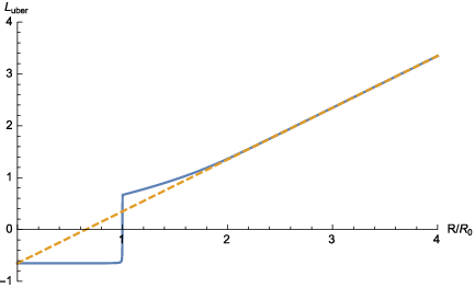
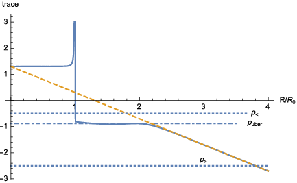
The über-gravity has the following universal properties: i) for high-curvature regime it reduces to the Einstein-Hilbert (EH) action i.e. , ii) for intermediate-curvature regime it predicts a stronger gravity than the EH model, iii) it is vanishing for low-curvature regime () and iv) there is a sharp transition at , which is not sensitive to choice of the basis and parameters [31]. In this sense, über-gravity is a fixed point in the model space which makes it unique. The main goal of this work is to study the cosmology of our model and for this purpose we need to study the equations of motion. However, for our purpose we need the trace of equation of motion (and we assume the case of steady state i.e. is evolving very slowly) which is plotted in Fig. 2.
In the next section, we will introduce a cosmological model based on the general behavior of the über-gravity.
III üCDM cosmology
In this section, we propose a cosmological model which is a natural consequence of über-gravity model. According to Fig. 2, we see that the über-gravity leads to a very simple model for the gravity as
| (5) |
which we call üCDM. In this scenario, if matter density then it sees pure GR with a cosmological constant, while if then the metric is constrained to have constant Ricci scalar i.e. , which is a free parameter in our model presented in Eq.(4). We should mention that the above argument does not depend on the radiation content of the universe since the radiation is trace-free and has no contribution to our conclusion based on Fig. 2.
The sharp transition in our model is representative of a family of models that have different physics for early and late time universe. Such models may address the tensions between early and late time observations. In this sense, our model (5) is very similar to vacuum metamorphosis scenario [34] though they are conceptually different and we do not have any claim about the vacuum structure [35].
In the following sections, we study the background and perturbation of this model.
IV Background Analysis and CMB
The continuity equation for matter gives which means it is decreasing and the universe is in pure CDM phase, i.e. in (5) for early times. Then there is a transition redshift given by when the model switches to phase in (5). For the background we assume a spatially flat FRW metric which gives the following (modified) Friedmann equation for
| (6) |
where and is Hubble parameter at . For we have
| (7) |
where . We assume is continuous at to read from the following relation
| (8) |
Furthermore, we assume continuity of (prime is derivative wrt redshift) or equivalently Ricci scalar which gives us an additional constraint on our parameters
| (9) |
Therefore, we see that üCDM has three independent free parameters i.e. , , and which is one more than standard CDM’s and . Now we are going to constrain üCDM with observational data and contrast it with CDM. To do a fair comparison, we should mention that in the following we will find the best fit of CDM with exactly the same datasets which will be used for üCDM. As such, the best fit values in CDM may be slightly different from those of Planck 2015 [1].
IV.1 Observational Datasets
In the following we report the datasets used in this work including: CMB, local , BAO and Lyman- forest.
| CMB | BAO | BAO | Lyman- | Hubble |
|---|---|---|---|---|
| Planck 2015 [1] | 6dFGS () [39] | LOWZ () [41] | Ly () [10] | Local [3] |
| TTlowP data | ||||
| MGS () [40] | CMASS () [42] | Ly () [10] | ||
For CMB, we use the Planck 2015 TTlowP data [1]. Another data point is given by Riess et al. [3] i.e. km/s/Mpc, and from now on we refer to it by R16. This is the data point which is in tension with Planck 2015 best-fit CDM model. The other dataset is the baryonic acoustic oscillation (BAO) measurements: we use the 6dFGS data at [39], the SDSS main galaxy (MGS) at of [40], Baryon Oscillation Spectroscopic Survey (BOSS) LOWZ [41] at , and CMASS surveys [42] at . To test our model, we consider BAO in Lyman- forest of quasar spectra by [10] who report two independent quantities at ; line of sight distance as and angular distance as where . A tension between Planck 2015 and Lyman- forest BAO has been reported [43] which could potentially be solved with a dynamical dark energy [44]. Here in this work we use the recent analysis [10] which has less tension with Planck 2015. We summarized the datasets in Table 1. In the following, we will report the best fit of our model and standard CDM, with CMB+BAO+R16 which makes our results comparable with Planck 2015 [1].
IV.2 Results
Our results are summarized in Table 2. We contrast best-fit parameters and goodness of fit between üCDM and standard CDM with these datasets 11 1 Note that the best-fit values of CDM may differ slightly from Planck 2015 [1] due to simplified analysis and different dataset combinations.. Also we conduct Akaike information criterion (AIC) to compare the two model with the data set. In Figure (3), we plot the confidence level of standard CDM model in comparison with üCDM, the data set used is CMB+R16+BAO. In Figure (4), we plot the contour plot of the free parameters of üCDM and illustrated the best fits graphically for CMB data set and CMB+BAO+R16. For CDM the best fit values for derived parameters of and km/s/Mpc with . A little bit higher value for in comparison with Planck 2015 [1] is because we have added R16 to our data set which drives a higher value for Hubble parameter (the rest of parameters are listed in Table 2). Our model best fit occurs at km/s/Mpc, and the transition scale factor with . Since üCDM and CDM don’t have the same number of free parameters then analysis may not be very useful. Because of it we have used Akaike information criterion (AIC) analysis [50] which is basically a simplified version of Bayesian analysis and it takes care of the number of free parameters. The AIC results show üCDM is slightly preferred by the datasets even with one more free parameter.
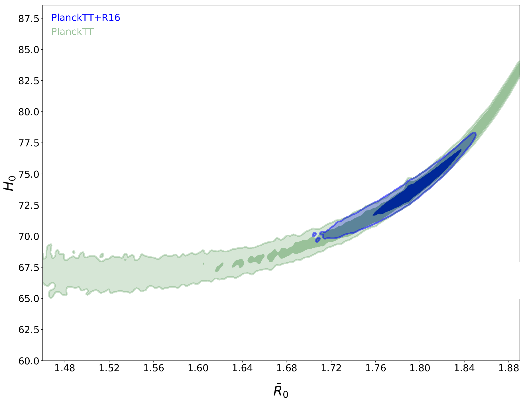
In Fig. 5, we show the confidence level of , and the color-bar showed the value of . This plot also indicates the anti-correlation of the matter density and Hubble parameters, the data set which is used in this plot is CMB+R16+BAO. In Fig. 6, we have the contour plot of and free parameter . This is a crucial plot to compare our results with [51] (see Figure(4) in their paper) which shows the consistency of two models. Green contours shows the constrains from CMB data alone and blue contours obtained from CMB+R16.
We summarize the results in Table 2 and based on these values we plot background distance quantities: In Fig. 7, the angular diameter distance normalized to Planck 2015 best fit values has been plotted. In addition to our distance to the last scattering surface, we plotted the Lyman- forest BAO data point at which shows a 2.5 tension with both models. In Fig. 8, we plotted the volume distance normalized to Planck 2015 best fit values. We have added BAO data and one should compare this plot with Fig. 14 in [1]. In addition to BAO we transformed local measurement [3] to a distance. Planck 2015 and our best-fit CDM model are in tension with R16. However the tension almost disappears in üCDM model, while the tension with Lyman- measurement is reduced.


| CDM | üCDM | |
| Main Parameters | ||
| —– | ||
| Stat. | ||


V Perturbations: the set-up
It is well-known that all theories of gravity can be written as scalar-tensor theories. Consider the following scalar-tensor action representing the cosmological era after the transition in über-gravity:
| (10) |
where is the Ricci scalar, is the trace of the metric , is the (constant) value of curvature after the transition, and is a Lagrange multiplier that is a priori space-time dependent and ensures the constraint . In addition we know from the physics that the above action should be matched with standard CDM which means for it should be standard Einstein-Hilbert action i.e. we should set where is the cosmological constant for . The equations of motion (EOM) for this action are:
| (12) |
The trace of Eq. () can be written using the constraint equation as:
| (13) |
where . Using the results for the linear scalar perturbation of Appendix A we can write the Newtonian potential and lensing potential in the quasi-static regime ():
| (14) | |||
| (15) | |||
| (16) |
where and are the CDM density and peculiar velocity, respectively.
In order to solve Equations (13-16), we first need to know the initial conditions for the fields at . Comparing the action (10) with the Einstein-Hilbert action, we find:
| (17) |
which sets the initial condition for the background equation for in (13). Having solved for , we can plug into Equation (15) to find Newtonian potential, which in turn governs the geodesic equation for CDM. By comparing Equations (15-16) with Einstein equation, we notice that continuity of matter density and velocity implies that there will be a jump in Newtonian potential, while the lensing potential will remain continuous at :
| (18) | |||||
| (19) | |||||
| (20) |
Therefore, the rate of structure formation (at the linear level), which is governed by gravitational acceleration, suddenly jumps by 33% at the onset of the transition. In order to quantify the growth of the structures in linear regime we have to determine the evolution of the growth rate parameter (which is the logarithmic derivative of dark matter density contrast with respect to scale factor). This evolution is governed by the continuity and Euler equation and also the modified Poisson equation which results in
| (21) |
where we should note that the has a dynamic determined from field Einstein field equation as
| (22) |
In Fig.(9) we plot the growth rate versus redshift for CDM and üCDM for two sets of parameters reported in TABLE 2. In addition, we assumed that both constant and evolving (which satisfies (22)) while the background cosmology is governed by üCDM.

In Fig.(10), we plot the growth rate versus dimensionless Hubble parameter, this plot probe a cosmology with expansion history of the Universe and growth rate of perturbations proposed by Linder [52]. The data points of expansion history versus growth rate is from Moresco and Marulli [53].

The real story, of course, is more complicated. Nonlinear structures are already well in place by . Inside haloes and their outskirts, the density never goes below , implying that GR remains valid. The voids, however, could have underdensities of , and thus have crossed over in the über-era, much earlier 22 2 This is a particular extreme of the well-known Chameleon screening [45], which is ubiquitous for generic scalar-tensor theories.. The boost in Newtonian potential can accelerate the emptying of the voids and boost the Integrated Sachs-Wolfe (ISW) effect. Could this provide a means to understand the void phenomenon [11], or the anomalously large ISW effects observed in voids [46] and in general [47]? We defer studying these possibilities to future work, but comment that, due to their nonlinear nature, they can only be satisfactorily addressed using numerical simulations.
VI Concluding remarks
In this work, we show how from the idea of über-gravity a cosmological model is emerged. We call this model üCDM, to indicate two distinct phases of cosmological evolution: The era of CDM, and the über-era with a constant Ricci scalar. The universe is in pure CDM and GR when matter density is larger than a critical density, . After matter density drops below , the universe is in a state with a constant Ricci scalar where we find a suitable solution for Hubble parameter to match the data. This behavior can be seen in a more general context, as a phase transition in gravity, and über-gravity, naturally, provides such a framework to think about such a phase transition. We showed, at the level of background, üCDM can be a potential resolution for the tension between high and low redshift measurements, noting that the measured in local universe is computed in the über-era. We also show that in the level of background the üCDM model fits with the BAO data better than CDM, albeit marginally.
Furthermore, we provide a preliminary analysis of structure formation in üCDM, showing that structure formation will be enhanced in the über-era. This is most likely to affect cosmic voids, and could potentially explain anomalies associated with void structure formation. We plan to study this possibility in the future.
Note-I: Recently, LIGO reported detection of gravity wave from a NS-NS binary with its EM counterpart [48]. By using gravitational wave as standard siren (which is completely independent of SNe or CMB) they could measure Hubble parameter, km/s/Mpc [49], which as of yet cannot distinguish the models discussed here. Higher statistics of such observations can reduce the errors and shed light on the status of tension in cosmology.
Note-II: During the final stages of this work, Valentino, Linder and Melchiorri submitted a preprint that addressed the tension via Parker’s model of Vacuum Metamorphosis (VM) [51] which has a very similar structure to our model. The difference is that they also consider other cosmological parameters beyond CDM to improve the fit, while they do not provide a consistent treatment for perturbations in VM.
Acknowledgments:
We are grateful to P. Creminelli, A.-C. Davis, Mohammad Ali Islami, J. Khoury, Michele Ennio Maria Moresco, S. Rahvar, M. M. Sheikh-Jabbari and R. K. Sheth for insightful comments and discussions. We should thank Hossein Mos’hafi for his extensive discussions on the CMB data analysis part. We also thank the anonymous referee for her/his valuable comments.
SB and NK would like to thank NORDITA workshop on “Advances in theoretical cosmology in light of data”, where this work was initiated there and the Abdus Salam International Center of Theoretical Physics (ICTP) for a very kind hospitality, which the main part of this work has been done there. NK also thanks Perimeter Institute, CITA and Orsay/Saclay (“DarkMod workshop/conference”) for their supports during completion of this work. This research is partially supported by Sharif University of Technology Office of Vice President for Research under Grant No. G960202. NK would like to
thank the research council of Shahid Beheshti University
for their supports.
Appendix A Perturbations
In this section, we derive the background and linearly perturbed EOMs of Eqs. ()-(13). To this end, we expand the EOM to linear order in scalar metric perturbations in the longitudinal gauge:
| (23) | |||||
| (24) | |||||
| (25) | |||||
| (26) | |||||
| (27) |
where . The background EOMs are:
| (28) | |||||
| (29) | |||||
| (30) |
where .
The EOMs at linear order are:
| (31) | |||||
| (32) | |||||
| (33) |
The component of the equation of motion is
| (34) |
And the continuity, Euler equation and the evolution of dark matter density contrast are given accordingly
| (35) |
| (36) |
| (37) |
References
- [1] P. A. R. Ade et al. [Planck Collaboration], “Planck 2015 results. XIII. Cosmological parameters,” Astron. Astrophys. 594, A13 (2016) [arXiv:1502.01589 [astro-ph.CO]].
- [2] M. Tegmark et al. [SDSS Collaboration], “Cosmological parameters from SDSS and WMAP,” Phys. Rev. D 69, 103501 (2004) doi:10.1103/PhysRevD.69.103501 [astro-ph/0310723].
- [3] A. G. Riess et al., “A 2.4 Determination of the Local Value of the Hubble Constant,” Astrophys. J. 826, no. 1, 56 (2016) [arXiv:1604.01424 [astro-ph.CO]].
- [4] A. G. Riess et al.,“New Parallaxes of Galactic Cepheids from Spatially Scanning the Hubble Space Telescope: Implications for the Hubble Constant,” Astrophys. J. 855, no. 2, 136 18 (2018) [arXiv:1801.01120 [astro-ph.SR]].
- [5] A. G. Riess, S. Casertano, W. Yuan, L. M. Macri and D. Scolnic, arXiv:1903.07603 [astro-ph.CO].
- [6] J. L. Bernal, L. Verde and A. G. Riess, “The trouble with ,” JCAP 1610, no. 10, 019 (2016) [arXiv:1607.05617 [astro-ph.CO]].
- [7] T. M. C. Abbott et al. [DES Collaboration], “Dark Energy Survey Year 1 Results: Cosmological Constraints from Galaxy Clustering and Weak Lensing,” arXiv:1708.01530 [astro-ph.CO].
- [8] S. Joudaki et al., Mon. Not. Roy. Astron. Soc. 474, no. 4, 4894 (2018) doi:10.1093/mnras/stx2820 [arXiv:1707.06627 [astro-ph.CO]].
- [9] S. Joudaki et al., Mon. Not. Roy. Astron. Soc. 465, no. 2, 2033 (2017) doi:10.1093/mnras/stw2665 [arXiv:1601.05786 [astro-ph.CO]].
- [10] H. du Mas des Bourboux et al., “Baryon acoustic oscillations from the complete SDSS-III Ly-quasar cross-correlation function at ,” arXiv:1708.02225 [astro-ph.CO].
- [11] P. J. E. Peebles, “The void phenomenon,” Astrophys. J. 557, 495 (2001) doi:10.1086/322254 [astro-ph/0101127].
- [12] A. A. Klypin, A. V. Kravtsov, O. Valenzuela and F. Prada, “Where are the missing Galactic satellites?,” Astrophys. J. 522, 82 (1999) doi:10.1086/307643 [astro-ph/9901240].
- [13] V. Poulin, K. K. Boddy, S. Bird and M. Kamionkowski, Phys. Rev. D 97, no. 12, 123504 (2018) doi:10.1103/PhysRevD.97.123504 [arXiv:1803.02474 [astro-ph.CO]].
- [14] L. Amendola et al., Living Rev. Rel. 21, no. 1, 2 (2018) doi:10.1007/s41114-017-0010-3 [arXiv:1606.00180 [astro-ph.CO]].
- [15] E. J. Copeland, M. Sami and S. Tsujikawa, “Dynamics of dark energy,” Int. J. Mod. Phys. D 15, 1753 (2006) doi:10.1142/S021827180600942X [hep-th/0603057].
- [16] B. Jain and J. Khoury, “Cosmological Tests of Gravity,” Annals Phys. 325, 1479 (2010) doi:10.1016/j.aop.2010.04.002 [arXiv:1004.3294 [astro-ph.CO]].
- [17] T. Clifton, P. G. Ferreira, A. Padilla and C. Skordis, “Modified Gravity and Cosmology,” Phys. Rept. 513, 1 (2012) doi:10.1016/j.physrep.2012.01.001 [arXiv:1106.2476 [astro-ph.CO]].
- [18] E. Di Valentino, A. Melchiorri and O. Mena, “Can interacting dark energy solve the tension?,” Phys. Rev. D 96 (2017) no.4, 043503 doi:10.1103/PhysRevD.96.043503 [arXiv:1704.08342 [astro-ph.CO]].
- [19] W. Yang, S. Pan, E. Di Valentino, R. C. Nunes, S. Vagnozzi and D. F. Mota, “Tale of stable interacting dark energy, observational signatures, and the tension,” arXiv:1805.08252 [astro-ph.CO].
- [20] E. Di Valentino, C. Bøehm, E. Hivon and F. R. Bouchet, “Reducing the and tensions with Dark Matter-neutrino interactions,” Phys. Rev. D 97 (2018) no.4, 043513 doi:10.1103/PhysRevD.97.043513 [arXiv:1710.02559 [astro-ph.CO]].
- [21] S. Nesseris, G. Pantazis and L. Perivolaropoulos, Phys. Rev. D 96 (2017) no.2, 023542 doi:10.1103/PhysRevD.96.023542 [arXiv:1703.10538 [astro-ph.CO]].
- [22] B. Mostaghel, H. Moshafi and S. M. S. Movahed, “Non-minimal Derivative Coupling Scalar Field and Bulk Viscous Dark Energy,” Eur. Phys. J. C 77 (2017) no.8, 541 doi:10.1140/epjc/s10052-017-5085-1 [arXiv:1611.08196 [astro-ph.CO]].
- [23] E. Di Valentino, A. Melchiorri and J. Silk, Phys. Lett. B 761, 242 (2016) doi:10.1016/j.physletb.2016.08.043 [arXiv:1606.00634 [astro-ph.CO]].
- [24] V. Poulin, T. L. Smith, T. Karwal and M. Kamionkowski, “Early Dark Energy Can Resolve The Hubble Tension,” arXiv:1811.04083 [astro-ph.CO].
- [25] A. De Felice and S. Mukohyama, “Graviton mass might reduce tension between early and late time cosmological data,” Phys. Rev. Lett. 118 (2017) no.9, 091104 doi:10.1103/PhysRevLett.118.091104 [arXiv:1607.03368 [astro-ph.CO]].
- [26] A. Banihashemi, N. Khosravi and A. H. Shirazi, arXiv:1810.11007 [astro-ph.CO].
- [27] A. Banihashemi, N. Khosravi and A. H. Shirazi, arXiv:1808.02472 [astro-ph.CO].
- [28] K. Vattis, S. M. Koushiappas and A. Loeb, arXiv:1903.06220 [astro-ph.CO].
- [29] P. Bode, J. P. Ostriker and N. Turok, “Halo formation in warm dark matter models,” Astrophys. J. 556, 93 (2001) doi:10.1086/321541 [astro-ph/0010389].
- [30] N. Khosravi, “Ensemble Average Theory of Gravity,” Phys. Rev. D 94, no. 12, 124035 (2016) [arXiv:1606.01887 [gr-qc]].
- [31] N. Khosravi, “Über-Gravity and the Cosmological Constant Problem,” arXiv:1703.02052 [gr-qc].
- [32] M. Tegmark, “The Mathematical Universe,” Found. Phys. 38, 101 (2008) [arXiv:0704.0646 [gr-qc]].
- [33] N. Arkani-Hamed, T. Cohen, R. T. D’Agnolo, A. Hook, H. D. Kim and D. Pinner, “Solving the Hierarchy Problem at Reheating with a Large Number of Degrees of Freedom,” Phys. Rev. Lett. 117, no. 25, 251801 (2016) [arXiv:1607.06821 [hep-ph]].
- [34] R. R. Caldwell, W. Komp, L. Parker and D. A. T. Vanzella, “A Sudden gravitational transition,” Phys. Rev. D 73, 023513 (2006) doi:10.1103/PhysRevD.73.023513 [astro-ph/0507622].
- [35] A. D. Sakharov, “Vacuum quantum fluctuations in curved space and the theory of gravitation,” Sov. Phys. Dokl. 12, 1040 (1968) [Dokl. Akad. Nauk Ser. Fiz. 177, 70 (1967)] [Sov. Phys. Usp. 34, 394 (1991)] [Gen. Rel. Grav. 32, 365 (2000)].
- [36] Y. Wang and P. Mukherjee, “Robust dark energy constraints from supernovae, galaxy clustering, and three-year wilkinson microwave anisotropy probe observations,” Astrophys. J. 650, 1 (2006) [astro-ph/0604051].
- [37] O. Elgaroy and T. Multamaki, “On using the CMB shift parameter in tests of models of dark energy,” Astron. Astrophys. 471, 65 (2007) [astro-ph/0702343 [ASTRO-PH]].
- [38] E. Komatsu et al. [WMAP Collaboration], “Five-Year Wilkinson Microwave Anisotropy Probe (WMAP) Observations: Cosmological Interpretation,” Astrophys. J. Suppl. 180, 330 (2009) [arXiv:0803.0547 [astro-ph]].
- [39] F. Beutler, C. Blake, M. Colless, D. H. Jones, L. Staveley-Smith, L. Campbell, Q. Parker, W. Saunders and F. Watson, “The 6dF Galaxy Survey: Baryon Acoustic Oscillations and the Local Hubble Constant,” Mon. Not. Roy. Astron. Soc. 416, no. 4, 3017 (2011) [arXiv:1106.3366 [astro-ph.CO]].
- [40] A. J. Ross, L. Samushia, C. Howlett, W. J. Percival, A. Burden and M. Manera, “The clustering of the SDSS DR7 main Galaxy sample I. A 4 per cent distance measure at ,” Mon. Not. Roy. Astron. Soc. 449, no. 1, 835 (2015) [arXiv:1409.3242 [astro-ph.CO]].
- [41] L. Anderson et al. [BOSS Collaboration], “The clustering of galaxies in the SDSS-III Baryon Oscillation Spectroscopic Survey: baryon acoustic oscillations in the Data Releases 10 and 11 Galaxy samples,” Mon. Not. Roy. Astron. Soc. 441, no. 1, 24 (2014) [arXiv:1312.4877 [astro-ph.CO]].
- [42] H. Gil-Marín et al., “The clustering of galaxies in the SDSS-III Baryon Oscillation Spectroscopic Survey: BAO measurement from the LOS-dependent power spectrum of DR12 BOSS galaxies,” Mon. Not. Roy. Astron. Soc. 460 (2016) no.4, 4210 [arXiv:1509.06373 [astro-ph.CO]].
- [43] A. Font-Ribera et al. [BOSS Collaboration], “Quasar-Lyman Forest Cross-Correlation from BOSS DR11 : Baryon Acoustic Oscillations,” JCAP 1405, 027 (2014) [arXiv:1311.1767 [astro-ph.CO]].
- [44] G. B. Zhao et al., “Dynamical dark energy in light of the latest observations,” Nat. Astron. 1, 627 (2017) [arXiv:1701.08165 [astro-ph.CO]].
- [45] J. Khoury and A. Weltman, “Chameleon fields: Awaiting surprises for tests of gravity in space,” Phys. Rev. Lett. 93, 171104 (2004) doi:10.1103/PhysRevLett.93.171104 [astro-ph/0309300].
- [46] A. Kovcs, “The part and the whole: voids, voids, and their ISW imprint,” arXiv:1701.08583 [astro-ph.CO].
- [47] S. Ho, C. Hirata, N. Padmanabhan, U. Seljak and N. Bahcall, “Correlation of CMB with large-scale structure: I. ISW Tomography and Cosmological Implications,” Phys. Rev. D 78, 043519 (2008) doi:10.1103/PhysRevD.78.043519 [arXiv:0801.0642 [astro-ph]].
- [48] B. P. A. et. al. (LIGO Scientific Collaboration and Virgo Collaboration), “GW170817: Observation of Gravitational Waves from a Binary Neutron Star Inspiral,” Phys. Rev. Lett. 119, 161101 (2017).
- [49] B. P. Abbott et al. [The LIGO Scientific and The Virgo and The 1M2H and The Dark Energy Camera GW-EM and the DES and The DLT40 and The Las Cumbres Observatory and The VINROUGE and The MASTER Collaborations], “A gravitational-wave standard siren measurement of the Hubble constant,” Nature doi:10.1038/nature24471 [arXiv:1710.05835 [astro-ph.CO]].
- [50] H. Akaike, IEEE Trans. Autom. Control 19, 716 (1974). doi:10.1109/TAC.1974.1100705.
- [51] E. Di Valentino, E. Linder and A. Melchiorri, “A Vacuum Phase Transition Solves Tension,” arXiv:1710.02153 [astro-ph.CO].
- [52] E. V. Linder, “Cosmic Growth and Expansion Conjoined,” Astropart. Phys. 86, 41 (2017) doi:10.1016/j.astropartphys.2016.11.002 [arXiv:1610.05321 [astro-ph.CO]].
- [53] M. Moresco and F. Marulli, “Cosmological constraints from a joint analysis of cosmic growth and expansion,” Mon. Not. Roy. Astron. Soc. 471, no. 1, L82 (2017) doi:10.1093/mnrasl/slx112 [arXiv:1705.07903 [astro-ph.CO]].