Multi-Objective Approaches to Markov Decision Processes with Uncertain Transition Parameters
Abstract.
Markov decision processes (MDPs) are a popular model for performance analysis and optimization of stochastic systems. The parameters of stochastic behavior of MDPs are estimates from empirical observations of a system; their values are not known precisely. Different types of MDPs with uncertain, imprecise or bounded transition rates or probabilities and rewards exist in the literature.
Commonly, analysis of models with uncertainties amounts to searching for the most robust policy which means that the goal is to generate a policy with the greatest lower bound on performance (or, symmetrically, the lowest upper bound on costs). However, hedging against an unlikely worst case may lead to losses in other situations. In general, one is interested in policies that behave well in all situations which results in a multi-objective view on decision making.
In this paper, we consider policies for the expected discounted reward measure of MDPs with uncertain parameters. In particular, the approach is defined for bounded-parameter MDPs (BMDPs) (Givan et al., 2000). In this setting the worst, best and average case performances of a policy are analyzed simultaneously, which yields a multi-scenario multi-objective optimization problem. The paper presents and evaluates approaches to compute the pure Pareto optimal policies in the value vector space.
1. Introduction
Markov decision processes (MDPs) are a common tool to describe decision situations in many different contexts such as performance optimization and planning (Puterman, 1994; Bertsimas et al., 2016; Bertsimas and Mišić, 2017; Kolobov, 2012). The general idea is to specify a system by means of different states in which it can be, actions which a decision maker can perform to affect the (probabilistic) future behavior, and rewards or costs that depend on the state and decision such as energy costs of a server starting up or the amount of users served in a queue if a service is active. After an action has been chosen, the system changes its state depending on the action and the current state but not on the past behavior; transitions are, in general, randomized and defined by the system’s properties.
However, modeling a physical or an artificial system suffers from several limitations. Most prominent is the inherent loss of precision that is introduced by measurement errors and discretization artifacts which necessarily happen due to incomplete knowledge about the system behavior. So the true probability distribution to be associated with transitions is in most cases uncertain and instead can be given by either external parameters or confidence intervals. To account for the latter, the MDP model has been extended to bounded-parameter MDPs (BMDPs) (Givan et al., 2000) or the slightly more general classes of MDPs with incomplete or uncertain transition probabilities (Satia and Lave, 1973; White and Eldeib, 1994). In these classes of MDPs, best-case and worst-case policies for expected discounted reward measures have been considered. These policies result in upper and lower bounds for the value vector that contains the discounted accumulated reward gained after starting in the different states of the process.
Robust optimization techniques (Wiesemann et al., 2013) are useful to derive policies that hedge against model uncertainties. In particular, these robust policies optimize the expected discounted reward against the worst possible realization of the uncertainty. From the viewpoint of a potential decision maker, however, a robust solution may be overly pessimistic. A decision maker is often interested in a solution that might be not fully robust, but instead could have an acceptable worst-case behavior while retaining good best-case and average-case (for a properly defined concept of “average”) performance. This property may be formalized in several alternative ways; most notably, there are several competing definitions of “almost robust” solutions (Klamroth et al., 2013). A further optimization goal in this context may be the probability of reaching a certain performance bound, assuming some probability distribution over the uncertainty set. Unfortunately, the latter seems to be inherently hard, especially for uncertain MDPs (Scheftelowitsch, 2015).
Thus a promising approach considers not only one extremal measure (either the upper or the lower bound), but at least both bounds, and possibly the expectation, and optimizes all of them simultaneously. This means doing multi-objective optimization which yields several mutually incomparable, so-called non-dominated policies for the uncertain MDP from which the user may select the one which has the most suitable performance measures. This may be in particular of interest if the differences between the optimal policies in the different scenarios are sufficiently large to consider different tradeoffs besides the obvious extremal points. In this paper, we develop methods to compute all pure non-dominated policies for a given uncertain MDP in a specific uncertainty setting which can be generalized to other notions of parameter uncertainty. This problem which is basically an instance of multi-scenario optimization asks to compute policies which are optimal in the presence of trade-offs between several conflicting objectives.
It is worthwhile to mention that for the considered multi-objective optimization problem, the number of optimal, i.e., mutually incomparable and non-dominated solutions may be exponentially high, which is a structural feature of the problem, and computing all of these solutions might take a prohibitive amount of time. However, for “stationary” decision-making problems which only rarely vary with time, we argue that the amount of time invested in finding an optimal policy is often negligible when compared to the actual performance of the policy implementation.
Related work. The Bounded-parameter MDP (BMDP) model is introduced and widely discussed in (Givan et al., 2000). BMDPs are a specific subclass of MDPs with uncertain or imprecise transition probabilities proposed by (Satia and Lave, 1973) and (White and Eldeib, 1994). The methods extend to more general notions of uncertainty in MDPs such as convex uncertainty sets discussed by (Puggelli et al., 2013); further aspects of parameter uncertainty in MDPs are covered in (Delgado et al., 2011; Wiesemann et al., 2013; Iyengar, 2005). However, in almost all cases, the goal is to compute a robust policy which ensures the best possible behavior in the worst case. In many scenarios however, we may have a multidimensional reward function and hence search for a policy which simultaneously maximizes all reward dimensions. To account for the latter, multi-objective Markov decision processes are discussed in (Wiering and de Jong, 2007; White, 1982; Chatterjee et al., 2006; Barrett and Narayanan, 2008; Perny and Weng, 2010). The extension to multi-objective Markov decision processes under bounded parameter uncertainty has recently been investigated in (Hahn et al., 2017). In this paper, we target another facet of multi-objective multi-scenario optimization for MDPs with parameter uncertainty where the goal is to simultaneously optimize the worst, best and average case behavior.
There exist numerous applications of MDPs and uncertainty modeling in the performance optimization world. They include decision support in medical screening procedures (Bertsimas et al., 2016) and product line design (Bertsimas and Mišić, 2017). Applications and the general formulation of multi-scenario optimization are given in (Wiecek et al., 2009).
Our Contribution. This work considers the multi-scenario multi-objective optimization problem for BMDPs where the multiple scenarios correspond to the maximal, minimal, and average performance measures of a given policy in the uncertainty set of BMDPs. The notion of average performance is given by slightly extending the existing BMDP formalism and defining a designated average MDP in the uncertainty set. In particular, we define the average MDP by introducing a probability distribution over the uncertainty set and deriving the expected value. This has the advantage of possible further applications such as percentile optimization.
In summary, the main contributions of this paper are threefold. First, we provide an exact algorithm that computes the desired set of pure Pareto optimal policies, albeit at a (almost certainly) prohibitively high computational cost. Second, we design a heuristic that is efficient in the sense that it computes a set of mutually non-dominated policies that are likely to be Pareto optimal with reasonable time complexity. Finally, we develop a prototype tool and apply it to some case studies to show the effectiveness of our approach.
2. Mathematical Preliminaries
We start with common notations and formalisms used in this paper.
For a matrix , we denote by the entry in row and column . Vector identifiers, such as , appear in bold script, to distinguish them from scalars and matrices. For a natural number , we designate by the set . For multi-dimensional identifiers, such as matrices or vectors, the order relations or are performed componentwise. Additionally, we define to be short for .
We next motivate and formally introduce the modelling formalism considered in this paper.
In a Markov decision process, transition probabilities and rewards are estimates resulting from measurements or expert opinion. This implies that there is always uncertainty about the parameters of the model and also about the behavior of the real system according to some policy that has been derived from the MDP. The class of stochastic bounded-parameter MDPs (SBMDPs) includes this uncertainty by considering intervals rather than point estimates for the parameters of MDPs and defining a probability distribution over the uncertainty set. We shall use the probability distribution in order to derive the “average” MDP and then work with this MDP; for the sake of generality, we would like to define the formalism here completely with the probability distribution.
Definition 2.1 (Stochastic bounded-parameter Markov process).
A stochastic bounded-parameter Markov decision process (SBMDP) is a tuple where is a (finite) state space, is a (finite) set of actions, is a set of matrix pairs where for each , , , is a set of reward vector pairs where for each , and is a probability measure on the rewards and the transition matrices for each action.
We denote by all vectors such that for all and . Similarly specifies all vectors such that .
It is worthwhile to note that the model of SBMDPs extends the formalism of BMDPs introduced by (Givan et al., 2000) with a probability measure on the possible transition matrices and reward vectors, so as to enable to take the “average performance” into consideration by deriving expected values for the transition matrices and rewards. This is different from the expected value of the value vector under the probability distribution, as here the expectation operator is applied on the model and serves to define an additional optimization objective, in addition to the upper and lower bounds for the value vectors.
To optimize the performance of a (SB)MDP, a decision rule or policy is needed. Formally, a policy is a function where is the set of (finite) histories of states and is the set of probability distributions on . We call a policy pure if it is stationary, i.e., it depends only on the current state, and deterministic, i.e, it always maps a history to a Dirac distribution, i.e., . We use for general policies and for stationary and pure policies. We denote by the action that is chosen in state using policy , if is pure.
Moreover, a stationary policy induces a Markov reward process with transition matrix and reward vector . For a transition matrix and state , we denote by the -th row of . Accordingly, we denote by the -th row of and by the reward of state under policy . For pure policies, we define a Hamming distance measure by .
The expected discounted reward for an infinite horizon is taken as performance metric. For a MDP, a given policy defines a sequence of transition matrices and reward vectors where resp. is the transition matrix resp. the reward in the -th time step. Using this sequence, we derive a probability distribution on sequences of states and corresponding rewards, from which the expected discounted reward is defined by .
A value vector collects the computed expected discounted reward for all states where each entry equals the expected discounted reward one obtains starting from the respective state. The mathematical properties of expected discounted rewards on which we shall rely in the sequel are widely discussed by (Puterman, 1994).
We assume that the goal is the maximization of the expected discounted reward. For a SBMDP policies assuring best and worst case behavior can be determined by solving the following Bellman equations for the value vectors .
| (1) |
As shown by (Givan et al., 2000), the optimal policies are pure. We denote them by and , respectively.
Additionally, we are interested in the “average-case” properties of SBMDPs and a policy that maximizes the performance under the “average-case” assumption. The reasoning here is fairly straightforward: Since the probability distribution for the transition matrices is known, we can define for each action , and , where are probability densities on transition matrices and reward vectors for action . The Bellman equations become
| (2) |
which is a standard MDP problem. The optimal policy is pure and is denoted as . For a policy , by , and we designate the lower, upper and average value vectors, furthermore, the triple is designated by , if not mentioned otherwise. Obviously and also hold, as and are the minimal resp. maximal value vectors for over all MDPs in the uncertainty set. Usually , , and differ and a compromise between two or all three goals has to be found.
Before we discuss specifics, we would like to mention a possible alternative approach in this setting. It is possible to consider the SBMDP formalism in a Bayesian setting, where the information from the probability distribution over the uncertainty set of MDPs is taken into account completely, thus seeking for where is the value vector of the policy in the MDP . This approach can be undertaken in the case where it is possible to integrate over the probability distribution over easily.
Here, we explicitly choose the multi-objective approach mainly for the reason of larger applicability. Even if a Bayesian approach can be motivated from the standpoint of stochastic BMDPs, one can easily see that any reasonably good solution in the multi-objective setting can be transferred to “plain” BMDPs and, furthermore, to multi-objective MDPs even without introducing a probability distribution over the uncertainty set.
As we shall consider multi-objective optimization problems, we define the set of solutions that interest us.
Definition 2.2 (Pareto Optimality).
Let be the set of pure policies , then we define the Pareto frontier as
the set of pure policies that result in Pareto optimal value vectors. We denote by and the corresponding sets of value vectors.
It is easy to see that holds and usually, the subsets are proper. For convenience, we shall use an operator that operates on sets with a partial order and is defined by .
3. Computation of Optimal Policies
The computation of Pareto optimal policies in multi-objective MDPs is challenging as the number of optimal policies can be large or even infinite (for non-stationary policies). Therefore, algorithms are required to approximate the Pareto set efficiently instead of computing the whole set of Pareto optimal policies. Several works have already explored methods to compute or approximate the Pareto set, e.g., (Perny and Weng, 2010; Barrett and Narayanan, 2008; Chatterjee et al., 2006; White, 1982; Wiering and de Jong, 2007; Roijers et al., 2014) albeit for the computation of several expected values or in a setting that has only a multi-objective reward. In SBMDPs we have to face optimization of, ultimately, several MDPs with related but not identical transition probabilities; furthermore, we consider the worst and best case vectors. This seems to be a different, and generally harder problem.
For most non-trivial models the number of Pareto optimal policies is still much too large to compute them all and many policies show a similar behavior. From a practical point of view it is sufficient to compute a subset of the Pareto frontier if the corresponding value vectors are evenly distributed in the value vector space. Theoretically, one can try value iteration or policy iteration-based approaches to compute policies from and the corresponding value vectors from , as in (Wiering and de Jong, 2007). The disadvantage of value iteration algorithms is that the number of intermediate partly evaluated policies can become enormous before the value iteration converges and the policies get completely evaluated. In this case, one has to stop the algorithm with a large number of non-comparable policies which might even not be optimal since value iteration provided only an approximation or a lower bound of the true value vectors. Thus, we consider a policy iteration-based approach.
In the following, we present two algorithms. The first algorithm computes exactly, albeit at a possibly high computational cost. The second algorithm is a fixed-point iteration that computes an increasing set of mutually non-dominating policies. Our first approach relies on the following result.
Lemma 3.1.
Let be a SBMDP. Let furthermore be two policies where lies on the Pareto frontier. Then there exists a finite sequence of policies where and, additionally, .
From this result, we develop a procedure that computes as sketched in Algorithm 1. Intuitively, the algorithm generates for each currently considered policy possible non-dominated neighbor policies and updates a global set of non-dominated policies. This continues for steps.
Theorem 3.2.
Algorithm 1 correctly computes .
The complexity of the exact algorithm is, as of yet, unclear. In the worst possible case the algorithm will produce large numbers of temporarily optimal policies that will be dominated by a few Pareto-optimal policies in the end, making the worst-case complexity , theoretically independent of the final size of . To avoid this, we propose a slightly different algorithm that computes a set of policies that seem to be a reasonably good approximation of . It is important to note that the following approach is an heuristic; later, we shall discuss the (empirical) quality of this heuristic.
The heuristic approach is a simplification of the Algorithm 1. The simplification lies in including only those policies into the non-dominated set that are non-dominated with respect to all other policies. This decreases the number of candidate policies and, thus, the runtime at the cost of possible inaccuracy.
The practical implementation tries to find quickly policies that are spread over the Pareto frontier by analyzing first those policies which are likely to belong to the Pareto frontier. It is known that the policies belong to , as no other policy has a greater value vector in the lower bound, average, and upper bound case, respectively, by definition. Starting with these policies makes the algorithm walk through the policy space from the extreme points of the Pareto frontier which, as we hope, yields an evenly distributed non-dominated set of policies.
The following simple observation helps to find good policies which are candidates for the Pareto frontier without too many policy evaluations. Let for a policy and a state-action pair the gradient be
| (3) | ||||
If, for some policy , a state and an action can be found such that
| (4) |
then a policy can be defined with for and and for it is . We define an operator
that generates a new policy from by selecting for each the lexicographically smallest action that observes (4), whenever this is possible. Looping until convergence, which occurs in the repeat-loop in lines 14–17, yields a locally optimal policy in the Pareto frontier.
The function considers only pairs where the gradient is positive in all components, making dominate . In fact, the gradient gives a hint how the new policy will behave. From the gradient, the direction of the different value vectors of a new policy can be estimated without evaluating it. Policy evaluation is done by a function eval which solves the following three sets of equations to compute the value vectors for some pure policy .
| (5) | |||
The equations for the average values define a set of linear equations which can be solved with standard techniques. For the vector of the worst and best case an iterative approach is applied: The vectors are successively computed by solving the LP and optimizing the matrix until convergence (Givan et al., 2000).
In our algorithm we use a set that contains tuples . Additionally, we use a set where all evaluated policies are stored to avoid re-evaluations of policies. In the current description, new policies are generated starting from available policies by maximizing one direction of the gradient. The algorithm stops if in the current set of non-dominated policies, the neighbors of each policy are either explored or dominated. A further stopping condition is to explore a predefined number of policies.
As the algorithm is a heuristic, it is difficult to argue about guaranteed performance in terms of quality of the output, that is, if the resulting policies fulfill and . It is still possible to make several observations. The main difference between Alg. 2 and Alg. 1 lies in the bookkeeping that disallows Alg. 2 to explore policies that have been already evaluated and, more importantly, are dominated by some other policy that has been found. By doing this, Alg. 2 may ignore policies that are dominated yet lead (by choosing an appropriate sequence of policy changes) to the Pareto frontier; if there are no other ways to the Pareto frontier, this makes the output of Alg. 2 incomplete. On the other hand, one can provide a heuristic argument: Since the initial set of policies contains known “extreme points” , the policies that will be found by Alg. 2 in realistic settings will stem from a gradual transition from one extreme policy to another, as there will always exist a path of policies that improves one of the objectives until an optimum is reached. This way, we can expect that in real-life problems, the resulting set will cover the Pareto frontier or at least the space between the value vector tuples adequately, i. e., the resulting set of value vectors will be evenly distributed in the space between the extreme value vectors stemming from . Furthermore, we expect that for practical problems, the following assumption will hold: If for a set of policies it is and contains not all Pareto optimal policies, then there exists a policy and a state-action pair such that and is not dominated by any other policy in . This especially means that there is always a “globally” non-dominated path of policies from a set of mutually non-dominating policies to a policy in if . We expect that this assumption holds for practical instances. Furthermore, we conjecture that our assumption is also true for the problem in general. Finally, since Algorithm 2 is a variation of Algorithm 1, the same complexity reasoning applies here. However, the practical complexity should be lower than that of Algorithm 1, as less SBMDP evaluations have to be performed.
4. Evaluation
We have performed a series of experiments where we considered several questions. First, we compared the performance of Algorithm 2 against a black-box multi-objective optimization method as reference. We have chosen SPEA2 (Zitzler et al., 2001) as reference since it is a well-studied, simple black-box optimization algorithm. Second, we have evaluated the general performance of the algorithm with respect to problem size and the number of computed solutions.
For the evaluation, we have used a machine with an Intel® Core™ i7-4790 CPU and RAM. We have set a time limit of for SPEA2 and a limit for Algorithm 2 of checked policies. The archive size for SPEA2 has been set to . Concerning the implementations, we have used OpenMP parallelization methods to use multiple CPU cores when possible. Furthermore, we have used advanced numerical algorithms to evaluate (1) and (2). Specifically, for large instances, we substituted the direct LU solver (Stewart, 1994) by preconditioned GMRES (Saad, 1993; Stewart, 1994) with an ILU0-preconditioner. The code and testing infrastructure are available at (Scheftelowitsch and Buchholz, 2016) and (Scheftelowitsch, 2016).
4.1. The Model of Multi-Server Queue
As the first case study, we have chosen a parameterizable model that can be easily generated; more concretely, we have considered a multi-server queue where servers can be switched off to save energy and switched on if the load in the system increases. Such queues are abstract models for server farms (Gandhi et al., 2010). The goal is to find a compromise between small response times and low energy consumption.
We consider a system where customers arrive according to a Poisson process with rate and require an exponentially distributed service with mean . As our algorithms are designed for discrete-time BMDPs, we consider a (morally) equivalent discrete model where the probability of arrival of a customer in a time unit is , the service probability is and, thus and are multiples of resp. . The system has a capacity of and contains servers. Each server can be in one of three states on, off and start. A server can be switched off after the end of a service or if it is idle. A server that is switched off immediately changes its state from on to off. Servers in state off can be switched on which means that they change their state to start. The duration of the starting period is exponentially distributed with rate , then the server changes its state to on and is ready to serve customers. A state of the system can be described by where describes the number of customers, include the number of servers in state on, start and off, respectively. Consequently, has to hold. The number of states equals . The reward in the state equals where , describe the energy consumption in the on, start, and off state.
The upper and lower bounds for the transition probabilities were chosen randomly by generating Gaussian noise and adding it to the transition probabilities defined above.
Comparison to a generic heuristic.
As we consider a new problem, we have chosen to compare our approach to a black-box heuristic. More specifically, we have considered multi-objective optimization heuristics and decided to compare our algorithm to SPEA2 as it is a well-studied evolutionary optimization algorithm that is specifically designed to compute non-dominated sets for multi-objective optimization problems.
The SPEA2 algorithm. In detail, SPEA2 keeps two sets: a population and an archive where the non-dominated solutions are stored. In each iteration of the optimization cycle, is updated with non-dominated elements of . Then, a selection step takes place in which first, all elements of are assigned a fitness value and then, the solutions with lower fitness values are chosen to generate new solutions by application of mutation and crossover operators. The newly generated solutions are then the new population.
The distinctive feature of this approach is the fitness evaluation: The fitness of an individual solution depends on the strength of other solutions that cover . The strength itself is defined as the number of covered solutions; thus, the non-dominated solutions have maximal strength and minimal fitness values by definition, otherwise the ranking aims at picking more diverse solutions, i. e., solutions that are more evenly distributed in the objective value space.
In our SPEA2 implementation,we have defined problem-specific mutation and crossover operators. As possible solutions are stationary policies, the operators could be defined in a straightforward fashion. Mutation affects a decision in one state with probability , if is the number of states in the MDP, and replaces the previous action in the policy with a random one. Crossover takes two “parent” policies and chooses for the result an action from either of the original policies with probability .
Comparison metrics. To quantify performance differences, we have used the coverage metric that has been introduced in (Zitzler and Thiele, 1999). This performance metric has been designed to compare two output sets of (heuristic) multi-objective optimization algorithms on the same problem and computes the fraction of one output that is covered (i. e., is dominated by or equal to) by an element of the other output set. Concretely, for two sets of vectors and , the coverage metric is defined by . means that all points in are dominated by or equal to points in whereas means that no point in is covered by a point in . It is worth noting that the coverage metric is asymmetric and in most cases it is interesting to compute both and .
Results. The results of the comparison can be found in Fig. 1. The first figure describes the coverage metric where the first argument is the policy set computed by Alg. 2, the second figure describes the converse. In the run, SPEA2 took always while Alg. 2 did never take more than .


It is easy to see that Algorithm 2 almost always delivers a significantly better performance with respect to both time complexity as well as quality of computed policies. More concretely, in nearly all cases Algorithm 2 has computed a set that completely covered all solutions generated by SPEA2; the evolutionary heuristic, however, has never produced a policy that strictly dominated a policy from Alg. 2 and was only able to yield comparable solutions on small instances with state space size of at most .
Comparison to an exact computation.
For some instances, we have furthermore compared the performance of Algorithm 2 to the exact approach in Algorithm 1. Concretely, we have considered the case . It has turned out that for this case, the coverage metric was always . This suggests that Algorithm 2 may compute the complete Pareto frontier not only heuristically but also in theory. This is, however, a conjecture subject to further investigation.
4.2. Time complexity measurements
As the number of policies was bounded by an upper limit of and , the complexity can be roughly estimated by a cubic term in . For practical applications, we are also interested in runtimes on real-life instances. For this, we have used a slightly different but more general (and somewhat more scalable) model.
The grid model. We have chosen a model that resembles a grid with states and actions . The rewards for actions in each state are chosen randomly with mean and variance . The transition probabilities are also chosen randomly according to the Dirichlet distribution. Concretely, the transition probability vector from state to states for action is Dirichlet-distributed with concentration parameters where if and otherwise which yields an (expected) 10 times larger probability to land in than in other states. The upper and lower bounds are, as before, generated by adding Gaussian noise.
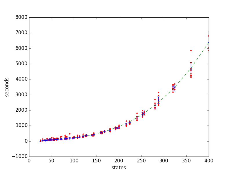
Complexity. We present the results in graphical form. To get the results, we have run Algorithm 2 on instances with up to states, with and between 5 and 20. For each , we have created instances.
The results can be seen in Fig. 2(a) and Fig. 2(b). The red dots are the empirical data, the blue lines describe a confidence interval that stems from a (scaled) t-distribution guess. The green line is the cubic regression term for convenience. One can see that the experimental performance generally matches a polynomial term, but also that even on large instances, the mean time until a non-dominated solution is generated lies under a second.

4.3. The Model of Autonomous Nondeterministic Tour Guides
Our second case study is inspired by “Autonomous Nondeterministic Tour Guides” (ANTG) in (Cantino et al., 2007; Hashemi et al., 2016), which models a complex museum with a variety of collections.
Models in (Cantino et al., 2007) are MDPs. In our experiment, we will insert some uncertainties into the MDP. Due to the popularity of the museum, there are many visitors at the same time. Different visitors may have different preferences of arts. We assume the museum divides all collections into different categories so that visitors can choose what they would like to visit and pay tickets according to their preferences. In order to obtain the best experience, a visitor can first assign certain weights to all categories denoting their preferences to the museum, and then design the best strategy for a target. However, the preference of a sort of arts to a visitor may depend on many factors like price, weather, or the length of queue at that moment etc., hence it is hard to assign fixed values to these preferences. In our model we allow uncertainties of preferences such that their values may lie in an interval.
For simplicity we assume all collections are organized in an square with . Let . We assume all collections at are assigned with a weight 1 if or , with a weight 2 if or ; otherwise they are assigned with a weight interval . In other words, we expect collections in the middle will be more popular and subject to more uncertainties than others. Furthermore, we assume that people at each location have two non-deterministic choices: either move to the north and east, that is, or to the north and west, that is, if , while if , they can move either to the north and east, , or to the south and east, that is, . The transitions also depend on the location of the collection. For the collections in the middle, the main direction of transition is chosen with probability while the probability to move to some other neighbor collection is . In the expected case, we set the probability to move to the collection in the main direction to and distribute the remaining probability mass evenly among other neighbor collections. For collections outside the middle, the main direction (for example, north and west) is chosen with probability .
Therefore a model with parameter has states in total and roughly transitions, 2% of which are associated with uncertain weights and uncertain transition probabilities. Notice that a transition with uncertain weights essentially corresponds to several transitions with concrete weights.
We define a reward structure denoting the reward one can obtain by visiting each collection. For simplicity, we let the reward be the same as the weight of a collection. We can ask for the optimal policy for the expected discounted reward criterion, that is, in the scenario where it is preferable to make better rewarding moves early.
Evaluation of the ANTG model
We have performed an evaluation of the model for , with the results depicted in Fig. 3. For convenience, the runtime and the number of policies are plotted in dependence of the number of states, which is . We see that on large instances, the problem structure yields a large number of optimal policies, thus decreasing performance. On small instances, however, the number of optimal policies generated is small, which allows for a fast computation of the Pareto frontier.
5. Conclusions
In this paper, we have presented a novel approach to analyze bounded-parameter Markov decision processes. In contrast to known approaches (Givan et al., 2000) that usually analyze the worst case behavior and result in a variant of robust optimization, the problem is handled here as a multi-objective problem. Of course, the price for this extension can be an exponential complexity due to an exponential number of optimal and mutually incomparable policies in this case. The problem differs from many other multi-objective optimization approaches for MDPs where several expected values are analyzed, whereas here worst, expected and best case behavior are considered together which together yields a multi-scenario optimization problem.
In order to find all Pareto optimal policies in multi-objective optimization of BMDPs, two computational algorithms are presented. One of the algorithms computes the desired set of policies exactly, but has a prohibitive runtime complexity. The second algorithm that is explicitly designed for the problem is a heuristic and seems to perform well on a large number of test instances. In particular, we have shown that the policies obtained by the heuristic were in almost all cases better than those produced by a generic evolutionary multi-objective optimization algorithm.
The approach presented here can be extended in various directions. As mentioned it is fairly easy to consider additional goals beyond worst, average and best cases. Our results not only apply to bounded-parameter Markov decision processes, but can also be utilized for Markov decision processes with convex uncertainties (Puggelli et al., 2013). Therefore, the same basic algorithms can be used in order to compute Pareto optimal policies, if one adjusts them to solve the convex program in the iteration step.
For future research, it would be interesting to consider the stochastic multi-scenario problem for stochastic BMDPs. There, the goal is to optimize the expected value of the value vector, in contrast to the value vector of the expected MDP we have used here. This problem is a slightly different, single-objective optimization problem and needs to be considered separately.
Acknowledgments
This work is supported by the DFG as part of RTG 1855 and by the ERC Advanced Grant 695614 (POWVER).
References
- Barrett and Narayanan (2008) Leon Barrett and Srini Narayanan. 2008. Learning All Optimal Policies with Multiple Criteria. In ICML. 41–47.
- Bertsimas and Mišić (2017) Dimitris Bertsimas and Velibor V. Mišić. 2017. Robust Product Line Design. Operations Research 65, 1 (2017), 19–37. https://doi.org/10.1287/opre.2016.1546
- Bertsimas et al. (2016) Dimitris Bertsimas, John Silberholz, and Thomas Trikalinos. 2016. Optimal healthcare decision making under multiple mathematical models: application in prostate cancer screening. Health care management science (2016), 1–14.
- Cantino et al. (2007) Andrew S. Cantino, David L. Roberts, and Charles L. Isbell. 2007. Autonomous nondeterministic tour guides: improving quality of experience with TTD-MDPs. In AAMAS. IFAAMAS, 22.
- Chatterjee et al. (2006) Krishnendu Chatterjee, Rupak Majumdar, and Thomas A. Henzinger. 2006. Markov Decision Processes with Multiple Objectives. In STACS. 325–336.
- Delgado et al. (2011) Karina Valdivia Delgado, Scott Sanner, and Leliane Nunes de Barros. 2011. Efficient solutions to factored MDPs with imprecise transition probabilities. Artif. Intell. 175, 9-10 (2011), 1498–1527.
- Gandhi et al. (2010) Anshul Gandhi, Mor Harchol-Balter, and Ivo J. B. F. Adan. 2010. Server farms with setup costs. Perform. Eval. 67, 11 (2010), 1123–1138.
- Givan et al. (2000) Robert Givan, Sonia M. Leach, and Thomas L. Dean. 2000. Bounded-parameter Markov decision processes. Artif. Intell. 122, 1-2 (2000), 71–109.
- Hahn et al. (2017) Ernst Moritz Hahn, Vahid Hashemi, Holger Hermanns, Morteza Lahijanian, and Andrea Turrini. 2017. Multi-objective Robust Strategy Synthesis for Interval Markov Decision Processes. CoRR abs/1706.06875 (2017). http://arxiv.org/abs/1706.06875
- Hashemi et al. (2016) Vahid Hashemi, Holger Hermanns, and Lei Song. 2016. Reward-Bounded Reachability Probability for Uncertain Weighted MDPs. In International Conference on Verification, Model Checking, and Abstract Interpretation. Springer, 351–371.
- Iyengar (2005) Garud N. Iyengar. 2005. Robust Dynamic Programming. Mathematics of Operations Research 30, 2 (2005), 257–280.
- Klamroth et al. (2013) K. Klamroth, E. Köbls, A. Schöbel, and Chr. Tammer. 2013. A unified approach for different concepts of robustness and stochastic programming via non-linear scalarizing functionals. Optimization 62, 5 (2013), 649–671.
- Kolobov (2012) Andrey Kolobov. 2012. Planning with Markov decision processes: An AI perspective. Synthesis Lectures on Artificial Intelligence and Machine Learning 6, 1 (2012), 1–210.
- Perny and Weng (2010) Patrice Perny and Paul Weng. 2010. On Finding Compromise Solutions in Multiobjective Markov Decision Processes. In ECAI. 969–970.
- Puggelli et al. (2013) Alberto Puggelli, Wenchao Li, Alberto L. Sangiovanni-Vincentelli, and Sanjit A. Seshia. 2013. Polynomial-Time Verification of PCTL Properties of MDPs with Convex Uncertainties. In CAV. 527–542.
- Puterman (1994) Martin L. Puterman. 1994. Markov Decision Processes: Discrete Stochastic Dynamic Programming. John Wiley & Sons, Inc., New York, NY, USA.
- Roijers et al. (2014) Diederik M. Roijers, Shimon Whiteson, and Frans A. Oliehoek. 2014. Linear Support for Multi-objective Coordination Graphs. In AAMAS. 1297–1304.
- Saad (1993) Youcef Saad. 1993. A Flexible Inner-Outer Preconditioned GMRES Algorithm. SIAM J. Scientific Computing 14, 2 (1993), 461–469.
- Satia and Lave (1973) Jay K. Satia and Roy E. Lave. 1973. Markovian Decision Processes with Uncertain Transition Probabilities. Operations Research 21, 3 (1973), 728–740.
- Scheftelowitsch (2015) Dimitri Scheftelowitsch. 2015. The Complexity of Uncertainty in Markov Decision Processes. In SIAM Conference on Control & its Applications CT15.
- Scheftelowitsch (2016) Dimitri Scheftelowitsch. 2016. BMDP testing infrastructure. https://gitlab.com/dreval/bmdp-python-scripts. (2016). Accessed: 2016-11-22.
- Scheftelowitsch and Buchholz (2016) Dimitri Scheftelowitsch and Peter Buchholz. 2016. BMDP analysis tool. https://gitlab.com/dreval/bmdp-analysis. (2016). Accessed: 2017-07-17.
- Stewart (1994) William J. Stewart. 1994. Introduction to the numerical solution of Markov Chains. Princeton University Press.
- White and Eldeib (1994) Chelsea C. White and Hany K. Eldeib. 1994. Markov Decision Processes with Imprecise Transition Probabilities. Operations Research 42, 4 (1994), 739–749. https://doi.org/10.1287/opre.42.4.739 arXiv:http://dx.doi.org/10.1287/opre.42.4.739
- White (1982) DJ White. 1982. Multi-objective infinite-horizon discounted Markov decision processes. Journal of mathematical analysis and applications 89, 2 (1982), 639–647.
- Wiecek et al. (2009) Margaret M Wiecek, Vincent Y Blouin, Georges M Fadel, Alexander Engau, Brian J Hunt, and Vijay Singh. 2009. Multi-scenario multi-objective optimization with applications in engineering design. In Multiobjective Programming and Goal Programming. Springer, 283–298.
- Wiering and de Jong (2007) M.A. Wiering and E.D. de Jong. 2007. Computing Optimal Stationary Policies for Multi-Objective Markov Decision Processes. In ADPRL 2007. 158–165.
- Wiesemann et al. (2013) Wolfram Wiesemann, Daniel Kuhn, and Berç Rustem. 2013. Robust Markov Decision Processes. Math. Oper. Res. 38, 1 (2013), 153–183.
- Zitzler et al. (2001) Eckart Zitzler, Marco Laumanns, and Lothar Thiele. 2001. SPEA2: Improving the Strength Pareto Evolutionary Algorithm. Technical Report 103. http://citeseerx.ist.psu.edu/viewdoc/summary?doi=10.1.1.17.2440
- Zitzler and Thiele (1999) Eckart Zitzler and Lothar Thiele. 1999. Multiobjective evolutionary algorithms: a comparative case study and the strength Pareto approach. IEEE Trans. Evolutionary Computation 3, 4 (1999), 257–271.
Appendix
This appendix contains the proofs of the results enunciated in the main part of the paper.
Appendix A Proofs of the Results Enunciated in the Paper
See 3.1
Proof.
We provide a proof by induction on . For , the statement holds obviously.
For , the induction hypothesis is that the statement holds for . This means that for each policy with distance there exists a sequence of policies such that for any two adjacent policies it is .
To show the induction step, we must infer the statement for . Suppose now for the sake of contradiction that it is not the case. We observe that under this assumption, for each state , the policy that results from changing in state to choose action results in a value vector that is dominated by , i. e., . Let us now consider a restricted SBMDP where the available actions are only those used in either or , that is, and the matrices in are constructed with and . The reward function is defined analogously by with
It is easy to see that the policies and can be executed in the new SBMDP . As all action changes from lead to smaller value vectors in each component, we can see that is locally optimal for each component, and thus, is optimal for all components. Hence, is an optimal policy in . Furthermore, is then dominated by in all states and all components in as well as in . Consequently, cannot lie on the Pareto frontier, which contradicts the initial assumption.
As we have arrived at a contradiction, we conclude that there must exist a state where it is , and, since and can never exceed , there exists, by induction hypothesis, a sequence of policies for which . As , this concludes the proof. ∎
See 3.2
Proof.
The correctness of the algorithm follows from Lemma 3.1. In detail, Algorithm 1 stores a set of policies. In the -th step, the set is updated with policies that have distance from already computed policies in and distance from ; a further constraint restricts the policies to be non-dominated by their “parent” in . This way, after steps contains all policies with distance from that follow a non-dominated path. By computing the non-dominated subset of currently found policies in line 6, we maintain a set of mutually non-dominated policies that are reachable on a non-dominated path from . By Lemma 3.1, this captures all policies from . ∎