Large Player games on Wireless Networks
Abstract
We consider a scenario where users send packets to a common access point. The receiver decodes the message of each user by treating the other user’s signals as noise. Associated with each user is its channel state and a finite queue which varies with time. Each user allocates his power and the admission control variable dynamically to maximize his expected throughput. Each user is unaware of the states, and actions taken, by the other users. This problem is formulated as a Markov game for which we show the existence of equilibrium and an algorithm to compute the equilibrium policies. We then show that when the number of users exceeds a particular threshold, the throughput of all users at all the equilibria are the same. Furthermore the equilibrium policies of the users are invariant as long as the number of users remain above the latter threshold. We also show that each user can compute these policies using a sequence of linear programs which does not depend upon the parameters of the other users. Hence, these policies can be computed by each user without any information or feedback from the other users. We then provide numerical results which verify our theoretical results.
I Introduction
There has been a tremendous growth of wireless communication systems over the last few years. The success of wireless systems is primarily due to the efficient use of their resources. The users are able to obtain their quality of service efficiently in a time varying radio channel by adjusting their own transmission powers. Distributed control of resources is an interesting area of study since its alternative involves high system complexity and large infrastructure due the presence of a central controller.
Non cooperative game theory serves as a natural tool to design and analyze wireless systems with distributed control of resources[1]. In [2], a distributed resource allocation problem using game theory on the multiple access channel (MAC) is considered. They considered the problem where each user maximizes their own transmission rate in a selfish manner, while knowing the channel gains of all other users. Scutari et al.[3] [4] analyzed competitive maximization of mutual information on the multiple access channel subject to power constraints. They provide sufficient conditions for the existence of unique Nash equilibrium. In a similar setup, [5] showed that for maximizing the effective capacity of each user, there exists a unique Nash equilibrium. Heikkinen [6] analyzed distributed power control problems via potential games.
In [7], consider a MAC model, where each user knows only their own channel gain and only the statistics of the channel gains of other users. The problem is formulated as a Bayesian game, for which they show the existence of a unique Nash equilibrium. Altman et al. [8] studied the problem of maximizing throughput of saturated users (a user always has a packet to transmit) who have a Markov modeled channel and are subjected to power constraints. They considered both the centralized scenario where the base station chooses the transmission power levels for all users as well as the decentralized scenario where each user chooses its own power level based on the condition of its radio channel. In [9], the authors showed the convergence of the iterative algorithm proposed in [8]. Altman et al. [10] later considered the problem of maximizing the throughput of competetive users in a distributed manner subject to both power and buffer constraints.
The works considered so far, compute equilibrium policies for games with fixed number of users. As the number of user increases, the corresponding equilibrium policies of users change and the complexity of computing these policies also increases. To overcome these problems, Population games[12] models the number of users present in the system as being significantly large, such that each user can be modeled as a selfish player playing against a continuum of players. Then one employs techniques such as evolutionary dynamics to compute the Nash equilibrium policy of a user in this model. Using the framework of population games, [13] model a mobile cellular system, where users adjust their base station associations and dynamically control their transmitter power to adapt to their time varying radio channels.
Another technique to overcome the latter problems was developed in [14, 15]. Here each user interacts with other players only through their average behavior called the mean field. Note that all the users in these models are considered to be interchangeable[12, 14, 15]. An application of mean field modeling in resource allocation was considered in [16], where each user maximizes their own signal to interference and noise ratio (SINR). The authors showed this problem as number of users tends to infinity can be modeled as a Mean field game.
The authors in [9] consider a different form of analysis for large number of users. In the model they considered, they showed that once the number of players in their game exceed some fixed threshold, the Nash equilibrium policies of each user gets fixed and can be precomputed in linear time. The authors refer to such a policy as an Infinitely invariant Nash equilibrium (IINE) policy. They further showed each user requires no information or feedback from other users to compute these policies.
However the saturated model considered in [9] does not take into account the rate at which data packets arrive form the higher layer. Hence using polcies which are optimal in the saturated model may cause arbitarily large queues at the transmitter. The long delays produced by these policies significantly reduce the quality of service of wireless systems.To mitigate the affect of the latter problem, we consider that each users has a finite buffer where the incoming packets are stored before transmission. We also ensure an average queue constraint on each user. The user then must dynamically allocate power and control the number of packets arriving at its buffer to satisfy its average power as well as queue constraints. Thus unlike the saturated scenario, the user actions affect his state transitions. We model this problem as a Constrained Markov decision game with independent state information[11]. Besides providing a algorithm to compute Nash equilibria of this game, we also prove the existence of IINE policies.In the saturated scenario, the IINE was computed using a greedy algorithm. Here The IINE is computed by solving a finite number of linear programs(LP), where at each stage, the current LP requires the solutions of the LP’s of the previous stages previous stages. The method of proving this result is different and more general as compared to the saturated scenario.
Notations: Let denote an element of the set of possible values of a certain parameter associated with the th user. The set denotes the Cartesian product of these sets. We represent , as an element of the set . The set , denotes the Cartesian product of the sets other than . Any element of this set is represented by , . denotes the cardinality of the set .
II System model
We denote as the time index of the ’th time slot of a discrete time system model. We represent as the set of users sending messages to a common receiver over a wireless medium. We assume that the fading channel gain remains constant over each time slot . We represent by , the fading channel gain of the th user in the th time slot. The channel gain belongs to a finite, non-negative, ordered set , where . The finite set of discrete channel gains is obtained by the quantization of the channel state information[8, 10, 9]. We assume that the fading channel gain process is stationary and ergodic. The th user transmits with power in the th time slot and the value belongs to a finite ordered set , where . gives The set is quantization of the transmit power levels [8, 10]. , The set includes zero, i.e., , as the user may not transmit any message in a time slot. At time slot , user can transmit up to packets from his finite buffer of size , i.e the value belongs to the set . Also at time slot , user receives from the higher layer, according to given independent and identically distributed (i.i.d) distribution . the incoming packets may be accepted or rejected by the user, which is indicated by the variable , where and indicate acceptance and rejection respectively. Each user can accept packets until the buffer is full, while the remaining packets are dropped. We assume that in a given time slot, all arrivals from the upper layer occur after transmission. The queue process evolves as,
| (1) |
where denotes the indicator function of the event and indicates max. The set of states of user is the Cartesian product of the set of channel states and the set of queue states , i.e. . The set of actions of user is the Cartesian product of the set and the set of transmit power , i.e. . Any element of these sets and are represented as and respectively. Each user has an average power and average queue constraints of and respectively. We assume that each user knows their instantaneous channel gain and queue state but is not aware of channel gains, queue state and transmit power of other users. The message of each user is decoded by treating the signals of the other users as noise. We assume that only user and the receiver has complete information about the number of packets in his buffer and the arrival process of user is independent of his fading process . The reward function associated with user when , and are the instantaneous channel gain, queue state and transmit power of the th user, respectively is given by,
| (2) |
where is the receiver noise variance.
III Problem Formulation
Here we define the queue and power allocation policies for each user. Furthermore we define the time average rewards and constraints for each user. We then formulate the latter as a Markov game, and show the existence of Nash equilibria for the game. Each user utilizes a stationary policy which represents the conditional probability of using action at state . Corresponding to each stationary policy and initial distribution of user over the set of states , we obtain a probability distribution called occupation measure on the Cartesian set .
It is defined as,
| . | (3) |
Under the assumption of unichain MDP, the occupation measure is well defined for a stationary policy and is independent of the initial distribution (Theorem. , [17]) and is related to the corresponding stationary policy as,
| (4) |
It can be verified that the above MDP is unichain. In this work, we shall consider only the occupation measures, as the stationary policy can be obtained from it using (4) and refer to them interchangeably. Given policies , the average rate obtained by user is,
| (5) |
where the instantaneous rate of user is defined as,
| (6) |
Similarly, we define the average power and average queue length under policy for user respectively as,
| (7) |
Any policy which satisfies the user’s queue and transmit power constraints is called a feasible policy. Hence, we define the set of feasible policies as,
| (8) | ||||
Each user selects a feasible policy to maximize his average rate (5). Hence, we model this problem as a Non cooperative Markov game. A feasible policy of user is called a best response policy if,
| (9) |
We represent the set of all such policies as . This Markov game is represented as the following tuple,
We define Nash equilibrium for this game as follows,
Definition 1 (Nash Equilibrium).
A feasible policy for all users is called an Nash equilibrium (NE) if for each user and for any feasible policy , we have
| (10) |
A policy is called Nash equilibrium if
In the next section, we prove the existence of a Nash equilibrium and provide a iterative best response algorithm to compute it.
IV Existence and Computation of Nash equilibria.
The existence of Nash equilibria for this game has been proved in [10]. We now propose a iterative best response algorithm to compute an equilibrium policy.
IV-A Potential games
Definition 2 (Potential Games).
A potential function for the Markov game is a function which for all users , any pair of policies of user and for any multi-policy of users other than user satisfies,
| (11) |
The next condition can be used to check whether game has an potential function.
Theorem 3 (Potential Function).
Suppose there exist a function such that for any users , for all state-action pair () other users and any pair of state action and of user the function satisfies,
| (12) |
Then there exist a potential function for the Markov game . Furthermore, the function
| (13) |
is a potential function for the Markov game.
The next result shows that the Markov game has a potential function.
Theorem 4.
The game has a potential function.
Proof:
Define the function as,
| (14) |
The reader can verify the condition (12). The proof then follows from theorem 3. ∎Using the latter results, we show that the iterative best response algorithm (Algorithm1) will converge to an Nash equilibrium in finite iterations.
Theorem 5.
- 1.
When the error approximation is and suppose the best response policy provided by the best response algorithm at each stage is a vertex of the polyhedron , then the algorithm computes a Nash equilibrium in finite number of iterations.
- 2.
When the error approximation is , the best response algorithm computes an NE in finite steps.
Proof:
The proof is same as proof of theorem in [18]. ∎In general, though the number of Linear programs(LP) required to compute the NE policies using the iterative best response algorithm is less, in each such computation, we need to calculate the objective function for the LP, which quickly becomes computationally expensive. Indeed, the order complexity of computing the objective function is . Hence even for moderate number of users, the Iterative best response algorithm becomes unfeasible in practical amounts of time. In the next section, we overcome this problem by introducing the concept of an Infinitely invariant Nash equilibrium(IINE).
V Games with large number of users.
We observe that as the number of the users tends to infinity, the equilibrium policies of user become fixed. Indeed, the equilibria policies eventually belong to a fixed set, which we shall characterize in this section. To do so, we first give the definition of an Infinitely invariant Nash equilibrium (IINE)[9].
Definition 6.
A policy of the th user is referred to as an Infinitely invariant Nash equilibrium (IINE) policy if for some natural number and every finite subsets of users such that , the policy is a Nash equilibrium policy for the game , for all users .
The existence of an IINE, ensures that the equilibria policy of each user remains same as long as the number of users remains beyond the threshold . In the next theorems, we show the existence of an IINE under assumption of interchangeability of users [15, 14]. We first proceed by defining sets which contain such policies. We define iteratively the set of th sensitive policies as,
| (15) |
where the set and the linear function
| (16) |
We now define the set of infinitely sensitive policies of user as
| (17) |
From (15), we observe that
| (18) |
. Hence one can restate (17) as In the next theorem, we show that the set containing all the IINE policies of user is precisely the set .
Theorem 7 (Necessary and Sufficiency for existence of IINE ).
Suppose the set of strictly positive integers can be partitioned into finite sets such that for all users and of a set , we have , , , and . Furthermore, assume there exist a policy , such that then all the IINE policies of user belong to the set . Conversely, every policy of the set is an IINE policy.
The previous theorem shows that we can always show there exist an IINE policy if we can show the set is non-empty. We show this in the next theorem and also provide a finite sequence of iterated Linear programs to compute one such policy.
Theorem 8 (Existence of IINE).
The set of infinitely sensitive policies is nonempty. Furthermore, if we define to be the distinct number of elements in the set , then
Theorem (8) shows that rather than solving infinite linear programs as given in condition (17), we need to only solve for M (finite) number of linear programs. The integer is the maximum number of distinct values of the and ,SNR random variable which takes values the set . The objective functions (16) are only functions of the users states and actions and do not depend upon any parameters of the other users. Hence these policies can be precomputed by each user without knowing any information from other users. When the number of users in the system does cross the number these policies are indeed a Nash equilibrium policies. Hence there is absolutely no need to use the iterative best response algorithm. Indeed, at large number of users, the complexity of computing the equilibrium policies becomes linear.
Now, consider the scenario, where and another new player joins the system. The new user employs his IINE policy, while the old users employ their previous IINE policies. Again by the definition of IINE(6), these policies constitute an equilibrium for the resulting game of players. Once again, the use of IINE policies obtains significant reduction in complexity. The next theorem shows that all the IINE policies are interchangeable.
Theorem 9 (Interchangeability of IINE policies.).
Let and represent two distinct IINE policies for each user . Then, for each user Acknowledgment
The latter theorem indicates that the users can employ any one of their IINE policies. Indeed, as there may exist multiple IINE policies, however all are equivalent in the sense, that they all provide the same reward to each user.
VI Numerical Results
In this section, we validate our theoretical results using simulations. We denote the largest power index and the largest channel index by and respectively. The set of channel states and power values for each user is the same is equal to and respectively. We consider a Markov fading model with channel state transition probabilities given by ,,, and ,, . The Noise variance for each simulation is fixed to be 1.
The maximum number of admissible packets in the buffer of every user is fixed to be . Hence the set of queue states for each user is The arrival distribution of every user is Poisson with parameter . The Power and Queue constraint for each user is the same and is denoted as and respectively. For a fixed set of parameters (Scenarios), we shall use the Best response algorithm (1) to compute a Nash equilibrium policy for games. where the number of players in the ’th game is itself. We fix for all scenarios.
| 7 |
We list the parameters considered in the various scenarios in Table I. The last two columns include the the number of linear programs required to compute the IINE policy and the minimum number of users at which the IINE policy becomes an equilibrium policy. In Figure 1, we plot the norm distance between the NE policies and the IINE policy of user , as the number of users varies from to At each value of , the best response algorithm is used to compute a NE policy () of user for each scenario. Then in Figure (1), we plot for each scenario versus , as varies from to . denotes the invariant policy of user and is calculated by solving a sequence of linear programs as given in theorem (8). The norm between two policies and is defined as
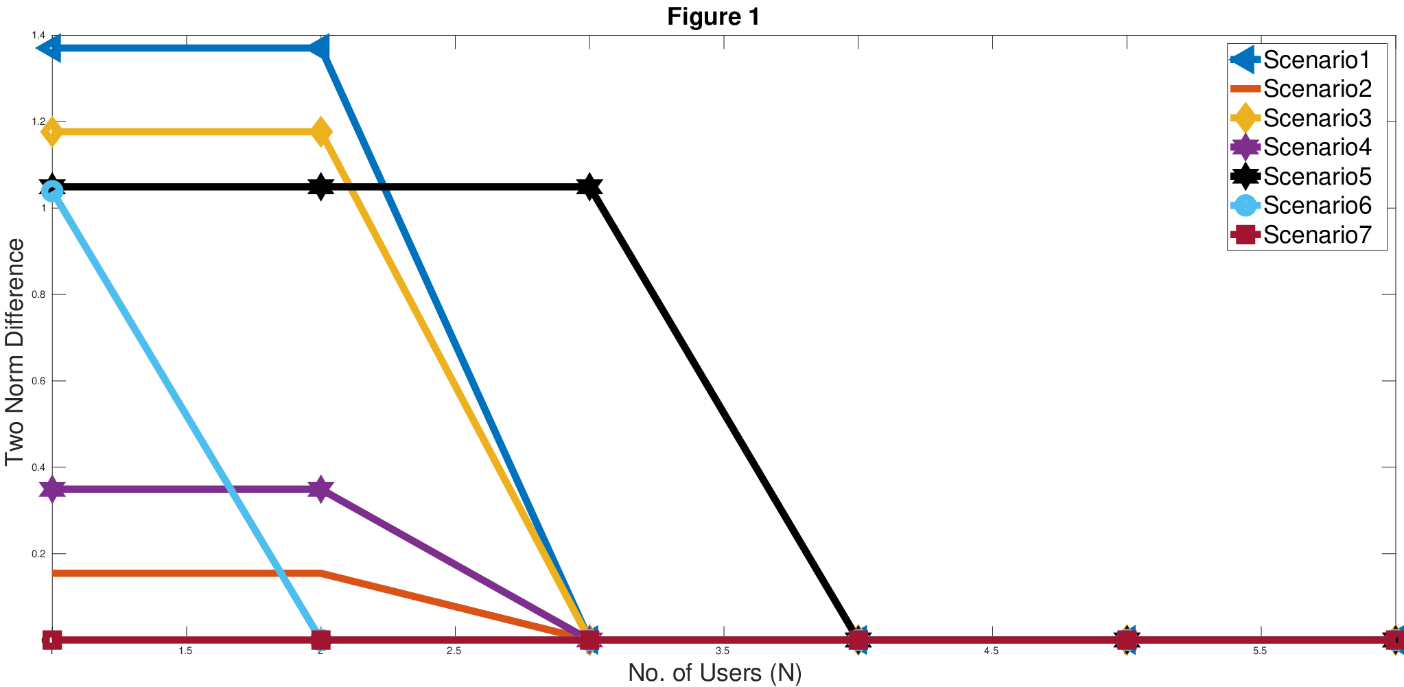
We observe from figure 1, that the NE policy of user , has become equal to the IINE policy when the number of users exceed as shown in table (I).
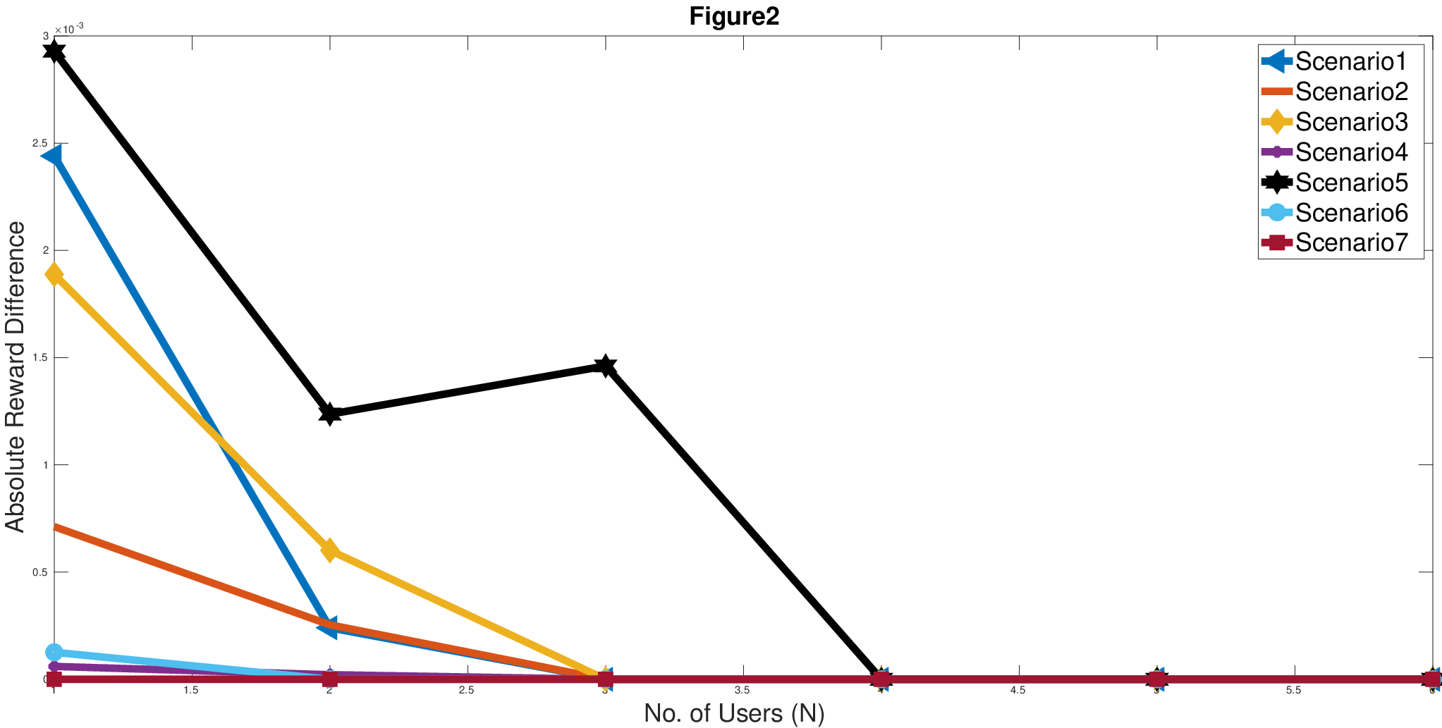
Thus after , there is no need to use the computationally expensive Iterative best response algorithm, and rather we can compute the IINE policy simply. The same result is enforced in figure 2. Here we plot the absolute difference between the time average rate of user , when all the users use their NE policies and the time average rate of user , when all the users use their IINE policies, against the number of users That is, we plot versus , where represents the NE policies of all the users, when there are players in the game and represents the IINE polices of the users. Here also we can see that after the critical number , the equilibrium reward of user is the same as the reward when all the users employ their IINE policy. Indeed as in these scenarios, the NE polices have become equal to the IINE policies as shown in figure 1, the rewards then also become the same.
From table I, is for secnario . This implies that the IINE is a NE policy when total number of users exceeds .As there have to be atleast one user, hence for this scenario, the IINE is a optimal solution to the single user problem where the user maximzies their own rate subject to power and queue constraint. Futhermore as shown in Figure 1 and Figure 2 this policy remains a NE policy for each user irrespective of number of users in the system.
In Figure 3, we plot the absolute difference of One-sensitive reawrds of user computed at the Nash equilibrium policies and the IINE policy of user versus the number of users(N). Recall that the One-sensitive reward when user employs policy is
| (19) |
This is simply the time average SNR of user at policy and from 8, the IINE maximizes the time average SNR. In Figure 3, we plot versus the number of users . As observed in Figure 3, the NE policies maximize the One-sensitive reward of user , once the number of users crosses . Indeed, as once the number of users cross the NE policies are infinitely invariant and hence maximize the time average SNR. Also in scenario , irrespective of number of users, these policies always are One-sensitive optimal, as here .

VII Conclusions
In this paper, we analyzed the scenario where multiple transmitters can send atmost one packet to a single receiver simultaneously over the multiple access channel. We model this problem as a Constrained Markov game with independent state information. That is, each user only knows his own states and actions but only knows the statistics of the state and actions of the other users. Each user selfishly maximized their own rate by choosing a power and queue allocation policy subject to power and queue constraints. We showed the existence of Nash equilibrium in this setup and provided an iterative best response algorithm to compute this equilibrium for any number of users. We showed that under the assumption of “finitely symmetric users”, there exists an infinitely invariant Nash equilibrium; that is, when the total number of users crosses a particular threshold (), the Nash equilibrium policies of each user remains the same. We then showed that an IINE can be computed by solving a finte sequence of Linear programs.
Appendix A Proof of theorem 3
Proof:
We first observe that,
The equality () in the above proof follows from reversing the steps of the above result. Equality follows from the observation that . ∎
Appendix B Proof of theorem 7
Before, we provide the proof of theorem (7), we give some definition and notation which are used repeatedly. We use Asymptotic notation, i.e, given two real valued functions, and on the set of natural numbers, denote, , and whenever there exist constants and , both strictly greater than and a natural number such that for all , , or respectively. We also denote
| (20) |
where the random variable is defined as,
| (21) |
where is an IINE policy of user . Note that, from assumptions of Theorem (7), we show in Lemma (3) and . The following well known inequality is also used heavily in our work. We mention it without proof.
Theorem 10 (Hoeffding’s Inequality ).
We have for some constant ,
| (22) |
We mention that certain Lemmas required in the proof of theorem (7) are provided after the statement of the proof.
Proof:
We first show that if , then is an IINE policy. We have from Lemma (2), that . Let denote any feasible policy of user such that it is also a vertex/endpoint of the polyhedron and . We shall prove that there exist some positive number such that for all , .
| (23) | ||||
As , there exist a positive integer such that . Let represent the smallest such integer. Then . Then using a Taylor series expansion in the previous expression (23), we have for some constant ,
| (24) |
Hence there exist a positive number such that for all , . Let denote the positive number such that for all , , where represents a vertex/endpoint of the polyhedron and . We claim that for all ,for all . Indeed, to verify (9), it suffices to consider only the vertices of the polyhedron as the optimization problem (9) is a Linear program. Clearly, we have that for , , where represents a vertex/endpoint of the polyhedron and . Now consider those points , which belong to the set and are also vertex of the polyhedron . Then we have, from (17), , for all Hence if we define the distribution
then we see that the SNR random variable has the same moments according to the distributions and Hence, by method of moments, we have It can be shown now that , for any . In particular, this implies that , for all . Hence, we have that , for all for all and , thus is a IINE policy.
We now prove the converse. Let denote an IINE policy for user , we shall prove that using induction. As is an IINE policy, we have from definition (6) and (21) that for any policy , for all
| (25) | ||||
At sufficiently large , we have using a Taylor series expansion, for some constant
Using Lemma (1), the latter is,
| (26) |
Applying the latter bound (26) to get an upper bound for (25), we have for some constants , both strictly greater than
Letting , we get that We now assume that the result is true till , i.e we show that We then have by Taylor series expansion,
| (27) |
where the last equality follows from Lemma (1). As is an IINE policy, we have from definition (6) and (21) that for any policy , for all
| (28) | ||||
Using (27) we get a upper bound for the latter (28),Hence we have for some constants , both strictly greater than
| (29) | ||||
| (30) | ||||
Letting , we get that Hence by induction, . ∎
Lemma 1.
We have, for each natural number ,
| (31) |
| (32) |
Proof:
We prove statement (31). Using , we have that ,
| (33) |
To prove the other way, we have
Proof of theorem 7
where the last inequality follows from Hoeffding’s inequality (22) . Hence,
| (34) |
and (31) follows from (33) and (34). We now prove statement (32). Using the proof technique as carried out for (31), we have,
Hence we have (32). ∎In the next lemma we show that under the assumption that the channel provides a positive reward for transmission and that there is always data to transmit , there always exists some policy such that
Lemma 2 (Feasible Policy).
Assume and . Consider the stationary policy for user ,
where . Given any value of Queue constraint and Power constraint , there exist some value of , under which both the constraints are satisfied. Also, under the same value of , we have
Proof:
Let represent the occupation measure corresponding to the stationary policy . Let , , and . It can be easily verified under the policy , the fading process and the queue process are independent. Also the queue process is ergodic with a single communicating class consisting of the whole set We denote , and as the stationary probability of being in channel state , stationary probability of queue state and the joint stationary probability of state Then , , and The transition probability of the queue process under the policy is given by,
Using the steady state equations, for the queue process, we can show that,
where Note that if and only if and hence if and only if . The average queue length under the policy is,
| (35) |
The average power expenditure under policy is,
Now by choosing , we can ensure that the average queue and power constraint will get satisfied. We now compute for the policy Define
| (36) |
As user , always transmit when his queue is not empty, we have , for all . Thus, we have in (36) ,
Thus if we ensure (or equivalently ) and , then . ∎
Lemma 3.
Let denote an IINE policy of user and let the random variable be,
| (37) |
Then
| (38) |
Proof:
As the IINE policy is a NE policy, we shall prove that for any best response policy . To do so, we first define the set of all best response of user as,
| (39) |
where denotes the the set of all policies of users other than , when the set containing the number in the game . Let denote the class of all the subsets of the set , which are obtained as convex closure of finitely many vertices of the polyhedron . As the vertices of the polyhedron is finite, we have the class itself as finite. We note that the set contains all the best response policies of user , when users other than user play multi-policy . As this set contains all the set of solutions of a linear program, we have that this set is the convex closure of finitely many points, each point being a vertex of the set of feasible occupation measures of user . This implies that the best response set belongs to the class for each multi-policy of users other than user . As the class is finite, we have that the set is a finite union of compact sets. Hence is compact. As the IINE belongs to the set , it suffices to show that . As the set is compact, we simply show that for any policy Let be any best response policy of user for some game , when the other users employ policy . Let denote any arbitrary policy of user . Then we have that if and only if . By lemma (2), we have a policy such that , hence we have,. Thus for the policy This shows that . ∎
Appendix C Proof of Theorem 8 and Theorem 9
Proof:
We note that by assumptions in Theorem (7), we have that is non-empty, hence there exist a point Hence by, statement (15), the sets are nonempty. By property (18), the set is non-empty. Thus by theorem (7), there exist an IINE. We now show that , where . Let and represent two distinct policies belonging to the set and respectively. Hence, we have that both policies belong to . We shall now show that . Let denote the SNR random variable which take values in the set . We order the set as , with , and . Define two probability distributions, and such that,
| (40) |
Let and represent the th moments of the random variable with respect to the two distributions and . As and represent two distinct policies belonging to the set , we have If we define a matrix of size with entries , then we have , where the vectors are defined as and respectively. However, as is an invertible matrix, we have and hence Now as the distributions are the same, this implies that the moments and are the same for all . As and , we have that and hence . ∎
Proof:
Let and represent two IINE policies for each user . Define two probability distributions and as in (40). We can now show by a computation that for each set
where the are SNR random variables which takes values in the set As and are both IINE policies for user , by using a similar argument as done in the proof of Theorem (8), we have that , and hence . Thus the IINE policies are interchangeable. ∎
References
- [1] Z. Han, D. Niyato, W. Saad, T. Basar, and A. Hjorungnes, Game Theory in Wireless and Communication Networks: Theory, Models, and Applications. Cambridge University Press, 2011.
- [2] L. Lai and H. E. Gamal, “The water-filling game in fading multiple-access channels,” IEEE Transaction on Information Theory, vol. 54, no. 5, pp. 2110–2122, May 2008.
- [3] G. Scutari, D. P. Palomar, and S. Barbarossa, “Optimal linear precoding strategies for wideband noncooperative systems based on game theory part 1: Nash equilibria,” IEEE Transaction on Signal Processing, vol. 56, no. 3, pp. 1230–1249, March 2008.
- [4] G. Scutari, D. P. Palomar, and S. Barbarossa, “Optimal linear precoding strategies for wideband noncooperative systems based on game theory part 2: Algorithms,” IEEE Transaction on Signal Processing, vol. 56, no. 3, pp. 1250–1267, March 2008.
- [5] D. Qiao, M. C. Gursoy, and S. Velipasalar, “A noncooperative power control game in multiple-access fading channels with qos constraints,” 2010 IEEE Wireless Communication and Networking Conference, pp. 1–6, April 2010.
- [6] T. Heikkinen, “A potential game approach to distributed power control and scheduling,” Computer Networks, vol. 50, no. 13, pp. 2295–2311, September 2006.
- [7] G. Heand, M. Debbah, and E. Altman, “A bayesian game-theoretic approach for distributed resource allocation in fading multiple access channels,” EURASIP Journal on Wireless Communications and Networking, vol. 2010, p. 391684, Apr 2010.
- [8] E. Altman, K. Avrachenkov, I. Menache, G. Miller, B. J. Prabhu, and A. Shwartz, “Dynamic discrete power control in cellular networks,” IEEE Transactions on Automatic Control, vol. 54, pp. 2328–2340, Oct 2009.
- [9] P. Narayanan and L. N. Theagarajan, “The invariant nash equilibrium for stochastic games in multiple access channel,” 2018 16th International Symposium on Modeling and Optimization in Mobile, Ad Hoc and Wireless Networks (WiOpt), pp. 1–6, May 2018.
- [10] E. Altman, K. Avratchenkov, N. Bonneau, M. Debbah, R. El-Azouzi, and D. S. Menasche, “Constrained stochastic games in wireless networks,” IEEE GLOBECOM 2007 - IEEE Global Telecommunications Conference, pp. 315–320, Nov 2007.
- [11] E. Altman, K. Avrachenkov, N. Bonneau, M. Debbah, R. El-Azouzi, and D. S. Menasche, “Constrained cost-coupled stochastic games with independent state processes,” Operations Research Letters, vol. 36, no. 2, pp. 160 – 164, 2008.
- [12] W. H. Sandholm, Population games and evolutionary dynamics. MIT press, 2010.
- [13] C. Singh, A. Kumar, and R. Sundaresan, “Uplink power control and base station association in multichannel cellular networks,” pp. 43–51, 2009.
- [14] O. Gueant, J.-M. Lasry, and P.-L. Lions, “Mean field games and applications,” Paris-Princeton lectures on mathematical finance 2010, pp. 205–266, 2011.
- [15] J.-M. Lasry and P.-L. Lions, “Mean field games,” Japanese journal of mathematics, vol. 2, no. 1, pp. 229–260, 2007.
- [16] F. Meriaux, V. Varma, and S. Lasaulce, “Mean field energy games in wireless networks,” 2012 conference record of the forty sixth Asilomar conference on signals, systems and computers (ASILOMAR), pp. 671–675, 2012.
- [17] E. Altman, Constrained Markov decision processes, vol. 7. CRC Press, 1999.
- [18] P. Narayanan and L. N. Theagarajan, “Discrete power control stochastic game on the multiple access channel,” arXiv preprint arXiv:1710.08800, 2017.