Supervisor Localization of Discrete-Event Systems with Infinite Behavior
(August 24, 2026)

Renyuan Zhang Affiliation: R. Zhang is with School of Automation, Northwestern Polytechnical University, China. Email: ryzhang@nwpu.edu.cn. Kai Cai Affiliation: K. Cai is with Department of Electrical and Information Engineering, Osaka City University, Japan. Email: kai.cai@eng.osaka-cu.ac.jp.

Abstract

Recently we developed supervisor localization, a top-down approach to distributed control of discrete-event systems (DES) with finite behavior. Its essence is the allocation of monolithic (global) control action among the local control strategies of individual agents. In this report, we extend supervisor localization to study the distributed control of DES with infinite behavior. Specifically, we first employ Thistle and Wonham’s supervisory control theory for DES with infinite behavior to compute a safety supervisor (for safety specifications) and a liveness supervisor (for liveness specifications), and then design a suitable localization procedure to decompose the safety supervisor into a set of safety local controllers, one for each controllable event, and decompose the liveness supervisor into a set of liveness local controllers, two for each controllable event. The localization procedure for decomposing the liveness supervisor is novel; in particular, a local controller is responsible for disabling the corresponding controllable event on only part of the states of the liveness supervisor, and consequently, the derived local controller in general has states number no more than that computed by considering the disablement on all the states. Moreover, we prove that the derived local controllers achieve the same controlled behavior with the safety and liveness supervisors. We finally illustrate the result by a Small Factory example.

Index Terms:

Discrete-Event Systems, Supervisory Control, Infinite Behavior, Supervisor Localization

I Introduction

In [1, 2, 3, 4, 5, 6] we developed a top-down approach, called supervisor localization, to the distributed control of multi-agent discrete-event systems (DES). This approach first synthesizes a monolithic supervisor (or a heterarchical array of modular supervisors), and then decomposes the supervisor into a set of local controllers for the component agents. Localization creates a purely distributed control architecture in which each agent is controlled by its own local controller; this is particularly suitable for applications consisting of many autonomous components, e.g. multi-robot systems. Moreover, localization can significantly improve the comprehensibility of control logic, because the resulting local controllers typically have many fewer states than their parent supervisor.

These works focus on DES with finite behaviors [7], in which DES are modelled as generators accepting $*$ -languages (consisting of finite-length strings) and the specifications are expressed by $*$ -languages. In modelling and control of reactive systems (e.g. automated factories, operating systems, communication protocols), however, the systems may operate indefinitely, and the specifications may require that every system component must operate infinitely often. In these cases, $\omega$ -automata on infinite inputs and $\omega$ -languages consisting of infinite-length strings were introduced to model the DES with infinite behavior and specify the specifications respectively. Notable works on synthesizing supervisors for the DES with infinite behavior include the following. First, Ramadge [8] models the DES with infinite behavior by Büchi automata and derives conditions ( $*$ -controllability and $\omega$ -closure) for the existences of supervisors; within the same framework, Young et al. [9] derives another supervisor existence condition (replacing $\omega$ -closure by finite stabilizability) under less restrictive conditions. Then, Thistle and Wonham [10, 11, 12] introduce the concept of $\omega$ -controllability which is closed under arbitrary set union, and develop a procedure to synthesize supervisors satisfying given specifications expressed by $\omega$ -languages; Kumar et al. [13] proposed an alternative algorithm to compute the supremal $\omega$ -controllable sublanguage. Later, Thistle [14] extend the result in [10] to a more general case where the plant DES are modelled by deterministic Rabin-automata. More recently, Thistle and Lamouchi [15] addressed the issue of partial observation in the supervisory control of DES with infinite behavior. To the best of our knowledge, however, there is no result on distributed control for multi-agent DES with infinite behavior reported in the literature.

In this paper, we extend supervisor localization to address distributed control for DES with infinite behavior. Our approach is as follows. Given a DES plant with infinite behavior and safety and liveness specifications, we first synthesize a safety supervisor (for safety specifications) and a liveness supervisor (for liveness specifications) by the method proposed by Thistle and Wonham [10, 12]. The infinite controlled behavior of the plant is restricted through the control actions on finite strings, thus as in DES with finite behavior [7], we implement the supervisors by $*$ -automata. We then adopt the localization procedure in [1] with suitable modifications to decompose the automata-based safety and liveness supervisors into local controllers for individual controllable events. Moreover we prove that the derived local controllers are control equivalent to the synthesized safety and liveness supervisors.

The contributions of this paper are twofold. First, we develop a new supervisor localization theory for DES with infinite behavior in Thistle and Wonham’s supervisory control framework [12], which supplies a systematic, computationally effective approach to distributed control of multi-agent DES with infinite behavior. In particular, we first decompose the safety supervisor into a set of local controllers, one for each controllable event, by the localization procedure in [1]; then we decompose the liveness supervisor into a set of local controllers, however, two for each controllable events, by a newly developed localization procedure. The central idea of the new procedure is the new definition of disabling function with a new language: only the disablement on part of the states are defined, i.e. an event is defined as disabled at one state only if the state can be visited by strings in the given language. With this new disabling function, we define new concepts of control consistency and control cover, and the resultant local controllers in general have states number no more than that computed by the localization procedure in [1] where the disablement on all the states are considered.

Second, we identify the essence of localization procedure for DES with infinite behavior: only the disabling/enabling actions on finite strings need be considered. Namely, if the control equivalence of the local controllers with their parent supervisors on finite behavior is guaranteed, the control equivalence on infinite behavior can be derived by Lemma 1 in Section IV-C, which declares that the operator limit (mapping finite strings to infinite strings whose prefixes are all contained in the given finite strings) will not change the language equivalence on intersections. Consequently, control consistency relation and control cover, the central concepts of the localization procedure, are defined only on the disabling and enabling functions, irrelevant to the infinite behaviors. We demonstrate the above result by a case study of Small Factory example [10].

Our proposed localization procedure can in principle be used to construct local controllers from supervisors computed by any other synthesis method for DES with infinite behavior e.g. [8, 9, 14]. In this paper, we adopt the Thistle and Wonham’s supervisory control theory for two reasons. First, it extends basic results of the supervisory control theory of Ramadge and Wonham [16, 7] for DES with finite behavior to infinite behavior, and generalizes results of [8] to the case in which specification languages need not be $\omega$ -closed relative to plant behavior. Second, the supervisors synthesized by Thistle and Wonham’s theory can be implemented by $*$ -automata, which are eligible to be decomposed into local controllers by our previous work on supervisor localization procedure with appropriate modifications.

The paper is organized as follows. Section II reviews the preliminaries on DES with infinite behavior and Thistle and Wonham’s supervisory control theory. Section III formulates the problem of Supervisor Localization for DES with infinite behavior. Section IV presents the localization procedure and proves the control equivalence of the derived local controllers with their parent supervisors, and Section V illustrates the proposed localization procedure by a Small Factory example. Finally Section VI states our conclusions.

II Preliminaries on DES with Infinite Behavior

In this section, we briefly review Thistle and Wonham’s supervisory control framework of discrete-event systems (DES) with infinite behavior [11, 12, 10].

II-A Discrete-Event Systems with Infinite Behavior

A discrete-event system (DES) with infinite behavior (plant to be controlled) is modeled as a deterministic Büchi automaton¹¹ 1 The DES with infinite behavior can also be modeled by other form of $\omega$ -automata with different types of acceptance criteria, e.g. Muller automata, Rabin automata, Street automata. It is known [17] that deterministic Büchi automata represent a strict subset of $\omega$ -regular languages, having less expressive power than nondeterministic Büchi automata, deterministic and nondeterministic Muller automata, and deterministic and nondeterministic Rabin automata which represent the full set of $\omega$ -regular languages. In this report, following Thistle and Wonham’s framework [18], we focus on the subset of $\omega$ -regular languages that are represented by deterministic Büchi automata, and leave the extension to the full set for future work.

\displaystyle{\bf G}:=(Q,\Sigma,\delta,q_{0},\mathcal{B}_{Q}),

(1)

where $Q$ is the finite state set, $q_{0}$ is the initial state, $\Sigma$ is the finite event set (alphabet), $\delta:Q\times\Sigma\rightarrow Q$ is the (partial) state transition function, and $\mathcal{B}_{Q}\subseteq Q$ is the Büchi acceptance criterion. In the usual way, $\delta$ is extended to $\delta:Q\times\Sigma^{*}\rightarrow Q$ , and we write $\delta(q,s)!$ to mean that $\delta(q,s)$ is defined. Let $\Sigma^{*}$ be the set of all finite strings over $\Sigma$ , including the empty string $\epsilon$ , and $\Sigma^{\omega}$ the set of all infinite strings over $\Sigma$ ; the disjoint union of $\Sigma^{*}$ and $\Sigma^{\omega}$ is denoted by $\Sigma^{\infty}$ , i.e. $\Sigma^{\infty}=\Sigma^{*}\dot{\cup}\Sigma^{\omega}$ . The DES ${\bf G}$ has both finite behavior and infinite behavior. The finite behavior of ${\bf G}$ is the $*$ -language $L({\bf G})\subseteq\Sigma^{*}$ accepted by the $*$ -automaton $(Q,\Sigma,\delta,q_{0})$ , i.e.

L({\bf G}):=\{s\in\Sigma^{*}|\delta(q,s)!~\&~\delta(q,s)\in Q\};

and the infinite behavior of ${\bf G}$ is the $\omega$ -language $S({\bf G})$ accepted by the $\omega$ -automaton ${\bf G}$ with Büchi acceptance criterion $\mathcal{B}_{Q}$ , i.e.

S({\bf G}):=\{s\in\Sigma^{\omega}|\Omega(s)\cap\mathcal{B}_{Q}\neq\emptyset\}

where $\Omega(s)$ is set of states that $s$ visits infinitely often.

A string $s\in\Sigma^{*}$ is a prefix of a string $v\in\Sigma^{\infty}$ , written $s\leq v$ , if there exists $t\in\Sigma^{\infty}$ such that $v=st$ . The (prefix) $*$ -closure of a language $K\subseteq\Sigma^{\infty}$ is defined by

\displaystyle pre(K):=\{s\in\Sigma^{*}|(\exists s_{1}\in K)~s\leq s_{1}\}

(2)

If $K=pre(K)$ , we say that $K$ is $*$ -closed. In this report, we assume that (i) $pre(L({\bf G}))=L({\bf G})$ , i.e. $L(\bf G)$ is $*$ -closed, and (ii) $pre(S({\bf G}))=L({\bf G})$ , i.e. ${\bf G}$ is deadlock-free. Define the limit of a $*$ -language $K$ by

\displaystyle lim(K):=pre^{-1}(K)\cap\Sigma^{\omega}

(3)

where $pre^{-1}(K):=\{v\in\Sigma^{\infty}|pre(v)\subseteq K\}$ ; then the $\omega$ -closure of an $\omega$ -language $R$ is given by

\displaystyle clo(R):=lim(pre(R))=pre^{-1}(pre(R))\cap\Sigma^{\omega}.

(4)

If $R=clo(R)$ , we say that $R$ is $\omega$ -closed; if $R=clo(R)\cap S$ , we say that $R$ is $\omega$ -closed with respect to $S$ . Note that $S(\bf G)$ represents a liveness assumption in the modelling of ${\bf G}$ , and in general $S({\bf G})\subseteq lim(L({\bf G}))$ ; so $S(\bf G)$ itself need not be $\omega$ -closed.

II-B Supervisory Control for DES with Infinite Behavior

For supervisory control, the event set $\Sigma$ is partitioned into $\Sigma_{c}$ , the subset of controllable events that can be disabled by an external supervisor, and $\Sigma_{uc}$ , is the subset of uncontrollable events that cannot be prevented from occurring (i.e. $\Sigma=\Sigma_{c}~\dot{\cup}~\Sigma_{uc}$ ). A supervisory control for $\bf G$ is any map $f:L({\bf G})\rightarrow\Gamma$ , where $\Gamma:=\{\gamma\subseteq\Sigma|\gamma\supseteq\Sigma_{u}\}$ . Then the finite and infinite closed-loop behaviors of the controlled DES ${\bf G}^{f}$ , representing the action of the supervisor $f$ on $\bf G$ , are respectively given by

(a)

$L({\bf G}^{f})$ , the $*$ -language synthesized by $f$ , is defined by the following recursion:

	(i)	$\displaystyle\epsilon\in L({\bf G}^{f}),$
	(ii)	$\displaystyle(\forall s\in\Sigma^{*},\sigma\in\Sigma)~s\sigma\in L({\bf G}^{f})\Leftrightarrow s\in L({\bf G}^{f})~\&~$
		$\displaystyle s\sigma\in L({\bf G})~\&~\sigma\in f(s);$

(b)

$S({\bf G}^{f})$ , the $w$ -language synthesized by $f$ , is given by

$\displaystyle S({\bf G}^{f}):=lim(L({\bf G}^{f}))\cap S({\bf G})$ (5)

The definition of $L({\bf G}^{f})$ means that a string $s\sigma$ can occur under supervision if and only if the string $s$ can occur under supervision, and the event $\sigma$ can take place without violating either the ‘physical’ constraints embodied by $L({\bf G})$ or the control pattern imposed by the supervisor. The definition of $S({\bf G}^{f})$ says that an infinite string $s\in S({\bf G})$ can eventually occur if and only if it can occur in the absence of supervision and the supervisor does not prevent the occurrence of any of its its prefixes in $pre(s)$ . Namely, $f$ exert its influence on infinite strings only through the control actions on their finite prefixes. We say that $f:L(\bf G)\rightarrow\Gamma$ is a complete supervisor for $\bf G$ if $L({\bf G}^{f})\subseteq L({\bf G})$ , and a deadlock-free supervisor if ${\bf G}^{f}$ is a deadlock-free DES, i.e. $pre(S({\bf G}^{f}))=L({\bf G}^{f})$ .

There are two classes of control requirements imposed on $\bf G$ : safety specifications describing that some conditions on $\bf G$ will not occur, and liveness specifications requiring that some other conditions must occur eventually [19]. The safety and liveness specifications can be specified in terms of $*$ -languages and $\omega$ -languages, respectively. In the following we briefly introduce the supervisory control for $\bf G$ with infinite behavior.

First, for safety specifications, consider supervisory control of the finite behavior of $\bf G$ ; it is proved [20] that there exists a complete supervisor $f^{*}:L({\bf G})\rightarrow\Gamma$ that synthesizes a $*$ -language $K\subseteq L({\bf G})$ if and only if $K$ is $*$ -controllable with respect to $\bf G$ and $*$ -closed with respect to $L(\bf G)$ .

Formally, language $K\subseteq\Sigma^{\infty}$ is $*$ -controllable with respect to $\bf G$ (or $L({\bf G})$ ) if

\displaystyle pre(K)\Sigma_{u}\cap pre(L({\bf G}))\subseteq pre(K).

Let $*$ -language $E_{s}$ represent a safety specification imposed on $\bf G$ , and

	$\displaystyle\mathcal{C}^{*}(E_{s}):=\{K\subseteq L({\bf G})\|~$	$\displaystyle K\subseteq E_{s}~\text{and}$
		$K$ is $*$ -controllable wrt. ${\bf G}$ and
		$\displaystyle\text{$*$-closed wrt.}~L({\bf G})\}$

the set of $*$ -controllable and $*$ -closed sublanguages of $E_{s}$ . Since $*$ -controllability and $*$ -closure are both closed under arbitrary set union, there exists the supremal $*$ -controllable and $*$ -closed sublanguage $\sup\mathcal{C}^{*}(E_{s})$ which may be effectively computed, and furthermore, a complete and deadlock-free supervisor

\displaystyle f^{*}:L({\bf G})\rightarrow\Gamma

(6)

synthesizing $\sup\mathcal{C}^{*}(E_{s})$ , i.e.

\displaystyle L({\bf G}^{f^{*}})

\displaystyle=\sup\mathcal{C}^{*}(E_{s})

can be constructed [7, 20].

Then for liveness specifications, consider supervisory control of infinite behavior of $\bf G$ ; it is proved [12, Proposition 4.5] that there exists a complete and deadlock-free supervisor $f^{\omega}:L({\bf G})\rightarrow\Gamma$ that synthesizes an $\omega$ -language $T\subseteq S({\bf G})$ if and only if $T$ is $\omega$ -controllable with respect to $\bf G$ and $\omega$ -closed with respect to $S(\bf G)$ . To introduce $\omega$ -controllability, we need the concept of controllability prefix.

For an $\omega$ -language $T\subseteq\Sigma^{\omega}$ , its controllability prefix is given by

	$\displaystyle pre_{\bf G}(T):=\{t\in pre(T)\|(\exists T^{\prime}\subseteq T/t)~[T^{\prime}\neq\emptyset~\text{is}$
	$\displaystyle*\text{-controllable wrt.}~$	$\displaystyle L({\bf G})/t~$
	$\displaystyle\text{and}~\omega\text{-closed wrt.}~$	$\displaystyle S({\bf G})/t~]\}$

where $T/t:=\{s\in\Sigma^{\infty}|ts\in T\}$ , and $L({\bf G})/t$ and $S({\bf G})/t$ are defined similarly.

Now, we define that $T$ is $\omega$ -controllable with respect to $\bf G$ if

	$\displaystyle(\textnormal{i})~$	$T$ is $*$ -controllable with respect to $\bf G$ ;
	$\displaystyle(\textnormal{ii})~$	$pre(T)=pre_{\bf G}(T)$ .

Note that $\omega$ -controllable and $\omega$ -closed languages have different closure properties under union and intersection. Specifically, $\omega$ -controllability is preserved under arbitrary unions but not intersections, while $\omega$ -closure is preserved under arbitrary intersections but not unions. It is therefore convenient to define, below, the separate language classes:

	$\displaystyle\mathcal{C}^{\omega}(E_{l}):=\{T\subseteq S({\bf G})\|~$	$\displaystyle T\subseteq E_{l}~\text{and}$
		$\displaystyle\text{$T$ is $\omega$-controllable wrt.}~{\bf G}\}$
	$\displaystyle\mathcal{F}^{\omega}(A):=\{T\subseteq S({\bf G})\|~$	$\displaystyle A\subseteq T~\text{and}$
		$\displaystyle\text{$T$ is $\omega$-closed wrt.}~S({\bf G})\}$

where $E_{l}$ is an $\omega$ -language representing the maximal legal specification and $A$ is also an $\omega$ -language but representing the minimal acceptable specification. Due to the closure property of $\omega$ -controllability and $\omega$ -closure described above, there exists [12, Proposition 5.2] the unique supremal $\omega$ -controllable sublanguage $\sup\mathcal{C}^{\omega}(E_{l})$ , given by

\displaystyle\sup\mathcal{C}^{\omega}(E_{l}):=lim(pre_{\bf G}(E_{l}))\cap E_{l}

and the unique infimal $\omega$ -closed superlanguage $\inf\mathcal{F}^{\omega}(A)$ , given by

\displaystyle\inf\mathcal{F}^{\omega}(A):=clo(A)\cap S({\bf G}).

Furthermore, it is proved [12, Theorem 5.3] that there exists a $\omega$ -controllable and $\omega$ -closed language $T$ such that $A\subset T\subseteq E_{l}$ if and only if

\displaystyle\inf\mathcal{F}^{\omega}(A)\subseteq\sup\mathcal{C}^{\omega}(E_{l})

(7)

and if exists, a complete and deadlock-free supervisor

\displaystyle f^{\omega}:L({\bf G})\rightarrow\Gamma

(8)

synthesizing such $T$ , i.e.

	$\displaystyle A\subset T=S({\bf G}^{f^{\omega}})\subseteq E_{l}$		(9)
	$\displaystyle pre(S({\bf G}^{f^{\omega}}))=L({\bf G}^{f^{\omega}})$		(10)

can be constructed according to the procedure described in Appendix A.

III Problem Formulation

Let $\bf G$ as in (1) be the plant to be controlled, $E_{s}$ the safety specification, $E_{l}$ the maximal legal liveness specification, and $A$ the minimal acceptable liveness specification. To synthesize supervisors for these specifications, our approach is in a simple but natural way: first synthesize a supervisor $f^{*}$ for the safety specification; then treat the closed-loop behavior of $\bf G$ controlled by $f^{*}$ as the new plant to be controlled, and synthesize another supervisor $f^{\omega}$ for the liveness specifications. By this approach, the supervisors $f^{*}$ and $f^{\omega}$ work conjunctively, without conflicts, because the controlled behavior of $f^{*}$ is the plant behavior of $f^{\omega}$ and thus a controllable event that has been disabled by $f^{*}$ need not be disabled by $f^{\omega}$ again.

First, for the safety specification $E_{s}$ , we synthesize as in (6) a complete supervisor $f^{*}:L({\bf G})\rightarrow\Gamma$ such that the finite behavior of $\bf G$ under the control of $f^{*}$ , denoted by ${\bf G}^{f^{*}}$ , satisfies

\displaystyle L({\bf G}^{f^{*}})

\displaystyle=\sup\mathcal{C}^{*}(E_{s}).

According to (5), the infinite controlled behavior of ${\bf G}$ is $S({\bf G}^{f^{*}})=S({\bf G})\cap lim(L({\bf G}^{f^{*}}))$ ; ${\bf G}^{f^{*}}$ can be represented by a deterministic Büchi automaton $(X^{*},\Sigma,\xi^{*},x_{0}^{*},\mathcal{B}_{X^{*}})$ constructed according to

(i)

Select $x_{0}^{*}\in X^{*}$ corresponding to $q_{0}\in Q$ .
(ii)

$\xi^{*}:X^{*}\times\Sigma\rightarrow X^{*}$ with $\xi^{*}(x^{*},\sigma)=x^{\prime*}$ if there exists $s\in\Sigma^{*}$ such that $\xi^{*}(x_{0}^{*},s)=x^{*}$ , $\delta(q_{0},s\sigma)!$ , and $\sigma\in f^{*}(s)$ .
(iii)

$\mathcal{B}_{X^{*}}:=\{x^{*}\in X^{*}|(\exists s\in\Sigma^{*})~\xi^{*}(x_{0}^{*},s)=x^{*},\delta(q_{0},s)\in\mathcal{B}_{Q}\}$ .

Let

\displaystyle{\bf SUP}^{*}:=(X^{*},\Sigma,\xi^{*},x_{0}^{*}).

(11)

Namely ${\bf SUP}^{*}$ has the same transition structure and thus same finite behavior as ${\bf G}^{f^{*}}$ , i.e. $L({\bf SUP}^{*})=L({\bf G}^{f^{*}})$ . Then ${\bf SUP}^{*}$ is an implementation [7] of the supervisor $f^{*}$ , i.e.

\displaystyle L({\bf G})\cap L({\bf SUP}^{*})

\displaystyle=L({\bf G}^{f^{*}})

Since $L({\bf SUP}^{*})=L({\bf G}^{f^{*}})$ , it also infers that $S({\bf G}^{f^{*}})=S({\bf G})\cap lim(L({\bf SUP}^{*}))$ .

Second, we consider the supervisor synthesis for the liveness specifications $E_{l}$ and $A$ . At this step, we treat ${\bf G}^{f^{*}}$ as the new plant to be controlled, and synthesize as in (8) a complete and deadlock-free supervisor $f^{\omega}:L({\bf G}^{f^{*}})\rightarrow\Gamma$ given by

f^{\omega}(l):=\left\{\begin{array}[]{ll}f_{0}^{\omega}(l)&\text{if}~l\in pre(A),\\ f_{k}^{\omega}(l/k)&\text{if}~l\in k~pre(E_{k}^{\prime}),k\in M\\ \text{undefined}&\text{otherwise}\end{array}\right.

(12)

where $M$ is the set of all elements of $pre(\sup\mathcal{C}^{\omega}(E_{l}))\setminus pre(\inf\mathcal{F}^{\omega}(A))$ of minimal length, and $E_{k}^{\prime}$ is the sublanguage of $\sup\mathcal{C}^{\omega}(E_{l})/k$ synthesized by $f_{k}^{\omega}$ . Under the supervision of $f^{\omega}$ , the infinite controlled behavior of ${\bf G}^{f^{*}}$ , denoted by ${\bf G}^{f^{*}\wedge f^{\omega}}$ ( $f^{*}$ and $f^{\omega}$ work conjunctively, i.e. a controllable event will be disabled if it is disabled by any one of $f^{*}$ and $f^{\omega}$ ), satisfies:

		$\displaystyle A\subseteq S({\bf G}^{f^{*}\wedge f^{\omega}})\subseteq E_{l}$
		$\displaystyle pre(S({\bf G}^{f^{}\wedge f^{\omega}}))=L({\bf G}^{f^{}\wedge f^{\omega}}).$

${\bf G}^{f^{*}\wedge f^{\omega}}$ can be represented by a deterministic Büchi automaton $(X^{\omega},\Sigma,\xi^{\omega},x_{0}^{\omega},\mathcal{B}_{X^{\omega}})$ constructed by:

(i)

Select $x_{0}^{\omega}\in X^{\omega}$ corresponds to $x_{0}^{*}\in X^{*}$ .
(ii)

$\xi^{\omega}:X^{\omega}\times\Sigma\rightarrow X^{\omega}$ with $\xi^{\omega}(x^{\omega},\sigma)={x^{\prime}}^{\omega}$ if there exists $s\in\Sigma^{*}$ such that $\xi^{\omega}(x_{0}^{\omega},s)=x^{\omega}$ , $\xi^{*}(x_{0}^{*},s\sigma)!$ , and $\sigma\in f^{\omega}(s)$ .
(iii)

$\mathcal{B}_{X^{\omega}}:=\{x^{\omega}\in X^{\omega}|(\exists s\in\Sigma^{*})~\xi^{\omega}(x_{0}^{\omega},s)=x^{\omega},\xi(x_{0}^{*},s)\in\mathcal{B}_{X^{*}}\}$ .

The supervisor $f^{\omega}:\Sigma^{*}\rightarrow\Gamma$ exercises its control action depending on its observation on finite strings in $\Sigma^{*}$ , and thus $f^{\omega}$ also can be implemented by a *-automaton. Let

\displaystyle{\bf SUP}^{\omega}:=(X^{\omega},\Sigma,\xi^{\omega},x_{0}^{\omega}).

(13)

Namely ${\bf SUP}^{\omega}$ has the same transition structure and thus same finite behavior as ${\bf G}^{f^{*}\wedge f^{\omega}}$ , i.e. $L({\bf SUP}^{\omega})=L({\bf G}^{f^{*}\wedge f^{\omega}})$ . Then ${\bf SUP}^{\omega}$ is an implementation of the supervisor $f^{\omega}$ , i.e.

\displaystyle S({\bf G}^{f^{*}})\cap lim(L({\bf SUP}^{\omega}))

\displaystyle=S({\bf G}^{f^{*}\wedge f^{\omega}}).

(14)

Note that ${\bf SUP}^{\omega}$ also influences the finite controlled behavior of $\bf G$ , thus $L({\bf G}^{f^{*}\wedge f^{\omega}})$ and $S({\bf G}^{f^{*}\wedge f^{\omega}})$ represent respectively the finite and infinite controlled behavior of $\bf G$ under the control of ${\bf SUP}^{*}$ and ${\bf SUP}^{\omega}$ , i.e.

		$\displaystyle L({\bf G}^{f^{}\wedge f^{\omega}})=L({\bf G})\cap L({\bf SUP}^{})\cap L({\bf SUP}^{\omega})$		(15)
		$\displaystyle S({\bf G}^{f^{}\wedge f^{\omega}})=S({\bf G})\cap lim(L({\bf SUP}^{}))\cap lim(L({\bf SUP}^{\omega})).$		(16)

It is easily verified that the finite controlled behavior of ${\bf G}$ satisfies the safety specification, i.e.

L({\bf G}^{f^{*}\wedge f^{\omega}})\subseteq E_{s},

and the infinite controlled behavior fits into the range of liveness specifications $E_{l}$ and $A$ , i.e.

A\subseteq S({\bf G}^{f^{*}\wedge f^{\omega}})\subseteq E_{l}.

The supervisor ${\bf SUP}^{*}$ is constructed for satisfying the safety specification and thus we refer it as the safety supervisor for $\bf G$ ; while ${\bf SUP}^{\omega}$ is constructed for the liveness specifications and thus we refer it as the liveness supervisor for $\bf G$ . Throughout this paper, we assume that $S({\bf G}^{f^{*}\wedge f^{\omega}})\neq\emptyset$ and thus $L({\bf G}^{f^{*}\wedge f^{\omega}})\neq\emptyset$ .

The control action of ${\bf SUP}^{*}$ and ${\bf SUP}^{\omega}$ are both to enable/disable controllable events; thus the localizations of ${\bf SUP}^{*}$ and ${\bf SUP}^{\omega}$ are similar to that of the monolithic supervisor $\bf SUP$ in [1]. The differences are illustrated in Fig. 1. First, the localization of $\bf SUP$ generate one local controller for each controllable event. However, the present localization procedure may generate multiple local controllers for one controllable event, because an event may be disabled/enabled by both ${\bf SUP}^{*}$ and ${\bf SUP}^{\omega}$ . Second, the localization of ${\bf SUP}^{*}$ is similar to that of $\bf SUP$ in [1], however, the localization of ${\bf SUP}^{\omega}$ is particular: according to whether or not $s\in pre(A)$ (see (12) for the definition of $f^{\omega}$ ), there are two types of supervisors included in $f^{\omega}$ : $f_{0}^{\omega}$ defined on the strings $s\in pre(A)$ and $f_{k}^{\omega}$ defined on the rest of the strings in $L({\bf G})$ , thus the localization of ${\bf SUP}^{\omega}$ can be divided into two parts and consequently, we will get two local controllers for each controllable event.

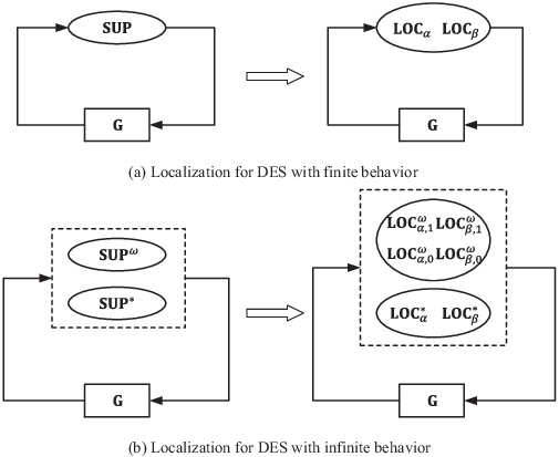
Refer to caption — Fig. 1: Supervisor localization example for illustration: let $\Sigma_{c}=\{\alpha,\beta\}$ . For DES $\bf G$ with finite behavior as in (a), the monolithic supervisor $\bf SUP$ is decomposed into two local controllers ${\bf LOC}_{\alpha}$ and ${\bf LOC}_{\beta}$ for controllable events $\alpha$ and $\beta$ respectively. For DES $\bf G$ with infinite behavior as in (b), there are two supervisors ${\bf SUP}^{*}$ and ${\bf SUP}^{\omega}$ constructed for satisfying safety specification and liveness specifications respectively. The localization procedure decomposes ${\bf SUP}^{*}$ into two local controllers ${\bf LOC}_{\alpha}^{*}$ and ${\bf LOC}_{\beta}^{*}$ , and decomposes ${\bf SUP}^{\omega}$ into local controllers ${\bf LOC}_{\alpha,0}^{*}$ and ${\bf LOC}_{\alpha,1}^{*}$ for $\alpha$ , and ${\bf LOC}_{\beta,0}^{\omega}$ and ${\bf LOC}_{\beta,1}^{\omega}$ for $\beta$ .

Remark 1.

We remark here that the localization of the control actions after string $s\notin pre(A)$ is treated as a whole, but not divided corresponding to each $f_{k}^{\omega}$ ( $k\in M$ ). The reason is as follows. First, to localize the control actions after each string $k$ , we need to find in $L({\bf SUP}^{\omega})$ the language $E_{k}^{\prime}$ synthesized by $f_{k}^{\omega}$ , which will increase the time complexity of the overall algorithm. Second, the number of local controllers will increase with the states number of ${\bf SUP}^{\omega}$ . In our current setting, all the controlled behavior synthesized by $f_{k}^{\omega}$ are contained in $L({\bf SUP}^{\omega})$ , thus we don’t have to find each $E_{k}^{\prime}$ ; consequently for each controllable event, ${\bf SUP}^{\omega}$ will be constantly decomposed into two local controllers: one corresponding to $f_{0}^{\omega}$ and the other to all $f_{k}^{\omega}$ .

Remark 2.

Note that it is also possible to construct a monolithic supervisor $\bf SUP$ that synthesizes the controlled behavior $L({\bf G}^{f^{*}\wedge f^{\omega}})$ , i.e. $\bf SUP$ is control equivalent to ${\bf SUP}^{*}$ and ${\bf SUP}^{\omega}$ . In that case, by applying the localization procedure in [1], we may get for each controllable event a local controller. In general, this local controller will have more states than the local controllers constructed by our new localization procedures, as will be demonstrated in the example of Small Factory in Section V. The reason is that either ${\bf SUP}^{*}$ , or ${\bf SUP}^{\omega}$ , disables controllable events on part of the strings in $L({\bf G})$ : the plant of ${\bf SUP}^{*}$ is $\bf G$ and the plant of ${\bf SUP}^{\omega}$ is ${\bf G}^{f^{*}}$ .

Due to the above features specific to ${\bf SUP}^{*}$ and ${\bf SUP}^{\omega}$ , we have different types of local controllers for each controllable event $\alpha\in\Sigma_{c}$ . First, we say that a *-automaton

{\bf LOC}_{\alpha}^{*}=(Y_{\alpha}^{*},\Sigma,\eta_{\alpha}^{*},y_{0,\alpha}^{*})

is a safety local controller for $\alpha$ if ${\bf LOC}_{\alpha}^{*}$ enables/disables event $\alpha$ (and only $\alpha$ ) consistently with ${\bf SUP}^{*}$ , which means that for all $s\in\Sigma^{*}$ there holds

	$\displaystyle s\alpha\in L({{\bf LOC}_{\alpha}^{}}),\ s\alpha\in L({\bf G}),~s\in L({\bf SUP}^{})$
	$\displaystyle\Leftrightarrow~s\alpha\in L({\bf SUP}^{*})$		(17)

Second, for all the strings $s\in L({\bf G}^{f^{*}})$ , we divide them into two parts: $C_{1}=pre(A)$ and $C_{2}=L({\bf G}^{f^{*}})\setminus pre(A)$ . For each part $C_{n}$ ( $n=1,2$ ), we say that a *-automaton

{\bf LOC}_{\alpha,n}^{\omega}=(Y_{\alpha,n}^{\omega},\Sigma,\eta_{\alpha,n}^{\omega},y_{0,\alpha,n}^{\omega}),

is a liveness local controller for $\alpha$ if ${\bf LOC}_{\alpha,n}^{\omega}$ enables/disables event $\alpha$ (and only $\alpha$ ) occurred at string $s\in C_{n}$ consistently with ${\bf SUP}^{\omega}$ , which means that for all $s\in C_{n}$ there holds

	$\displaystyle s\alpha\in L({{\bf LOC}_{\alpha,n}^{}}),\ s\alpha\in L({\bf G}^{f^{}}),~s\in L({\bf SUP}^{\omega})$
	$\displaystyle\Leftrightarrow~s\alpha\in L({\bf SUP}^{\omega})$		(18)

We now formulate the Supervisor Localization Problem for DES with infinite behavior:

Construct a set of safety local controllers $\{{\bf LOC}_{\alpha}^{*}\ |\ \alpha\in\Sigma_{c}\}$ , a set of liveness local controllers $\{{\bf LOC}_{\alpha,n}^{\omega}\ |\ \alpha\in\Sigma_{c},n=1,2\}$ such that their collective controlled behaviors are equivalent to those of supervisors ${\bf SUP}^{*}$ and ${\bf SUP}^{\omega}$ with respect to ${\bf G}$ , i.e.

	$\displaystyle{\scriptsize}L({\bf G})$	$\displaystyle\cap\Big(\mathop{\bigcap}\limits_{\alpha\in\Sigma_{c}}L({\bf LOC}_{\alpha}^{*})\Big)$
		$\displaystyle\cap\Big(\mathop{\bigcap}\limits_{\alpha\in\Sigma_{c},n=1,2}L({\bf LOC}_{\alpha,n}^{\omega})\Big)=~L({\bf G}^{f^{*}\wedge f^{\omega}})$
	$\displaystyle S({\bf G})$	$\displaystyle\cap\Big(\mathop{\bigcap}\limits_{\alpha\in\Sigma_{c}}lim(L({\bf LOC}_{\alpha}^{*}))\Big)$
		$\displaystyle\cap\Big(\mathop{\bigcap}\limits_{\alpha\in\Sigma_{c},n=1,2}lim(L({\bf LOC}_{\alpha,n}^{\omega}))\Big)=~S({\bf G}^{f^{*}\wedge f^{\omega}})$

where $L({\bf G}^{f^{*}\wedge f^{\omega}})$ and $S({\bf G}^{f^{*}\wedge f^{\omega}})$ respectively represent the finite and infinite controlled behaviors of $\bf G$ under the control of ${\bf SUP}^{*}$ and ${\bf SUP}^{\omega}$ (as in (15) and (16)).

Having obtained these local controllers for individual controllable event, for the plant consisting of multiple components, we can allocate each controller to the agent(s) owning the corresponding controllable event. Thereby we build for a multi-agent DES with infinite behavior a nonblocking distributed control architecture.

IV Supervisor Localization Procedure

We solve the Supervisor Localization Problem for DES with infinite behavior by extending the localization procedure proposed in [1]. In particular, localization of ${\bf SUP}^{\omega}$ will be divided into two cases by considering the control action of $f_{0}^{\omega}$ and those of $f_{k}^{\omega}$ separately, for which we introduce new definition of control consistency relation.

Given a DES plant ${\bf G}=(Q,\Sigma,\delta,q_{0},\mathcal{B}_{Q})$ (as in (1)) with a safety supervisor ${\bf SUP}^{*}=(X^{*},\Sigma,\xi^{*},x_{0}^{*})$ and a liveness supervisor ${\bf SUP}^{\omega}$ , we present the localization of ${\bf SUP}^{\omega}$ (with new control consistency concept) and that of ${\bf SUP}^{*}$ in the sequel.

IV-A Localization of ${\bf SUP}^{\omega}$

As mentioned in Section II, an infinite string $s$ can eventually occur if and only if it can occur in the absence of supervision and the supervisor does not prevent the occurrence of any of its its prefixes in $pre(s)$ . In other words, the supervisor ${\bf SUP}^{\omega}$ (implementation of $f^{\omega}$ ) exerts its influence on infinite strings only through the control actions on their finite prefixes. So, the localization procedure for ${\bf SUP}^{\omega}$ is to decompose the control actions on the finite strings $s\in L({\bf G}^{f^{*}})$ (the plant of ${\bf SUP}^{\omega}$ ), and as in [1], the control equivalence of finite behaviors will be guaranteed by the localization procedure. The control equivalence of infinite behaviors, however, will be derived by the following Lemma once the equivalence of finite behaviors were confirmed.

Lemma 1.

Let $A,B,C\subseteq\Sigma^{*}$ be arbitrary $*$ -languages, then we have

A\cap B=C\Rightarrow lim(A)\cap lim(B)=lim(C)

where the operator $lim$ is defined in (3).

Proof: Recall that (see (3)) $lim(A)=pre^{-1}(A)\cap\Sigma^{\omega}:=\{t\in\Sigma^{\omega}|pre(t)\subseteq A\}$ .

( $\supseteq$ ) By the above definition and $C\subseteq A\cap B$ , we have $lim(C)\subseteq lim(A)$ and $lim(C)\subseteq lim(B)$ . So $lim(C)\subseteq lim(A)\cap lim(B)$ .

( $\subseteq$ ) Let $s\in lim(A)\cap lim(B)$ . Then $s\in lim(A)$ , and thus $pre(s)\subseteq A$ ; by the same reason, $pre(s)\subseteq B$ . Hence $pre(s)\subseteq A\cap B=C$ , and thus $s\in lim(C)$ , which completes the proof. $\square$

The control action of ${\bf SUP}^{\omega}$ is to enable or disable controllable events in $\Sigma_{c}$ at strings $s\in L({\bf G}^{f^{*}})$ . As in (12), the control action after a string $s$ is divided into two cases: according to the strings $s\in C_{1}$ or $C_{2}$ . Thus, for each controllable event $\alpha$ , we propose to decompose ${\bf SUP}^{\omega}$ into two local controllers, one responsible for disabling $\alpha$ at strings $s\in C_{n}$ , $n=1$ or $2$ ; in other words, the local controller corresponding to $C_{n}$ will not disable $\alpha$ at the string $t\in C_{m}(m=1,or~2,m\neq n)$ , even $\alpha$ is disabled by ${\bf SUP}^{\omega}$ (although it will be disabled by the local controller corresponding to $C_{m}$ ). Consequently, the two local controllers generally have states number no more than that obtained by considering the disablement after all the strings in $L({\bf G}^{f^{*}})$ .

Fix an arbitrary controllable event $\alpha\in\Sigma_{c}$ and one part of the language $C_{n}$ , $n=1,2$ (recall that $C_{1}=pre(A)$ and $C_{2}=L({\bf G}^{f^{*}})\setminus pre(A)$ ). The control action of ${\bf SUP}^{\omega}$ is captured by the following two functions. First define $E_{\alpha}^{\omega}:X^{\omega}\rightarrow\{1,0\}$ according to

E_{\alpha}^{\omega}(x^{\omega})=1~\text{iff}~\xi^{\omega}(x^{\omega},\alpha)!

(19)

So $E_{\alpha}^{\omega}(x^{\omega})=1$ means that $\alpha$ is defined at state $x^{\omega}$ in ${\bf SUP}^{\omega}$ . Next define $D_{\alpha,n}^{\omega}:X^{\omega}\rightarrow\{1,0\}$ according to $D_{\alpha,n}^{\omega}(x^{\omega})=1$ iff

	$\displaystyle\neg\xi^{\omega}(x^{\omega},\alpha)!\ ~\&~\$	$\displaystyle(\exists s\in C_{n})$
		$\displaystyle\big(\xi^{\omega}(x_{0}^{\omega},s)=x^{\omega}~\&~\xi^{}(x_{0}^{},s\alpha)!\big)$		(20)

Thus $D_{\alpha,n}^{\omega}(x)=1$ means that $\alpha$ must be disabled at $x$ arrived by strings $s\in C_{n}$ consistently with the supervisor ${\bf SUP}^{\omega}$ (i.e. $\alpha$ is disabled at $x$ in ${\bf SUP}^{\omega}$ but is defined at some state in the plant ${\bf G}^{f^{*}}$ corresponding to $x$ via string $s\in C_{n}$ ). Note that here the plant is ${\bf G}^{f^{*}}$ , not ${\bf G}$ , because as in Section III when synthesizing the supervisor ${\bf SUP}^{\omega}$ , ${\bf G}^{f^{*}}$ is considered as the plant to be controlled.

The function $D_{\alpha,n}^{\omega}$ differs from that in [1] in the range of strings $s$ : here $D_{\alpha,n}^{\omega}(x^{\omega})=1$ only when $x^{\omega}$ can be arrived by a string $s\in C_{n}$ . For illustration, consider the example in Fig. 2: $D_{21,1}^{\omega}(2)=1$ because state $2$ can be reached by string $s=11.12\in C_{1}=pre(A)$ ; however, $D_{21,1}^{\omega}(3)=0$ , by the reason that none of the strings in $C_{1}$ can reach state $3$ .

Based on (19) and (20), we define the following binary relation $\mathcal{R}_{\alpha,n}^{\omega}\subseteq X^{\omega}\times X^{\omega}$ , called control consistency with respect to controllable event $\alpha$ (cf. [1]), according to $(x^{\omega},x^{\prime\omega})\in\mathcal{R}_{\alpha,n}$ iff

\displaystyle E_{\alpha}(x^{\omega})\cdot D_{\alpha,n}^{\omega}(x^{\prime\omega})=0=E_{\alpha}(x^{\prime\omega})\cdot D_{\alpha,n}(x^{\omega})

(21)

Thus a pair of states $(x^{\omega},x^{\prime\omega})$ in ${\bf SUP}^{\omega}$ satisfies $(x^{\omega},x^{\prime\omega})\in\mathcal{R}_{\alpha,n}^{\omega}$ if event $\alpha$ is defined at one state, but not disabled at the other. It is easily verified as in [1] that $\mathcal{R}_{\alpha,n}^{\omega}$ is generally not transitive, thus not an equivalence relation. Now let $I^{\omega}$ be some index set, and $\mathcal{C}_{\alpha,n}^{\omega}=\{X_{i}^{\omega}\subseteq X^{\omega}|i\in I^{\omega}\}$ a cover on $X^{\omega}$ . $\mathcal{C}_{\alpha,n}^{\omega}$ is a control cover with respect to $\alpha$ if

	(i)	$\displaystyle(\forall i\in I^{\omega},\forall x^{\omega},x^{\prime\omega}\in X_{i}^{\omega})(x^{\omega},x^{\prime\omega})\in\mathcal{R}_{\alpha,n}^{\omega},$
	(ii)	$\displaystyle(\forall i\in I^{\omega},\forall\sigma\in\Sigma)\Big[(\exists x^{\omega}\in X_{i}^{\omega})\xi^{\omega}(x^{\omega},\sigma)!\Rightarrow$
		$\displaystyle\big((\exists j\in I^{\omega})(\forall x^{\prime\omega}\in X_{i}^{\omega})\xi^{\omega}(x^{\prime\omega},\sigma)!\Rightarrow\xi^{\omega}(x^{\prime\omega},\sigma)\in X_{j}^{\omega}\big)\Big].$

We call $\mathcal{C}_{\alpha,n}^{\omega}$ a control congruence if it happens to be a partition on $X^{\omega}$ , namely its cells are pairwise disjoint.

Having defined a preemption cover $\mathcal{C}_{\alpha,n}^{\omega}$ on $X^{\omega}$ , we construct a local controller ${\bf LOC}_{\alpha,n}^{\omega}=(Y_{\alpha,n}^{\omega},\Sigma,\zeta_{\alpha,n}^{\omega},\\ y_{0,\alpha,n}^{\omega})$ for the controllable event $\alpha$ as follows.

(i)

The state set is $Y_{\alpha,n}^{\omega}:=I^{\omega}$ , with each state $y^{\omega}\in Y_{\alpha,n}^{\omega}$ being a cell $X_{i}^{\omega}$ of the cover $\mathcal{C}_{\alpha,n}^{\omega}$ . In particular, the initial state $y_{0,\alpha,n}^{\omega}$ is a cell $X_{i,0}^{\omega}$ where $x_{0}^{\omega}$ belongs, i.e. $x_{0}^{\omega}\in X_{i,0}^{\omega}$ .

(ii)

Define the transition function $\zeta_{\alpha,n}^{\omega}:I^{\omega}\times\Sigma\rightarrow I^{\omega}$ over the entire event set $\Sigma$ by $\zeta_{\alpha,n}^{\omega}(i,\sigma)=j$ if

		$\displaystyle(\exists x^{\omega}\in X_{i}^{\omega})~\xi^{\omega}(x^{\omega},\sigma)\in X_{j}^{\omega}~\mbox{and}~~$
		$\displaystyle~~~~~~(\forall x^{\prime\omega}\in X_{i}^{\omega})\big[\xi^{\omega}(x^{\prime\omega},\sigma)!\Rightarrow\xi^{\omega}(x^{\prime\omega},\sigma)\in X_{j}^{\omega}\big].$

Similar to Lemma 2 in [6], it is easily verified that ${\bf LOC}_{\alpha,n}^{\omega}$ constructed above is a liveness local controller for $\alpha$ , i.e. condition (18) holds for all $s\in C_{n}$ . By the above two procedures, for one controllable event $\alpha$ , we get two liveness local controllers: ${\bf LOC}_{\alpha,1}^{\omega}$ responsible for the disablement at strings $s\in C_{1}=pre(A)$ and ${\bf LOC}_{\alpha,2}^{\omega}$ for the disablement at strings $s\in C_{2}=L({\bf G}^{f^{*}})\setminus pre(A)$ .

For the example in Fig. 2, we get two liveness local controllers ${\bf LOC}_{21,1}^{\omega}$ and ${\bf LOC}_{21,2}^{\omega}$ for event $21$ , as displayed in Fig. 3. In the transition diagram of ${\bf LOC}_{21,1}^{\omega}$ , state 0 corresponds to cell $\{0,1,3\}$ of the control cover $\mathcal{C}_{21,1}^{\omega}=\{\{0,1,3\},\{2\}\}$ and state 1 corresponds to cell $\{2\}$ ; in ${\bf LOC}_{21,2}^{\omega}$ , state 0 corresponds to cell $\{0,2\}$ of the control cover $\mathcal{C}_{21,2}^{\omega}=\{\{0,2\},\{1\},\{3\}\}$ , state 1 corresponds to cell $\{1\}$ , and state 2 corresponds to cell $\{3\}$ . However, if consider the disablement at all the strings in $L({\bf G}^{f^{*}})$ together, the supervisor ${\bf SUP}^{\omega}$ is not localizable and thus we get a $4$ -states local controller ${\bf LOC}_{21}^{\omega}$ , which has more states than any of ${\bf LOC}_{21,1}^{\omega}$ and ${\bf LOC}_{21,2}^{\omega}$ .

IV-B Localization of ${\bf SUP}^{*}$

The localization of ${\bf SUP}^{*}$ is similar to that of $\bf SUP$ in [1], namely, the disablement at all strings in $L({\bf G})$ are considered. The control action of ${\bf SUP}^{*}$ is captured by the following two functions.

Fix an arbitrary controllable event $\alpha\in\Sigma_{c}$ . First define $E_{\alpha}^{*}:X^{*}\rightarrow\{1,0\}$ according to

E_{\alpha}^{*}(x^{*})=1~\text{iff}~\xi^{*}(x^{*},\alpha)!

(22)

So $E_{\alpha}^{*}(x^{*})=1$ means that $\alpha$ is defined at state $x^{*}$ in ${\bf SUP}^{*}$ . Next define $D_{\alpha}^{*}:X^{*}\rightarrow\{1,0\}$ according to $D_{\alpha}^{*}(x^{*})=1$ iff

\displaystyle\neg\xi^{*}(x^{*},\alpha)!\ ~\&~\ (\exists s\in\Sigma^{*})\left(\xi^{*}(x_{0}^{*},s)=x^{*}~\&~\delta(q_{0},s\alpha)!\right)

(23)

Thus $D_{\alpha}^{*}(x^{*})=1$ means that $\alpha$ must be disabled at $x^{*}$ (i.e. $\alpha$ is disabled at $x^{*}$ in ${\bf SUP}^{*}$ but is defined at some state in the plant G corresponding to $x^{*}$ via string $s$ ).

With new definition of $D_{\alpha}^{*}$ , we get new definitions of control consistency relation $\mathcal{R}_{\alpha}^{*}$ and control cover $\mathcal{C}_{\alpha}^{*}$ , and then by the rules (i)-(ii) for constructing liveness local controller replaced with the new definitions, we construct a new local controller ${\bf LOC}_{\alpha}^{*}=(Y_{\alpha}^{*},\Sigma,\zeta_{\alpha}^{*},y_{0,\alpha}^{*})$ . It is easily verified that ${\bf LOC}_{\alpha}^{*}$ constructed above is a safety local controller for $\alpha$ , i.e. condition (17) holds.

IV-C Main Result

By the same procedure as above, we construct for each controllable event $\alpha\in\Sigma_{c}$ a safety local controller ${\bf LOC}_{\alpha}^{*}$ , and two liveness local controllers ${\bf LOC}_{\alpha,n}^{\omega}$ ( $n=1,2$ ). We shall verify that these local controllers collectively achieve the same controlled behaviors as ${\bf SUP}^{*}$ in (11) and ${\bf SUP}^{\omega}$ in (13).

Theorem 1.

The set of safety local controllers $\{{\bf LOC}_{\alpha}^{*}\ |\ \alpha\in\Sigma_{c}\}$ , the set of liveness local controllers $\{{\bf LOC}_{\alpha,n}^{\omega}\ |\ \alpha\in\Sigma_{c},n=1,2\}$ constructed above solve the Supervisor Localization Problem for DES with infinite behavior, i.e.

$\displaystyle L({\bf G})$	$\displaystyle\cap\Big(\mathop{\bigcap}\limits_{\alpha\in\Sigma_{c}}L({\bf LOC}_{\alpha}^{*})\Big)$
	$\displaystyle\cap\Big(\mathop{\bigcap}\limits_{\alpha\in\Sigma_{c},n=1,2}L({\bf LOC}_{\alpha,n}^{\omega})\Big)=L({\bf G}^{f^{*}\wedge f^{\omega}})$	(24)
$\displaystyle S({\bf G})$	$\displaystyle\cap\Big(\mathop{\bigcap}\limits_{\alpha\in\Sigma_{c}}lim(L({\bf LOC}_{\alpha}^{*}))\Big)$
	$\displaystyle\cap\Big(\mathop{\bigcap}\limits_{\alpha\in\Sigma_{c},n=1,2}lim(L({\bf LOC}_{\alpha,n}^{\omega}))\Big)=S({\bf G}^{f^{*}\wedge f^{\omega}})$	(25)

Theorem 1 confirms the control equivalence of the constructed local controllers and supervisors ${\bf SUP}^{*}$ and ${\bf SUP}^{\omega}$ . Indeed, according to the definition of (safety and liveness) local controllers, the safety local controller ${\bf LOC}_{\alpha}^{*}$ enables/disables event $\alpha$ consistently with ${\bf SUP}^{*}$ and the liveness local controllers ${\bf LOC}_{\alpha}^{\omega}$ enable/disable $\alpha$ consistently with ${\bf SUP}^{*}$ . Hence, to prove Theorem 1, we show (i) the control equivalence of $\{{\bf LOC}_{\alpha}^{*}\ |\ \alpha\in\Sigma_{c}\}$ with ${\bf SUP}^{*}$ and (ii) the control equivalence of $\{{\bf LOC}_{\alpha,n}^{\omega}\ |\ \alpha\in\Sigma_{c},n=1,2\}$ with ${\bf SUP}^{\omega}$ . The proof of the first part is similar to that of the control equivalence of local controllers with the corresponding monolithic supervisor in [1]. The proof of the second part is particular, because at each local controller ${\bf LOC}_{\alpha,n}^{\omega}$ , we consider the disablement of $\alpha$ on only the strings $s\in C_{n}$ . In the following, we provide the complete proof of Theorem 1.

Proof of Theorem 1: (i) We prove the control equivalence of $\{{\bf LOC}_{\alpha}^{*}\ |\ \alpha\in\Sigma_{c}\}$ with ${\bf SUP}^{*}$ , i.e.

	$\displaystyle L({\bf G})$	$\displaystyle\cap\Big(\mathop{\bigcap}\limits_{\alpha\in\Sigma_{c}}L({\bf LOC}_{\alpha}^{})\Big)=L({\bf G}^{f^{}})$		(26)
	$\displaystyle S({\bf G})$	$\displaystyle\cap\Big(\mathop{\bigcap}\limits_{\alpha\in\Sigma_{c}}lim(L({\bf LOC}_{\alpha}^{}))\Big)=S({\bf G}^{f^{}})$		(27)

where $L({\bf G}^{f^{*}})$ and $S({\bf G}^{f^{*}})$ respectively represent the finite and infinite controlled behavior of $\bf G$ under the control of ${\bf SUP}^{*}$ . The proof of (26) is similar to that of the control equivalence of local controllers with the corresponding monolithic supervisor; for a detailed proof, see Proposition 1 in [1].

With (26), equation (27) is immediate:

	$\displaystyle S({\bf G}^{f^{*}})$	$\displaystyle=S({\bf G})\cap lim(L({\bf G}^{f^{*}}))~~(\text{by (\ref{eq:infcontrolbehaiv})})$
		$\displaystyle=S({\bf G})\cap lim\Big(L({\bf G})\cap\big(\mathop{\bigcap}\limits_{\alpha\in\Sigma_{c}}L({\bf LOC}_{\alpha}^{})\big)\Big)~~(\text{by (\ref{eq:sub1:equiv_})})$
		$\displaystyle=S({\bf G})\cap lim(L({\bf G}))\cap\Big(\mathop{\bigcap}\limits_{\alpha\in\Sigma_{c}}lim(L({\bf LOC}_{\alpha}^{*}))\Big)~~$
		$\displaystyle~~~~(\text{by Lemma~\ref{lem:equ_lim}})$
		$\displaystyle=S({\bf G})\cap\Big(\mathop{\bigcap}\limits_{\alpha\in\Sigma_{c}}lim(L({\bf LOC}_{\alpha}^{*}))\Big)~~$
		$\displaystyle~~~~(\text{because $S({\bf G})\subseteq lim(L({\bf G}))$})$

(ii) We prove the control equivalence of $\{{\bf LOC}_{\alpha,n}^{\omega}\ |\ \alpha\in\Sigma_{c},n=1,2\}$ with ${\bf SUP}^{\omega}$ , i.e.

	$\displaystyle L({\bf G}^{f^{*}})$	$\displaystyle\cap\Big(\mathop{\bigcap}\limits_{\alpha\in\Sigma_{c},n=1,2}L({\bf LOC}_{\alpha,n}^{\omega})\Big)=L({\bf G}^{f^{*}\wedge f^{\omega}})$		(28)
	$\displaystyle S({\bf G}^{f^{*}})$	$\displaystyle\cap\Big(\mathop{\bigcap}\limits_{\alpha\in\Sigma_{c},n=1,2}lim(L({\bf LOC}_{\alpha,n}^{\omega}))=S({\bf G}^{f^{*}\wedge f^{\omega}})$		(29)

where $L({\bf G}^{f^{*}\wedge f^{\omega}})$ and $S({\bf G}^{f^{*}\wedge f^{\omega}})$ respectively represent the finite and infinite controlled behavior of ${\bf G}^{f^{*}}$ under the control of ${\bf SUP}^{\omega}$ . According to (i), we only need to prove (28): equation (29) will be obtained from (28) and Lemma 1. Since $L({\bf SUP}^{\omega})=L({\bf G}^{f^{*}\wedge f^{\omega}})$ (according to (13)), we must prove $L({\bf G}^{f^{*}})\cap(\mathop{\bigcap}\limits_{\alpha\in\Sigma_{c},n=1,2}L({\bf LOC}_{\alpha,n}^{\omega}))=L({\bf SUP}^{\omega})$ .

First, we show $L({\bf SUP}^{\omega})\subseteq L({\bf G})\cap(\mathop{\cap}\limits_{\alpha\in\Sigma_{c},n=1,2}L({\bf LOC}_{\alpha,n}^{\omega}))$ . It suffices to show for all $\alpha\in\Sigma_{c}$ and $n=1,2$ , $L({\bf SUP}^{*})\subseteq L({\bf LOC}_{\alpha,n}^{\omega})$ . Let $\alpha\in\Sigma_{c}$ and $s\in L({\bf SUP}^{\omega})$ ; we must show $s\in L({\bf LOC}_{\alpha,n}^{\omega})$ . Write $s=\sigma_{0},...,\sigma_{m}$ ; then $s\in L({\bf SUP}^{\omega})$ and thus there exist $x_{0}^{\omega},...,x_{m}^{\omega}\in X^{\omega}$ such that

\xi^{\omega}(x_{j}^{\omega},\sigma_{j})=x_{j+1}^{\omega},j=0,...,m-1.

Then by the definition of $\mathcal{C}_{\alpha,n}^{\omega}$ and $\zeta_{\alpha,n}$ , for each $j=0,...,m-1$ , there exist $i_{j},i_{j+1}\in I$ such that

x_{j}^{\omega}\in X_{i_{j}}^{\omega}~\&~x_{j+1}^{\omega}\in X_{i_{j+1}}^{\omega}~\&~\zeta_{\alpha,n}(i_{j},\sigma_{j})=i_{j+1}.

So $\zeta_{\alpha,n}(i_{0},\sigma_{0}...\sigma_{n})!$ , i.e. $\zeta_{\alpha,n}(i_{0},s)!$ . Hence we have $s\in L({\bf LOC}_{\alpha,n})$ .

Next, we prove $L({\bf G})\cap(\mathop{\cap}\limits_{\alpha\in\Sigma_{c},n=1,2}L({\bf LOC}_{\alpha,n}^{\omega}))\subseteq L({\bf SUP}^{\omega})$ , by induction on the length of strings.

For the base case, as it was assumed that $S({\bf G}^{f^{*}\wedge f^{\omega}})$ is nonempty, it follows that the languages $L({\bf G}^{f^{*}})$ , $L({\bf LOC}_{\alpha,n}^{\omega})$ and $L({\bf SUP}^{\omega})$ are all nonempty, the empty string $\epsilon$ belongs to each.

For the inductive step, suppose that $s\in L({\bf G}^{f^{*}})\cap(\mathop{\cap}\limits_{\alpha\in\Sigma_{c},n=1,2}L({\bf LOC}_{\alpha,n}^{\omega}))$ implies $s\in L({\bf SUP}^{\omega})$ , and $s\sigma\in L({\bf G}^{f^{*}})\cap(\mathop{\cap}\limits_{\alpha\in\Sigma_{c},n=1,2}L({\bf LOC}_{\alpha,n}^{\omega}))$ for an arbitrary event $\sigma\in\Sigma$ ; we must show that $s\sigma\in L({\bf SUP}^{\omega})$ . If $\sigma\in\Sigma_{u}$ , then $s\sigma\in L({\bf SUP}^{\omega})$ because $L({\bf SUP}^{\omega})$ is $*$ -controllable (by its $\omega$ -controllability).

Otherwise, we have $\sigma\in\Sigma_{c}$ and there exists a local controller ${\bf LOC}_{\alpha,n}^{\omega}$ for $\sigma$ : $\alpha=\sigma$ ; $n=1$ if $s\in C_{1}=pre(A)$ , otherwise $n=2$ . It follows from $s\alpha\in(\mathop{\cap}\limits_{\alpha\in\Sigma_{c},n=1,2}L({\bf LOC}_{\alpha,n}^{\omega}))$ that $s\alpha\in L({\bf LOC}_{\alpha,n}^{\omega})$ and $s\in L({\bf LOC}_{\alpha,n}^{\omega})$ . Namely, $\zeta_{\alpha,n}^{\omega}(y_{0,\alpha,n}^{\omega},s\alpha)!$ and $\zeta_{\alpha,n}^{\omega}(y_{0,\alpha,n}^{\omega},s)!$ . Let $i:=\zeta_{\alpha,n}^{\omega}(y_{0,\alpha,n}^{\omega},s)$ ; then there exists $j=\zeta_{\alpha,n}^{\omega}(i,\alpha)$ . By the definition of $\zeta_{\alpha,n}^{\omega}$ , there exists $x^{\omega},x^{\prime\omega}\in X_{i}^{\omega}$ and $x^{\prime\prime\omega}\in X_{j}^{\omega}$ such that $\xi^{\omega}(x_{0}^{\omega},s)=x^{\omega}$ and $\xi^{\omega}(x^{\prime\omega},\alpha)=x^{\prime\prime\omega}$ . Since $x^{\omega}$ and $x^{\prime\omega}$ belong to the same cell $X_{i}^{\omega}$ , by the definition of control cover they must be control consistent, i.e. $(x^{\omega},x^{\prime\omega})\in\mathcal{R}_{\alpha,n}^{\omega}$ . Thus $E_{\alpha}^{\omega}(x^{\omega})\cdot D_{\alpha,n}^{\omega}(x^{\prime\omega})=0$ , which implies $D_{\alpha,n}^{\omega}(x^{\prime\omega})=0$ . The latter means that: either (a) $\xi^{\omega}(x^{\omega},\alpha)!$ or (b) for all $t\in C_{n}$ with $\xi^{\omega}(x_{0}^{\omega},t)=x^{\omega}$ , $\xi^{*}(x_{0}^{*},t\alpha)$ is not defined. Note that (b) is impossible because by hypothesis that $t\in L({\bf SUP}^{\omega})$ and $t\alpha\in L({\bf G}^{f^{*}})$ we have $\xi^{\omega}(x_{0}^{\omega},t)!$ and $\xi^{*}(x_{0}^{*},t\alpha)!$ . Thus by (a), $\xi^{\omega}(\xi^{\omega}(x_{0}^{\omega},s),\alpha)!$ , and therefore $s\alpha\in L({\bf SUP}^{\omega})$ .

We have shown equations (26) and (27), and equations (28) and (29). Combining them together, we conclude that the equations (24) and (25) hold. $\square$

From the proof of Theorem 1, we see that the equivalences of infinite behaviors (equations (27) and (29)) are immediately derived from their corresponding equivalences of finite behaviors (equations (26) and (28)) and Lemma 1. This confirms that the definitions of control consistency and control cover need not contain any consistency relationship on infinite behavior. Thus the localization algorithm (see [1]) for DES with finite behavior can be easily adapted to construct local controllers in Theorem 1 with suitable modifications: (i) using the current definition of control consistency and control cover; (ii) for the localization of ${\bf SUP}^{\omega}$ , we need to judge if a state $x$ in ${\bf SUP}^{\omega}$ can be arrived by a string $s\in C_{n}$ ( $n=1,2$ ). Assume that a $*$ -automaton ${\bf C}_{n}=(Z,\Sigma,\eta,z_{0})$ represents the $*$ -language $C_{n}$ ; then the above judgement can be realized by checking if state $x$ is in one of the state pairs of the product of ${\bf SUP}^{\omega}$ and ${\bf C}_{n}$ . The complexity of this step is $O(|X^{\omega}|\times|Z|)$ . We have known that the complexities of the localization algorithms for localizing ${\bf SUP}^{*}$ and ${\bf SUP}^{\omega}$ are $O(|X^{*}|^{4})$ and $O(|X^{\omega}|^{4})$ respectively, and thus the overall complexity of the new localization procedure for DES with infinite behavior is $O(|X^{*}|^{4}+|X^{\omega}|^{4}+|X^{\omega}|\times|Z|)$ . The Small Factory example in the next section will demonstrate the above result.

V Case Study: Small Factory

V-A Model Descriptions: plant and specifications

We illustrate the above supervisor localization for DES with infinite behavior by studying a Small Factory example, taken from [10, Chapt. 3]. As displayed in Fig. 4, the plant to be controlled, denoted by $\bf SF$ , consists of two machines ${\bf M}_{i}$ ( $i=1,2$ ) that are coupled with two buffers ${\bf B}_{i}$ ( $i=1,2$ ). The alphabet of event symbols for $\bf SF$ is

\Sigma=\{\alpha_{1},\alpha_{2},\beta_{1},\beta_{2},\gamma_{1},\gamma_{2}\}.

The finite behavior of the plant is described as follows. There are two routines in the plant. At each routine $i$ ( $i=1,2$ ), the machine ${\bf M}_{i}$ processes workpieces one at a time. When ${\bf M}_{i}$ begins a job it acquires a workpiece from elsewhere in the factory (event $\alpha_{i}$ ). Upon completing the ${\bf M}_{i}$ pushes the workpiece onto buffer ${\bf B}_{i}$ (event $\beta_{i}$ ). Machines not shown in Fig. 4 remove workpieces from buffer ${\bf B}_{i}$ for further processing (event $\gamma_{i}$ ); we assume that some control mechanism prevents such events from causing buffer ${\bf B}_{i}$ to “underflow” - supposing for the sake of simplicity that each buffer has only one slot. The two machines and two buffers are modelled by the $*$ -automata in Fig. 5.

The infinite behavior of the plant describes that removing workpieces from the buffer are in continual operation, so that every occurrence of $\beta_{i}$ is eventually followed by an occurrence of $\gamma_{i}$ . This behavior is captured by the Büchi automata ${\bf F}_{i}$ ( $i=1,2$ ) of Fig. 6.

Now we have a complete model of the uncontrolled DES plant $\bf SF$ : the finite behavior is the intersection of the languages accepted by the four $*$ -automata in Fig. 5, i.e.

L({\bf SF})=L({\bf M}_{1})\cap L({\bf M}_{2})\cap L({\bf B}_{1})\cap L({\bf B}_{2});

the infinite behavior is the intersection of $lim(L({\bf SF}))$ with the $\omega$ -languages accepted by the two Büchi $*$ -automata in Fig. 6, i.e.

S({\bf SF})=lim(L({\bf SF}))\cap S({\bf F}_{1})\cap S({\bf F}_{2}).

The plant under control must satisfy a number of specifications.

(S1)

It should prevent buffer overflows: two occurrences of $\beta_{i}$ should be separated by an occurrence of $\gamma_{i}$ .
(S2)

Because ${\bf M}_{i}$ ( $i=1,2$ ) employ the same resources, they must not be allowed to operate simultaneously: $\alpha_{i}$ should not occur between successive occurrence of $\alpha_{j}$ and $\beta_{j}$ .
(S3)

Because the “mutual exclusion” requirement (S2) raises the possibility that one machine may continually preempt the other, we add a liveness specification that each machine operates infinitely often: in other words, each $\alpha_{i}$ should occur infinitely often.
(S4)

The two routines in Fig. 4 always work alternately, i.e. ${\bf M}_{1}$ (resp. ${\bf M}_{2}$ ) should not start (or restart) to work until the workpiece in ${\bf B}_{2}$ (resp. ${\bf B}_{1}$ ) has been taken away. Here we assume that initially ${\bf M}_{1}$ starts to work before ${\bf M}_{2}$ .

Specifications (S1) and (S2) are represented by the $*$ -automata ${\bf BUFSPEC}_{i}$ ( $i=1,2$ ) and $\bf MUXSPEC$ in Fig. 7. They describe finite behavioral requirements on the system, and thus are considered as safety specifications. Let $E_{s}$ denote the overall safety specification, i.e.

E_{s}=L({\bf BUFSPEC}_{1})\cap L({\bf BUFSPEC}_{2})\cap L({\bf MUXSPEC}).

(S3) represented by the deterministic Büchi automaton ${\bf MAXSPEC}$ in Fig. 8, is considered as the maximal legal liveness specification, i.e.

E_{l}=S({\bf MAXSPEC}).

(S4) represented by the deterministic Büchi automaton $\bf MINSPEC$ , is selected as the minimal acceptable liveness specification, i.e.

A=S({\bf MINSPEC}).

V-B Safety and Liveness Supervisors Synthesis

There are two types of specifications imposed on the system $\bf SF$ : safety specification $E_{s}$ and liveness specifications $E_{l}$ and $A$ .

For safety specification, we compute as in (11) a safety supervisor ${\bf SUP}^{*}:=(X^{*},\Sigma,\xi^{*},x_{0}^{*})$ as displayed in Fig. 10, which has 8 states and 14 transitions. The controlled behavior of ${\bf SF}$ under the control of ${\bf SUP}^{*}$ is represented by Büchi automaton ${\bf SF}^{f^{*}}$ , i.e.

	$\displaystyle L({\bf SF}^{f^{*}})$	$\displaystyle=L({\bf G})\cap L({\bf SUP}^{*})$
	$\displaystyle S({\bf SF}^{f^{*}})$	$\displaystyle=S({\bf SF})\cap lim(L({\bf SUP}^{*})).$

${\bf SF}^{f^{*}}$ has the same transition structure with ${\bf SUP}^{*}$ , and the Büchi acceptance criterion accepting the language $S({\bf SF}^{f^{*}})$ is ${\mathcal{B}_{X^{*}}}=\{0,1,2,3,4\}$ .

It is easily verified that the safety specifications (S1) and (S2) are both satisfied, i.e.

L({\bf SF}^{f^{*}})=\sup\mathcal{C}^{*}(E_{s}\cap L({\bf SF}))\subseteq E_{s}.

However, there may exist the case that one of machines, e.g. ${\bf M}_{1}$ , may work recursively all the time. In other words, ${\bf M}_{1}$ may preempt the start of ${\bf M}_{2}$ infinitely, violating the liveness specification (S3).

For the maximal legal liveness specifications $E_{l}$ and minimal acceptable liveness specification $A$ , treating ${\bf SF}^{f^{*}}$ as the new plant to be controlled, we construct as in (13) a liveness supervisor ${\bf SUP}^{\omega}$ as displayed in Fig. 11, which has 34 states and 51 transitions. The controlled behavior of ${\bf SF}^{f^{*}}$ , represented by Büchi automaton ${\bf SF}^{f^{*}\wedge f^{\omega}}$ , i.e.

	$\displaystyle L({\bf SF}^{f^{*}\wedge f^{\omega}})$	$\displaystyle=L({\bf SF}^{f^{*}})\cap L({\bf SUP}^{\omega})$
	$\displaystyle S({\bf SF}^{f^{*}\wedge f^{\omega}})$	$\displaystyle=S({\bf SF}^{f^{*}})\cap lim(L({\bf SUP}^{\omega})).$

${\bf SF}^{f^{*}\wedge f^{\omega}}$ has the same transition structure with ${\bf SUP}^{\omega}$ , as displayed in Fig. 11, and the Büchi acceptance criterion accepting the language $S({\bf SF}^{f^{*}\wedge f^{\omega}})$ is ${\mathcal{B}_{X^{\omega}}}=\{1,2,3,4,5,6,7,8,9,10,15,16,23,29,30\}$ . The readers are referred to Appendix B for the detailed steps of constructing ${\bf SUP}^{\omega}$ . It is also verified that the controlled behavior satisfies the given liveness specifications, i.e.

\displaystyle A\subseteq S({\bf G}^{f^{*}\wedge f^{\omega}})\subseteq E_{l}.

Comparing the transition structure of ${\bf G}^{f^{*}}$ and ${\bf SUP}^{\omega}$ , we find that event $\alpha_{1}$ should be disabled at states 20, 23, 27, 31, and event $\alpha_{2}$ should be disabled at states 8, 19, 22, 26. To illustrate the control logic of supervisor ${\bf SUP}^{\omega}$ , we consider the control actions on event $\alpha_{1}$ at states 5 and 23. Since the plant of ${\bf SUP}^{\omega}$ is ${\bf SF}^{f^{*}}$ , the finite controlled behavior must satisfy the safety specifications (S1) and (S3), thus here we only consider the infinite behavior of the controlled plant.

First, $\alpha_{1}$ is enabled at state 5; the reason is as follows. At state 5, only string $s:=\alpha_{1}\beta_{1}\gamma_{1}$ has occurred, namely, a workpiece has been taken by ${\bf M}_{1}$ , deposited into ${\bf B}_{1}$ and taken away from ${\bf B}_{1}$ . At this stage, if $\alpha_{1}$ is enabled, there exists sublanguage $L_{sub}=s\alpha_{1}\beta_{1}\gamma_{1}(\alpha_{2}\beta_{2}\gamma_{2}\alpha_{1}\beta_{1}\gamma_{1})^{\omega}$ synthesized by ${\bf SUP}^{\omega}$ , which satisfies the liveness specification (S3).

However, the supervisor ${\bf SUP}^{\omega}$ chooses to disable event $\alpha_{1}$ at state 23; the reason is as follows. Let $t=ss=\alpha_{1}\beta_{1}\gamma_{1}\alpha_{1}\beta_{1}\gamma_{1}$ , and it is easily verified that in ${\bf G}^{f^{*}}$ , string $t$ re-visits state 0. As described in the above case, disabling event $\alpha_{1}$ (on the contrary enabling event $\alpha_{2}$ ) may bring an infinite controlled behavior that satisfies the liveness specification (S3). Hence, this disablement is correct. Moreover, considering a general case when the string $s$ has occured $n<\infty$ times; it is also safe for ${\bf M}_{1}$ to work again, because the supervisor can prevent ${\bf M}_{1}$ from starting to work, but permit ${\bf M}_{2}$ to start at $n+1$ times of occurrences of $s$ . However, we cannot enable event $\alpha_{1}$ infinitely, because the infinite occurrences of string $s$ (i.e. $s^{\omega}$ ) will violate the liveness specification (S3). Namely, event $\alpha_{1}$ must be disabled in a finite time; here ${\bf SUP}^{\omega}$ chooses to disable it at string $t$ . Hence, supervisor ${\bf SUP}^{\omega}$ is one, but not the unique supervisor for satisfying the liveness specification (S3).

Now we have a safety supervisor ${\bf SUP}^{*}$ and a liveness supervisor ${\bf SUP}^{\omega}$ , whose finite and infinite controlled behaviors on the plant ${\bf SF}$ are represented by $L({\bf SF}^{f^{*}\wedge f^{\omega}})$ and $S({\bf SF}^{f^{*}\wedge f^{\omega}})$ , i.e.

	$\displaystyle L({\bf SF}^{f^{*}\wedge f^{\omega}})$	$\displaystyle=L({\bf SF})\cap L({\bf SUP}^{*})\cap L({\bf SUP}^{\omega})$
	$\displaystyle S({\bf SF}^{f^{*}\wedge f^{\omega}})$	$\displaystyle=S({\bf SF}^{f^{*}})\cap lim(L({\bf SUP}^{\omega}))\cap lim(L({\bf SUP}^{\omega})).$

In the next subsection, we decompose the two supervisors into corresponding local controllers.

V-C Supervisor Localization

There are two controllable events $\alpha_{1}$ and $\alpha_{2}$ in the plant ${\bf SF}$ . By applying the localization procedure in Section IV-B, we first get two safety local controllers ${\bf LOC}_{\alpha_{1}}^{*}$ and ${\bf LOC}_{\alpha_{2}}^{*}$ for controllable events $\alpha_{1}$ and $\alpha_{2}$ respectively, as shown in Fig. 12.

The control logic of ${\bf LOC}_{\alpha_{1}}^{*}$ is as follows. First, to prevent the overflow of ${\bf B}_{1}$ (specification (S1)), machine ${\bf M}_{1}$ is prohibited by ${\bf LOC}_{\alpha_{1}}^{*}$ to take a workpiece from the source (i.e. event $\alpha_{1}$ ) when the buffer ${\bf B}_{1}$ is full, i.e. there exists a workpiece in buffer ${\bf B}_{1}$ , e.g. ${\bf LOC}_{\alpha_{1}}^{*}$ is at states 1 or 2. Second, to satisfy the specification (S2), event $\alpha_{1}$ should be disabled by ${\bf LOC}_{\alpha_{1}}^{*}$ between successive occurrences of $\alpha_{2}$ and $\beta_{2}$ , e.g. ${\bf LOC}_{\alpha_{1}}^{*}$ is at states 1 and 2. Note that at state 1, the buffer may be empty and $\alpha_{1}$ is permitted to occur without violating the specification (S1); however, at this state, $\alpha_{1}$ must be disabled to prevent the violation of specification (S2).

The control logic of ${\bf LOC}_{\alpha_{2}}^{*}$ is similar to that of ${\bf LOC}_{\alpha_{1}}^{*}$ , but to disable or enable event $\alpha_{2}$ .

It is verified that ${\bf LOC}_{\alpha_{1}}^{*}$ and ${\bf LOC}_{\alpha_{2}}^{*}$ are control equivalent to ${\bf SUP}^{*}$ in controlling the plant ${\bf SF}^{*}$ , i.e.

		$\displaystyle L({\bf SF})\cap L({\bf LOC}_{\alpha_{1}}^{})\cap L({\bf LOC}_{\alpha_{2}}^{})=L({\bf SF}^{f^{*}})$		(30)
		$\displaystyle S({\bf SF})\cap lim(L({\bf LOC}_{\alpha_{1}}^{}))\cap lim(L({\bf LOC}_{\alpha_{1}}^{}))=S({\bf SF}^{f^{*}}).$		(31)

Then, applying the localization procedure in Section IV-A, we get two liveness local controllers ${\bf LOC}_{\alpha_{1},1}^{\omega}$ and ${\bf LOC}_{\alpha_{1},2}^{\omega}$ for event $\alpha_{1}$ , and two liveness local controllers ${\bf LOC}_{\alpha_{2},1}^{\omega}$ and ${\bf LOC}_{\alpha_{2},2}^{\omega}$ for event $\alpha_{2}$ , as displayed in Fig. 13.

Note that the liveness local controller ${\bf LOC}_{\alpha_{1},1}^{\omega}$ (resp. ${\bf LOC}_{\alpha_{2},1}^{\omega}$ ) has only one state, namely event $\alpha_{1}$ need not be disabled at all the strings $s\in pre(A)$ . This control logic is consistent with ${\bf SUP}^{\omega}$ : comparing the transition structures of ${\bf SUP}^{*}$ and ${\bf SUP}^{\omega}$ , for all the states in ${\bf SUP}^{\omega}$ arrived by strings in $pre(A)$ , event $\alpha_{1}$ (resp. $\alpha_{2}$ ) is not disabled.

To illustrate the control logics of the liveness local controllers ${\bf LOC}_{\alpha_{1},2}^{\omega}$ and ${\bf LOC}_{\alpha_{2},2}^{\omega}$ , we consider control action of ${\bf LOC}_{\alpha_{1},2}^{\omega}$ on $\alpha_{1}$ in the following cases. First, assume that the string $s=\alpha_{1}\beta_{1}\gamma_{1}$ has occurred; ${\bf LOC}_{\alpha_{1},2}^{\omega}$ arrives state 1, and by inspecting the transition diagram of ${\bf LOC}_{\alpha_{1},2}^{\omega}$ , $\alpha_{1}$ is enabled, consistent with ${\bf SUP}^{\omega}$ . Then, assume that the string $t=\alpha_{1}\beta_{1}\gamma_{1}\alpha_{1}\beta_{1}\gamma_{1}$ has occurred; now ${\bf LOC}_{\alpha_{1},2}^{\omega}$ arrives state 4, and we can see that $\alpha_{1}$ is disabled by ${\bf LOC}_{\alpha_{1},2}^{\omega}$ . Again the control logic is consistent with that of ${\bf SUP}^{\omega}$ .

It is also verified these four local controllers achieve the same controlled behavior with ${\bf SUP}^{\omega}$ , in controlling the plant ${\bf SF}^{f^{*}}$ . i.e.

		$\displaystyle L({\bf SF}^{f^{*}})\cap L({\bf LOC}_{\alpha_{1},1}^{\omega})\cap L({\bf LOC}_{\alpha_{1},2}^{\omega})$
		$\displaystyle~~~~~~~~\cap L({\bf LOC}_{\alpha_{2},1}^{\omega})\cap L({\bf LOC}_{\alpha_{2},2}^{\omega})=L({\bf SF}^{f^{*}\wedge f^{\omega}})$		(32)
		$\displaystyle S({\bf SF}^{f^{*}})\cap lim(L({\bf LOC}_{\alpha_{1},1}^{\omega}))\cap lim(L({\bf LOC}_{\alpha_{1},2}^{\omega}))$
		$\displaystyle\cap lim(L({\bf LOC}_{\alpha_{2},1}^{\omega}))\cap lim(L({\bf LOC}_{\alpha_{2},2}^{\omega}))=S({\bf SF}^{f^{*}\wedge f^{\omega}}).$		(33)

Combining (30) and (32), (31) and (33), we conclude that the above two safety local controllers ${\bf LOC}_{\alpha_{1}}^{*}$ and ${\bf LOC}_{\alpha_{2}}^{*}$ and the four liveness local controllers ${\bf LOC}_{\alpha_{1},1}^{\omega}$ , ${\bf LOC}_{\alpha_{1},2}^{\omega}$ , ${\bf LOC}_{\alpha_{2},1}^{\omega}$ and ${\bf LOC}_{\alpha_{2},2}^{\omega}$ achieve the same finite controlled behavior $L({\bf SF}^{f^{*}\wedge f^{\omega}})$ and infinite controlled behavior $S({\bf SF}^{f^{*}\wedge f^{\omega}})$ , as ${\bf SUP}^{*}$ and ${\bf SUP}^{\omega}$ , with respect to the plant $\bf SF$ .

Finally, with the derived local controllers, we build a distributed control architecture for the small factory ${\bf SF}$ ; see Fig. 14 of which the controlled behavior satisfies the given specifications (S1) - (S4).

VI Conclusions

We have presented an extension of supervisor localization procedure to solve the distributed control problem of multi-agent DES with infinite behavior. We first employed Thistle and Wonham’s supervisory control theory for DES with infinite behavior to compute a safety supervisor (for safety specifications) and a liveness supervisor (for liveness specifications), and implement them by $*$ -automata. Then we proposed a new supervisor localization theory to decompose the safety and liveness supervisors into a set of safety local controllers one for each controllable event, and a set of liveness local controllers two for each controllable event, respectively. Moreover, we have proved that the derived local controllers achieve the same controlled behavior with the safety and liveness supervisors. Finally, a Small Factory example has been presented for illustration. In future research we shall consider the supervisory control and distributed control of DES with infinite behavior under partial observation.

Appendix A Effective Synthesis of Supervisor $f^{\omega}$

To construct a complete and deadlock-free supervisor $f^{\omega}$ described in Section II-B, we need to compute $\sup\mathcal{C}^{\omega}(E_{l})$ and $\inf\mathcal{F}^{\omega}(A)$ in advance. Without lose of generality, we assume that $A\subseteq E_{l}\subseteq S({\bf G})$ . If this assumption does not hold, we may replace $E_{l}$ and $A$ by $E_{l}^{\prime}:=E_{l}\cap S({\bf G})$ and $A^{\prime}:=E_{l}^{\prime}\cap A$ respectively; $E_{l}^{\prime}$ and $A^{\prime}$ will be treated as the new maximal legal specification and minimal acceptable specification, but represent the same requirements on $\bf G$ .

Define a deterministic Rabin-Büchi automaton

\displaystyle\mathcal{A}=(Q^{\prime},\Sigma,\delta^{\prime},q_{0}^{\prime},\{(R_{p}^{\prime},I_{p}^{\prime}):p\in P^{\prime}\},\mathcal{B}_{Q^{\prime}})

(34)

such that the $*$ -automaton $(Q^{\prime},\Sigma,\delta^{\prime},q_{0}^{\prime})$ accepts the $*$ -behavior $L({\bf G})\subseteq\Sigma^{*}$ of ${\bf G}$ , the Büchi automaton $(Q^{\prime},\Sigma,\delta^{\prime},q_{0}^{\prime},\mathcal{B}_{Q^{\prime}})$ accepts the $\omega$ -behavior $S({\bf G})\subseteq\Sigma^{*}$ of ${\bf G}$ , and the Rabin automaton $(Q^{\prime},\Sigma,\delta^{\prime},q_{0}^{\prime},\{(R_{p}^{\prime},I_{p}^{\prime}):p\in P^{\prime}\})$ accepts the specification $E_{l}\subseteq S({\bf G})$ (such an automaton can be constructed from the DES model ${\bf G}$ in (1) and a Rabin automaton accepting $E_{l}$ ). Note that if $S({\bf G})$ is $\omega$ -closed, then by Proposition 5.6 in [10] it is redundant for the supervisor synthesis, and thus we can assume that $S({\bf G})=lim(L({\bf G}))$ . In that case, it can be interpreted as an absence of liveness assumptions in the modelling of the uncontrolled DES. Namely, in the DES model ${\bf G}$ in (1), we may drop the Büchi acceptance criterion. Moreover, the computation of $\sup\mathcal{C}^{\omega}(E_{l})$ is different from that when the liveness assumptions are considered; for details, see [10, Chapter 7].

First, the computation of $\sup\mathcal{C}^{\omega}(E_{l})$ begins with computing the controllability subset $C^{\mathcal{A}}\subseteq Q^{\prime}$ of $\mathcal{A}$ in (34). The subset $C^{\mathcal{A}}$ , together with a map

\displaystyle\phi^{\mathcal{A}}:C^{\mathcal{A}}\rightarrow\Gamma,

can be obtained by the subset construction algorithm in [11], which recursively applies the fixpoint calculus method [21]. By Theorem 8.12 in [10], the deterministic Rabin automaton

\displaystyle\mathcal{A}_{sup}=(Q^{\prime},\Sigma,\delta^{\prime},q_{0}^{\prime},\{(R_{p}^{\prime},I_{p}^{\prime}):p\in P^{\prime}\})~|~C^{\mathcal{A}}

(35)

accepts the $\omega$ -language $\sup\mathcal{C}^{\omega}(E_{l})$ . Here the operator ‘ $|$ ’, restriction to the subset $C^{\mathcal{A}}\subseteq Q^{\prime}$ , turns all other states into degenerate states [10] that do not satisfy the Rabin acceptance condition $\{(R_{p}^{\prime},I_{p}^{\prime}):p\in P^{\prime}\}$ . Note that $\mathcal{A}_{sup}$ is a deterministic Rabin automaton because $\mathcal{A}$ is deterministic and the operator ‘ $|$ ’ does not change this property.

Second, to compute $\inf\mathcal{F}^{\omega}(A)$ , we have by Proposition 5.8 in [10], $\inf\mathcal{F}^{\omega}(A)=clo(A)\cap S({\bf G})$ . Given a deterministic Rabin automaton which accepts the $\omega$ -language $A$ , we construct a deterministic Rabin automaton $\mathcal{A}_{inf}$ accepting $\inf\mathcal{F}^{\omega}(A)$ by: first construct an $\omega$ -automaton accepting $clo(A)$ , and then intersect it with $\bf G$ which accepts the $\omega$ -language $S({\bf G})$ .

Now that we have

(i)

a deterministic Rabin automaton $\mathcal{A}_{sup}$ accepting $\sup\mathcal{C}^{\omega}(E_{l})$ ,
(ii)

a controllability subset $C^{\mathcal{A}}$ together with a map $\phi^{\mathcal{A}}:C^{\mathcal{A}}\rightarrow\Gamma$ ,
(iii)

a deterministic Rabin automaton $\mathcal{A}_{inf}$ accepts $\inf\mathcal{F}^{\omega}(A)$ ,

we may check the existence of the supervisor $f^{\omega}$ and construct it if exists.

The existence verification of $f^{\omega}$ is equivalent to checking the containment $\inf\mathcal{F}^{\omega}(A)\subseteq\sup\mathcal{C}^{\omega}(E_{l})$ ; it suffices to test the automaton $\mathcal{A}_{inf}/\penalty\mathcal{A}_{sup}$ accepting $\inf\mathcal{F}^{\omega}(A)/\penalty\sup\mathcal{C}^{\omega}(E_{l})$ for emptiness. $\mathcal{A}_{inf}/\penalty\mathcal{A}_{sup}$ can be obtained by intersect $\mathcal{A}_{inf}$ with the complement of $\mathcal{A}_{sup}$ . When the answer is yes, $f^{\omega}$ is constructed as follows.

(i)

Write ${\mathcal{A}}_{sup}=(Q^{\prime\prime},\Sigma,\delta^{\prime\prime},q_{0}^{\prime\prime},\{(R_{p}^{\prime\prime},I_{p}^{\prime\prime}):p\in P^{\prime\prime}\})$ ; ${\mathcal{A}}_{sup}$ is the deterministic Rabin automaton accepting $E^{\prime}:=\sup\mathcal{C}^{\omega}(E_{l})$ . Then a subset $Q_{m}^{\prime\prime}\subseteq Q^{\prime\prime}$ can be computed such that the $*$ -automaton $(Q_{m}^{\prime\prime},\Sigma,\delta^{\prime\prime},q_{0}^{\prime\prime})$ accepts $pre(E^{\prime})$ . Because $E^{\prime\prime}$ is $*$ -controllable with respect to $L({\bf G})$ (the finite behavior represented by $\mathcal{A}$ ), we may define the map $\phi_{0}:Q_{m}^{\prime\prime}\rightarrow\Gamma$ as

$\phi_{0}(q^{\prime\prime}):=\{\sigma\in\Sigma|\delta(q^{\prime\prime},s\sigma)\in Q_{m}^{\prime\prime}\};$

then by the proof of Proposition 4.4 [10], the map $f_{0}^{\omega}:\Sigma^{*}\rightarrow\Gamma$ given by

$f_{0}^{\omega}(k):=\phi_{0}(\delta^{\prime\prime}(q_{0}^{\prime\prime},k))$

is a complete, deadlock-free supervisor for $\bf G$ that synthesizes the $*$ -language $pre(E^{\prime})$ and the $\omega$ -language $clo(E^{\prime})\cap S({\bf G})$ .
(ii)

For each $k\in pre(E^{\prime})$ , let $q^{\prime\prime}=\delta^{\prime\prime}(q_{0}^{\prime\prime},k)$ , and let $\mathcal{A}_{q}^{\prime\prime}=(Q^{\prime\prime},\Sigma,\delta^{\prime\prime},q^{\prime\prime},\{(R_{p}^{\prime\prime},I_{p}^{\prime\prime}):p\in P\})$ . Define $f_{k}^{\omega}:\Sigma^{*}\rightarrow\Gamma$ as

$f_{k}^{\omega}(l/k):=\phi^{\mathcal{A}}(\delta^{\prime\prime}(q^{\prime\prime},l/k)),$

where $\phi^{\mathcal{A}}:Q^{\prime\prime}\rightarrow\Gamma$ is obtained in the process of computing the controllability subset $C^{\mathcal{A}}$ (according to (35), $Q^{\prime\prime}$ is isomorphic to $C^{\mathcal{A}}$ ). It is shown in Theorem 5.9 [10] that $f_{k}^{\omega}:\Sigma^{*}\rightarrow\Gamma$ is a complete, deadlock-free supervisor for $\mathcal{A}_{q}^{\prime\prime}$ , which synthesizes some $\omega$ -sublanguage $E_{k}^{\prime}\subseteq E^{\prime}/k$ .

(iii)

Define the supervisor

\displaystyle f^{\omega}:\Sigma^{*}\rightarrow\Gamma

(36)

according to:

\displaystyle f^{\omega}(l):=\left\{\begin{array}[]{ll}f_{0}^{\omega}(l)&\text{if}~~l\in pre(A)\\ f_{k}^{\omega}(l/k)&\text{if}~~l\in k~pre(E_{k}^{\prime})~\text{where}~k\in M\\ \text{undefined}&\text{otherwise}\end{array}\right.

where $M$ is the set of all elements of $pre(E^{\prime})/\penalty pre(\inf\mathcal{F}^{\omega}(A))$ of minimal length.

It is shown by [12, Theorem 5.3] that $f^{\omega}:\Sigma^{*}\rightarrow\Gamma$ defined above is a complete, deadlock-free supervisor for $\bf G$ , and the controlled behaviors of $\bf G$ satisfy conditions (9) and (10).

Appendix B Supervisor Synthesis of ${\bf SUP}^{\omega}$ in Small Factory Example

In the following, we adopt the supervisor synthesis procedure for DES with infinite behavior in Appendix A (reduced from the synthesis procedure in [22]) to construct a supervisor ${\bf SUP}^{\omega}$ satisfying the maximal legal liveness specifications $E_{l}$ and containing the minimal acceptable liveness specification $A$ . Recall that ${\bf SF}^{f^{*}}$ is the new plant to be controlled, with finite behavior $L({\bf SF}^{f^{*}})$ and infinite behavior $S({\bf SF}^{f^{*}})$ .

Step (i): Compute $\sup\mathcal{C}^{\omega}(E_{l})$ and $\inf\mathcal{F}(A)$ . First, to compute $\sup\mathcal{C}^{\omega}(E_{l})$ , we construct a Rabin-Büchi automaton

\mathcal{A}=(Q^{\prime},\Sigma,\delta^{\prime},q_{0}^{\prime},\{(R_{p}^{\prime},I_{p}^{\prime}):p\in P^{\prime}\},\mathcal{B}_{Q^{\prime}})

as in (34) such that the $*$ -automaton $(Q^{\prime},\Sigma,\delta^{\prime},q_{0}^{\prime})$ accepts the $*$ -behavior

L^{\prime}:=L({\bf SF}^{f^{*}})\cap pre(E_{l}),

the Büchi automaton $(Q^{\prime},\Sigma,\delta^{\prime},q_{0}^{\prime},\mathcal{B}_{Q^{\prime}})$ accepts the $\omega$ -behavior

S^{\prime}:=S({\bf SF}^{f^{*}})\cap clo(E_{l}),

and the Rabin automaton $(Q^{\prime},\Sigma,\delta^{\prime},q_{0}^{\prime},\{(R_{p}^{\prime},I_{p}^{\prime}):p\in P^{\prime}\})$ accepts

E^{\prime}:=S({\bf SF}^{f^{*}})\cap E_{l}.

The transition structure of $\mathcal{A}$ is displayed in Fig.15, where $Q^{\prime}=\{0,1,...,26\}$ , the Büchi acceptance criterion is $\mathcal{B}_{Q^{\prime}}=\{1,2,3,4,5,6,7,8,9,14\}$ , and the Rabin acceptance criterion is $\{(R_{1}^{\prime}=\{6,7,9,14\},I_{1}^{\prime}=Q^{\prime})\}$ .

It is easily verified that $E^{\prime}\subseteq S^{\prime}\subseteq lim(L^{\prime})$ and thus by the controllability subset construction algorithm proposed in [11], we compute the controllability subset $\mathcal{C}^{\mathcal{A}}=Q^{\prime}=\{0,...,26\}$ , together with a map $\phi^{\mathcal{A}}:\mathcal{C}^{\mathcal{A}}\rightarrow\Gamma$ , as listed in Table I) (in the table, for each $q\in Q^{\prime}$ , $E_{\delta}(q):=\{\sigma\in\Sigma|\delta(q,\sigma)!\}$ ).

TABLE I: State map

\phi^{\mathcal{A}}:\mathcal{C}^{\mathcal{A}}\rightarrow\Gamma

Q^{\prime}

E_{\delta}

\alpha_{1},\alpha_{2}

\beta_{1}

\beta_{2}

\gamma_{1},\alpha_{2}

\alpha_{1},\gamma_{2}

\alpha_{1},\alpha_{2}

\gamma_{1},\beta_{2}

\beta_{1},\gamma_{2}

\alpha_{1},\alpha_{2}

\beta_{2}

\beta_{2}

\gamma_{1},\gamma_{2}

\gamma_{1},\gamma_{2}

\beta_{1}

\phi^{\mathcal{A}}

\alpha_{1},\alpha_{2}

\beta_{1}

\beta_{2}

\gamma_{1},\alpha_{2}

\alpha_{1},\gamma_{2}

\alpha_{2}

\gamma_{1},\beta_{2}

\beta_{1},\gamma_{2}

\alpha_{1}

\beta_{2}

\beta_{2}

\gamma_{1},\gamma_{2}

\gamma_{1},\gamma_{2}

\beta_{1}

Q^{\prime}

E_{\delta}

\beta_{1}

\alpha_{1},\gamma_{2}

\alpha_{1},\gamma_{2}

\gamma_{1},\alpha_{2}

\alpha_{1},\gamma_{2}

\gamma_{1},\alpha_{2}

\gamma_{1},\alpha_{2}

\beta_{1},\gamma_{2}

\alpha_{1},\alpha_{2}

\gamma_{1},\beta_{2}

\beta_{1},\gamma_{2}

\alpha_{1},\alpha_{2}

\gamma_{1},\beta_{2}

\phi^{\mathcal{A}}

\beta_{1}

\gamma_{2}

\alpha_{1},\gamma_{2}

\gamma_{1}

\gamma_{2}

\gamma_{1},\alpha_{2}

\gamma_{1}

\beta_{1},\gamma_{2}

\alpha_{1}

\gamma_{1},\beta_{2}

\beta_{1},\gamma_{2}

\alpha_{2}

\gamma_{1},\beta_{2}

Then, from ${\mathcal{A}}$ and its controllability subset $\mathcal{C}^{\mathcal{A}}$ , we construct as in (35) a Rabin automaton ${\mathcal{A}}^{\omega}$ accepting $\sup\mathcal{C}^{\omega}(E^{\prime})$ . Since $\mathcal{C}^{\mathcal{A}}=Q^{\prime}$ , ${\mathcal{A}^{\omega}}:=(Q^{\prime},\Sigma,\delta^{\prime},q_{0}^{\prime},\{(R_{p}^{\prime},I_{p}^{\prime}):p\in P^{\prime}\})$ , namely

\sup\mathcal{C}^{\omega}(E^{\prime})=S({\mathcal{A}}^{\omega})=E^{\prime}.

Hence $E^{\prime}$ is $\omega$ -controllable, but need not be $\omega$ -closed; indeed, $E^{\prime}$ is not $\omega$ -closed, because $s=\alpha_{2}\beta_{2}\alpha_{1}\beta_{1}\\ (\gamma_{1}\alpha_{2}\beta_{1})^{*}\gamma_{2}\gamma_{1}(\alpha_{1}\beta_{1}\gamma_{1})^{\omega}$ belongs to $E^{\prime}$ , but $clo(s)$ does not.

Finally, inspecting the transition structure of $\bf MINSPEC$ representing the minimal acceptable language $A$ , we have $A=S({\bf MINSPEC})=lim(L({\bf MINSPEC}))=clo(S({\bf MINSPEC}))=clo(A)$ , where $clo(A)$ is the $\omega$ -closure of $A$ (for definition see (4)); thus

\inf\mathcal{F}^{\omega}(A)=clo(A)\cap S^{\prime}=A.

It is verified that

\inf\mathcal{F}^{\omega}(A)\subseteq\sup\mathcal{C}^{\omega}(E^{\prime}).

Hence by [12, Theorem 5.3] there exists a complete, deadlock-free supervisor $f^{\omega}$ such that $A\subseteq S({\bf SF}^{f^{*}\wedge{f^{\omega}}})\subseteq E^{\prime}\subseteq E$ , where ${\bf SF}^{f^{*}\wedge{f^{\omega}}}$ is the new plant ${\bf SF}^{f^{*}}$ under the control of $f^{\omega}$ .

Step (ii): Synthesize supervisor $f^{\omega}:\Sigma^{*}\rightarrow\Gamma$ . We first construct a supervisor $f_{0}^{\omega}:\Sigma^{*}\rightarrow\Gamma$ according to $f_{0}^{\omega}(s)=E_{\delta}(\delta(q_{0},s))$ , which synthesizes $*$ -language $E^{\prime\prime}:=pre(\sup\mathcal{C}^{\omega}(E^{\prime}))$ . Then, for each $k\in E^{\prime\prime}$ , let $q=\delta^{\prime}(q_{0}^{\prime},k)$ ; we construct a supervisor $f_{k}^{\omega}:\Sigma^{*}\rightarrow\Gamma$ according to $f_{k}^{\omega}(l/k)=\phi^{\mathcal{A}}(\delta^{\prime}(q,l/k))$ , which synthesizes some sublanguage $E_{k}^{\prime\prime}\subseteq E^{\prime\prime}/k$ . Next, write ${\bf MINSPEC}=(Z,\Sigma,\zeta,z_{0},\mathcal{B}_{Z})$ where $Z=\{0,1,...,5\}$ , $\zeta$ is a partial function as displayed in Fig. 9, and $\mathcal{G}_{Z}=\{0\}$ ; we extend the transition function of ${\bf MINSPEC}$ to total function by adding an extra state 6, (i.e. $Z=\{0,1,...,6\}$ ) and adding the transition $(z,\sigma,6)$ for every state $z\in Z$ including $6$ if $\sigma$ is not defined at $z$ .

Now, we are ready to construct a supervisor $f^{\omega}:\Sigma^{*}\rightarrow\Gamma$ (as in (36)), according to:

\displaystyle f^{\omega}(l):=\left\{\begin{array}[]{ll}f_{0}^{\omega}(l)&\text{if}~~l\in pre(A)\\ f_{k}^{\omega}(l/k)&\text{if}~~l\in k~pre(E_{k}^{\prime\prime})~\text{where}~k\in M\\ \text{undefined}&\text{otherwise}\end{array}\right.

where $M$ is the set of all elements of $pre(E^{\prime\prime})/\penalty pre(A)$ of minimal length. The supervisor $f^{\omega}$ can be expressed by the state map $\psi:(Q^{\prime},Z)\rightarrow\Gamma$ (as listed in Table II) in the form of $f^{\omega}(s)=\psi((\delta^{\prime}\times\zeta((q_{0}^{\prime},z_{0}),s))$ . In Table II, $E_{\delta^{\prime},\zeta}(q,z):=\{\sigma\in\Sigma|\delta^{\prime}(q,\sigma)!\&\zeta(z,\sigma)!\}$ . Note that if a string $l\in pre(A)$ , then it arrives the state pairs $(q,z)$ with $z=0,...,5$ and in this case, $f^{\omega}(l)=f_{0}^{\omega}(l)$ ; otherwise, it arrives the state pairs $(q,z)$ with $z=6$ and in this case, $f^{\omega}(l)=f_{k}^{\omega}(l/k)$ .

TABLE II: State map

\psi:Q^{\prime}\times Z\rightarrow\Gamma

$(Q^{\prime}\times Z)$	(0,0)	(1,1)	(2,6)	(3,2)	(4,6)	(5,3)	(6,6)	(7,6)	(8,6)	(1,6)	(9,4)	(10,6)
$E_{\delta,\zeta}$	$\alpha_{1},\alpha_{2}$	$\beta_{1}$	$\beta_{2}$	$\gamma_{1},\alpha_{2}$	$\alpha_{1},\gamma_{2}$	$\alpha_{1},\alpha_{2}$	$\gamma_{1},\beta_{2}$ ,	$\beta_{1},\gamma_{2}$	$\alpha_{1},\alpha_{2}$	$\beta_{1}$	$\beta_{2}$	$\beta_{2}$
$\psi$	$\alpha_{1},\alpha_{2}$	$\beta_{1}$	$\beta_{2}$	$\gamma_{1},\alpha_{2}$	$\alpha_{1},\gamma_{2}$	$\alpha_{1},\alpha_{2}$	$\gamma_{1},\beta_{2}$ ,	$\beta_{1},\gamma_{2}$	$\alpha_{1}$	$\beta_{1}$	$\beta_{2}$	$\beta_{2}$
$(Q^{\prime}\times Z)$	(11,6)	(12,6)	(13,6)	(14,6)	(3,6)	(15,5)	(16,6)	(17,6)	(18,6)	(19,6)	(20,6)	(5,6)
$E_{\delta}$	$\gamma_{1},\gamma_{2}$	$\gamma_{1},\gamma_{2}$	$\beta_{1}$	$\beta_{1}$	$\gamma_{1},\alpha_{2}$	$\alpha_{1},\gamma_{2}$	$\alpha_{1},\gamma_{2}$ ,	$\gamma_{1},\alpha_{2}$	$\alpha_{1},\gamma_{2}$	$\gamma_{1},\alpha_{2}$	$\gamma_{1},\alpha_{2}$	$\alpha_{1},\alpha_{2}$
$\psi$	$\gamma_{1},\gamma_{2}$	$\gamma_{1},\gamma_{2}$	$\beta_{1}$	$\beta_{1}$	$\gamma_{1},\alpha_{2}$	$\alpha_{1},\gamma_{2}$	$\alpha_{1},\gamma_{2}$ ,	$\gamma_{1}$	$\gamma_{2}$	$\gamma_{1},\alpha_{2}$	$\gamma_{1}$	$\alpha_{2}$
$(Q^{\prime}\times Z)$	(21,6)	(22,0)	(22,6)	(23,6)	(24,6)	(25,6)	(26,6)	(9,6)	(14,1)	(15,6)	(20,2)	(25,3)
$E_{\delta}$	$\beta_{1},\gamma_{2}$	$\alpha_{1},\alpha_{2}$	$\alpha_{1},\alpha_{2}$	$\gamma_{1},\beta_{2}$	$\beta_{1},\gamma_{2}$	$\alpha_{1},\alpha_{2}$	$\gamma_{1},\beta_{2}$ ,	$\beta_{2}$	$\beta_{1}$	$\alpha_{1},\gamma_{2}$	$\gamma_{1},\alpha_{2}$	$\alpha_{1},\alpha_{2}$
$\psi$	$\beta_{1},\gamma_{2}$	$\alpha_{1},\alpha_{2}$	$\alpha_{1}$	$\gamma_{1},\beta_{2}$	$\beta_{1},\gamma_{2}$	$\alpha_{2}$	$\gamma_{1},\beta_{2}$ ,	$\beta_{2}$	$\beta_{1}$	$\gamma_{2}$	$\gamma_{1},\alpha_{2}$	$\alpha_{1},\alpha_{2}$

Under the control of $f^{\omega}$ , as described in Section III, the behavior of the new plant ${\bf SF}^{f^{*}}$ can be represented by a deterministic Büchi automaton ${\bf SF}^{f^{*}\wedge f^{\omega}}$ , as displayed in Fig.11 (the Büchi acceptance criterion is $\mathcal{B}=\{1,2,3,4,5,6,7,8,9,10,15,16,23,29,30\}$ ). It is easily verified that the controlled behavior satisfies all the specifications in the following sense:

		$\displaystyle L({\bf SF}^{f^{*}\wedge f^{\omega}})\subseteq E_{s}~~~~~~~~\mbox{(safety specifications (S\ref{spec:overflow}) and S\ref{spec:mutual_exclusion})}$
		$\displaystyle A\subseteq S({\bf SF}^{f^{*}\wedge f^{\omega}})\subseteq E_{l}~~\mbox{(liveness specifications (S\ref{spec:fairness}) and (S\ref{spec:minimal}))}$

Step (iii): Implement $f^{\omega}$ by $*$ -automaton ${\bf SUP}^{\omega}$ . The above function-based supervisor $f^{\omega}$ can be implemented by a $*$ -automaton ${\bf SUP}^{\omega}$ as displayed in Fig. 11, i.e.

	$\displaystyle L({\bf SF}^{f^{*}})\cap L({\bf SUP}^{\omega})$	$\displaystyle=L({\bf SF}^{f^{*}\wedge f^{\omega}})$
	$\displaystyle S({\bf SF}^{f^{*}})\cap lim(L({\bf SUP}^{\omega}))$	$\displaystyle=S({\bf SF}^{f^{*}\wedge f^{\omega}})$

${\bf SUP}^{\omega}$ has the same transition structure with ${\bf SF}^{f^{*}\wedge f^{\omega}}$ .

References

[1] K. Cai and W. M. Wonham, “Supervisor localization: a top-down approach to distributed control of discrete-event systems,” IEEE Transactions on Automatic Control, vol. 55, no. 3, pp. 605–618, 2010.
[2] K. Cai and W. Wonham, “Supervisor localization for large discrete-event systems: case study production cell,” International Journal of Advanced Manufacturing Technology, vol. 50, no. 9-12, pp. 1189–1202, 2010.
[3] R. Zhang, K. Cai, Y. Gan, Z. Wang, and W. Wonham, “Supervision localization of timed discrete-event systems,” Automatica, vol. 49, no. 9, pp. 2786–2794, 2013.
[4] K. Cai and W. Wonham, “New results on supervisor localization, with case studies,” Discrete Event Dynamic Systems, vol. 25, no. 1-2, pp. 203–226, 2015.
[5] K. Cai and W. M. Wonham, Supervisor Localization: A Top-Down Approach to Distributed Control of Discrete-Event Systems. Lecture Notes in Control and Information Sciences, vol. 459, Springer, 2015.
[6] R. Zhang, K. Cai, and W. Wonham, “Supervisor localization of discrete-event systems under partial observation,” Automatica, vol. 81, pp. 142–147, 2017.
[7] W. Wonham, Supervisory Control of Discrete-Event Systems. Systems Control Group, ECE Dept., University of Toronto, Toronto, ON, Canada, September 2017, available at http://www.control.utoronto.ca/DES.
[8] P. Ramadge, “Some tractable supervisory control problems for discrete-event systems modeled by Büchi automata,” IEEE Transactions on Automatic Control, vol. 34, no. 1, pp. 10–19, 1989.
[9] S. Young, D. Spanjol, and V. Garg, “Control of discrete-event systems modeled with deterministic Büchi automata,” in Proc. 1992 American Control Conference, Chicago, IL, June 24-26 1992, pp. 2809–2813.
[10] J. Thistle, “Control of infinite behavior of discrete event systems,” Ph.D. dissertation, Systems Control Group, Dept. Electrical Engineering, University of Toronto, 1991.
[11] J. Thistle and W. Wonham, “Control of infinite behavior of finite automata,” SIAM Journal on Control and Optimization, vol. 32, no. 4, pp. 1075–1097, 1994.
[12] ——, “Supervision of infinite behavior of discrete-event systems,” SIAM Journal on Control and Optimization, vol. 32, no. 4, pp. 1098–1113, 1994.
[13] R. Kumar, V. Garg, and S. Marcus, “On supervisory control of sequential behaviors,” IEEE Transactions on Automatic Control, vol. 37, no. 12, pp. 1978–1985, 1992.
[14] J. Thistle, “On control of systems modelled as deterministic rabin automata,” Discrete Event Dynamic Systems: Theory and Applications, vol. 5, no. 4, pp. 357–381, 1995.
[15] J. Thistle and H. Lamouchi, “Effective control synthesis for partially observed discrete-event systems,” SIAM Journal on Control and Optimization, vol. 48, no. 3, pp. 1858–1887, 2009.
[16] P. Ramadge and W. Wonham, “Supervisory control of a class of discrete event processes,” SIAM Journal on Control and Optimization, vol. 25, no. 1, pp. 206–230, 1987.
[17] M. Mukund, Modern Applications of Automata Theory. World Scientific, 2012, ch. Finite-State Automata on Infinite Inputs, pp. 45–78, available at http:/doi.org/10.1142/9789814271059_0002.
[18] J. Thistle and W. Wonham, “Supervision of infinite behavior of discrete-event systems,” SIAM Journal on Control and Optimization, vol. 32, no. 4, pp. 1098–1113, 1994.
[19] L. Lamport, “Proving the correctness of multiprocess programs,” ACM Transactions on Software Engineering, vol. SE-3, no. 2, pp. 125–143, 1977.
[20] C. Golaszewski and P. Ramadge, “Control of discrete event processes with forced events,” in Proc. 26th IEEE Conference on Decision and Control, Los Angeles, CA, 1987, pp. 247–251.
[21] E. Emerson and C. Lei, “Efficient model checking in fragments of the propositional mu-calculus,” in Proc. IEEE Symposium on Logic in Computer Science, 1986, pp. 267–278.
[22] J. Thistle, “Control of infinite behavior of discrete event systems,” Ph.D. dissertation, Systems Control Group, Dept. Electrical Engineering, University of Toronto, 1991.

Supervisor Localization of Discrete-Event Systems with Infinite Behavior (August 24, 2026)