An Approach to One-Bit Compressed Sensing
Based on Probably Approximately Correct Learning Theory
Abstract
In this paper, the problem of one-bit compressed sensing (OBCS) is formulated as a problem in probably approximately correct (PAC) learning. It is shown that the Vapnik-Chervonenkis (VC-) dimension of the set of half-spaces in generated by -sparse vectors is bounded below by and above by , plus some round-off terms. By coupling this estimate with well-established results in PAC learning theory, we show that a consistent algorithm can recover a -sparse vector with measurements, given only the signs of the measurement vector. This result holds for all probability measures on . It is further shown that random sign-flipping errors result only in an increase in the constant in the estimate. Because constructing a consistent algorithm is not straight-forward, we present a heuristic based on the -norm support vector machine, and illustrate that its computational performance is superior to a currently popular method.
1 Introduction
The field of “compressed sensing” has become very popular in recent years, with an explosion in the number of papers. Stated briefly, the core problem in compressed sensing is to recover a high-dimensional sparse (or nearly sparse) vector from a small number of measurements of . In the traditional problem formulation, the measurements are linear, consisting of real numbers , where the measurement vectors are chosen by the learner. More recently, attention has focused on so-called one-bit compressed sensing, referred to hereafter as OBCS in the interest of brevity. In OBCS the measurements consist, not of the inner products , but rather just the signs of these inner products, i.e., a “one-bit” representation of these measurements. In much of the OBCS literature, the vectors are chosen at random from some specified probability distribution, often Gaussian. Because the sign of is unchanged if is replaced by any positive multiple of , it is obvious that under this model, one can at best aspire to recover the unknown vector only to within a positive multiple, or equivalently, to recover the normalized vector . This limitation can be overcome by choosing the measurements to consist of the signs of inner products , where again are selected at random.
The current status of OBCS is that while several algorithms have been proposed, theoretical analysis is available for only a few algorithms. Moreover, in cases where theoretical analysis is available, the sample complexity is extremely high. In the present paper, we interpret OBCS as a problem in probably approximately correct (PAC) learning theory, which is a well-established branch of statistical learning theory. By doing so, we are able to draw from the wealth of results that are already available, and thereby address many of the currently outstanding issues. In PAC learning theory, a central role is played by the so-called Vapnik-Chervonenkis, or VC-dimension of the collection of concepts to be learned. The principal result of the present paper is that the VC-dimension of the set of half-planes in generated by -sparse vectors is bounded below by and above by , plus some roundoff terms. Using this bound, we are able to establish the following results for the case where has no more than nonzero components:
- •
In principle, OBCS is possible whenever the measurement vector is drawn at random from any arbitrary probability distribution. Moreover, if a consistent algorithm11 1 This term is standard in statistical learning theory and is defined later. can be devised, then the number of measurements is .
- •
There is also a lower bound on the OBCS problem. Specifically, there exists a probability distribution on such that, if is drawn at random from this distribution, then the number of measurements required to learn each -sparse -dimensional vector is bounded below by .
- •
In view of the intractability of constructing a consistent algorithm for this problem, an algorithm based on the -norm support vector machine is proposed for recovering the unknown sparse vector approximately. The algorithm is evaluated on a test problem and it is shown that it performs better than a currently popular method.
- •
It is shown that PAC learning with finite VC-dimension is robust under random flipping of labels, even when the flipping probability is not known. Thus, OBCS is still possible in the case where the actual information available to the learner consists of the sign of which is then passed through a binary symmetric channel that flips 0 to 1 and vice versa with some probability . Moreover, the number of measurements required is still , but with a larger constant under the symbol.
- •
If the samples are not independent, but are -mixing, learning is still possible, and explicit estimates are available for the rate of learning.
The paper is organized as follows: In Section 2, a brief review is given of some recent papers in OBCS. In Section 3, some parts of PAC learning theory that are relevant to OBCS are reviewed. In particular, it is shown how OBCS can be formulated as a problem in PAC learning, so that OBCS can be addressed by finding upper bounds on the VC-dimension of half-spaces generated by -sparse vectors. In Section 4, both upper and lower bounds are derived for the VC-dimension of half-spaces generated by -sparse vectors. In Section 5, the standard results in PAC learning theory, namely that concept classes with finite VC-dimension are PAC learnable, are extended to the case where measurements are noisy. While some such results are known in the literature, they require the probability of mislabelling to be known; no such assumption is made here. In Section 6, we first present a conceptual algorithm arising from applying PAC learning theory to OBCS. However, since this algorithm is not computationally feasible, we then present a tractable algorithm based on the -norm support vector machine. A numerical example is presented in Section 7, where it is shown that our suggested algorithm performs better than a currently popular method. Finally, Section 8 contains a discussion of some issues that merit further investigation.
2 Brief Review of One-Bit Compressed Sensing
By now there is a substantial literature regarding the traditional compressed sensing formulation, out of which only a few references are cited here in the interests of brevity. Book-length treatments of compressed sensing can be found in [1, 2, 3, 4]. Amongst these, [2] contains a thorough discussion of virtually aspect of compressed sensing theory. A recent volume [5] is a compendium of articles on a variety of topics. The first paper in this volume [6] is a survey of the basic results in compressed sensing. Another paper [7] provides a very general framework for sparse regression that can be used, among other things, to analyze compressed sensing algorithms. Each of these papers contains an extensive bibliography.
Throughout this paper, denotes some fixed and large integer. For , let denote the support of a vector, and let denote the set of -sparse vectors in ; that is,
Suppose is -sparse, that is, , where both and are known integers with . The basic problem in compressed sensing is to design an matrix where , together with a decoder map such that for all , that is, can be recovered exactly from the -dimensional vector of linear measurements . Variations of the problem include the case where is only “nearly sparse,” and/or where is a measurement noise. By far the most popular method for recovering a sparse vector is -norm minimization. If , the approach is to define
| (1) |
where is a known upper bound on . In a series of papers by Candès, Tao, Donoho, and others, it is demonstrated that if the matrix is chosen so as to satisfy the so-called Restricted Isometry Property (RIP), then the decoder defined in (1) produces a good approximation to , and recovers it exactly if and . See for example [8, 9, 10, 11], as well as the survey paper [6] and the comprehensive book [2]. Moreover, it is shown in [8] that if the elements of are samples of independent and identically distributed (i.i.d.) normal random variables (denoted by ), then with probability the resulting normalized matrix satisfies the RIP.
The remainder of the section is devoted to a discussion of the one-bit compressed sensing (OBCS) problem. One bit compressed sensing is introduced in [12]. In that paper, it is assumed that the measurement equals the bipolar quantity , as opposed to the real number . Because the measurements remain invariant if is replaced by any positive multiple of , there is no loss of generality in assuming that . A greedy algorithm called “renormalized fixed point iteration” is introduced, as follows:
where the regularizing function is defined by
The optimization problem is non-convex due to the constraint . Only simulations are provided, but no theoretical results.
In [13], the focus is on recovering the support set of the unknown vector from noise-corrupted measurements of the form , where the noise vector consists of pairwise independent Gaussian signals. A non-adaptive algorithm is presented that makes use of Hoeffding’s inequality applied to the expected value of the covariance of the signs of two Gaussian random variables. An adaptive algorithm is also presented. In [14], a new greedy algorithm is presented called “matched signed pursuit.” The optimization problem is not convex; as a result there are no theoretical resuts. The algorithm is similar to the CoSaMP algorithm for the conventional compressed sensing problem [15].
In [16], one begins with a constant that satisfies
where denotes the base of the natural logarithm. Then the following result is shown: Let consist of pairwise independent normal random variables, and let . Fix and . If the number of measurements satisfies
then for every pair ,
with probability . In words, this result means that if we can find a -sparse vector that is consistent with the observation vector , then is close to . In fact, can be made as close to as desired by increasing the number of measurements . Unfortunately, this result is not practical because finding such a vector is equivalent to finding a minimal -norm solution consistent with the observations, which is known to be an NP-hard problem [17].
In [18], the authors focus on vectors that satisfy an inequality of the form . Note that if is -sparse, then it satisfies the above inequality, though of course the converse is not true. Thus they use the ratio as a proxy for . They choose measurement vectors according to the Gaussian distribution, or more generally, any radially invariant distribution; this means that, under the chosen probability distribution on the vector , the normalized vector is uniformly distributed on the sphere . With these randomly generated measurement vectors, the measured quantities are . The authors propose to estimate via
| (2) |
where is the number of measurementss. They show that if
for some universal constant , then with probability where is another universal constant, it is true that
| (3) |
for all such that . Although this is the first proposed convex algorithm to recover , the number of measurement is . From (3) we see that if we are able to carry out the -norm minimization, then is . It is still an open question whether or not a practical algorithm can achieve this optimal dependence on in (3).
In [19] the theory is extended to non-Gaussian noise signals that are sub-Gaussian. In [20], it is assumed that the measurements could be noisy and that
where is an unknown function. If , then the problem is one of logistic regression, whereas if , then the problem becomes OBCS. A probabilistic approach is proposed, which has the advantage that the resulting optimization problem is convex. However, the disadvantage is that the number of measurements is where is the probability that the algorithm may fail. The large negative exponent of makes the algorithm somewhat impractical.
In all of the papers discussed until now, the measurement vector equals for suitably generated random vectors . As mentioned above, with such a set of measurements one can at best aspire to recover only the normalized unknown vector . In [21], it is proposed to overcome this limitation by changing the linear measurements to affine measurements. Specifically, the measurements in [21] are of the form , where ,22 2 Recall that each is an -vector. and where is some specified constant. If a prior upper bound for is available, then it is possible to choose . Then the optimization problem in (2) is modified to33 3 Note that here equals in [21, Eq. (6)]. Also, since is used to denote the confidence of a PAC learning algorithm later in the paper, we use instead of as in the cited equation.
| (4) |
It is evident that the above formulation is similar to the formulation in [18] applied to the augmented vector . The following result is shown in [21, Theorem 4]: Fix such that . If
then for all vectors with , the solution to the optimization problem in (4) satisfies
with a probability exceeding
where and are universal constants. If is a known prior upper bound for , then one can choose in the above, in which the bound simplifies to
3 Preliminaries
In this section we present some preliminary results, while the main results are presented in the next section. As shown below, the one-bit compressed sensing (OBCS) problem can be naturally formulated as a problem in probably approximately correct (PAC) learning. In fact, several of the approaches proposed thus far for solving the OBCS problem are similar to existing methods in PAC learning, but do not take full advantage of the power and generality of PAC learning theory. Some of the things that “come for free” in PAC learning theory are: explicit estimates for the number of measurements , ready extension to the case where successive measurement vectors are not independent but form a -mixing process, and ready extension to the case of noisy measurements. However, the PAC learning approach does not readily lend itself to the formulation of efficiently computable algorithms. This issue is addressed in Section 6.
3.1 Brief Introduction to the PAC Learning Problem
In this subsection, we give a brief introduction to PAC learning theory. Probably approximately correct (PAC) learning theory can be said to have originated with the paper [22]. By now the fundamentals of PAC learning theory are well-developed, and several book-length treatments are available, including [23, 24, 25, 26]. The theory encompasses a wide variety of learning situations. However, OBCS is aligned closely with the most basic version of PAC learning, known as concept learning, which is formally described next.
The concept learning problem formulation includes the following “ingredients”:
- •
An underlying set .
- •
A -algebra of subsets of .
- •
A collection , known as the “concept class.”
- •
A family of probability measures on .
Usually is a metric space and is the Borel -algebra on . The family or probability measures can range from a single set , to , the set of all probability measures on the set . If is a singleton set , then the problem is known as “fixed distribution” learning, whereas if , then the problem is known as “distribution-free” learning.
Learning takes place as follows: A fixed but unknown set , known as the “target concept,” is chosen. If consists of more than one probability measure, a fixed but unknown probability measure is also chosen. Then random samples are generated independently in accordance with the chosen distribution . This is the basic version of PAC learning studied in [23, 24, 25]. The case where the sample sequence can exhibit dependence, for example if they come from a Markov process with the stationary distribution , is studied in [26]. Using the sample , an “oracle” generates a “label” . In the case of noise-free measurements, , where is the fixed but unknown target concept, and denotes the indicator function of the set . Thus the oracle informs the learner whether or not the training sample belongs to the unknown target concept . After such samples are drawn and labelled, the learner makes use of the set of labelled samples to generate a “hypothesis,” or an approximation to the unknown target concept . The case where the label is a noisy version of is studied in Section 5.
In statistical learning theory, an “algorithm” is any indexed collection of maps where
In other words, an algorithm is any systematic procedure for taking a finite sequence of labelled samples, and returning an element of the concept class . The issue of whether is efficiently computable is ignored in statistical learning theory. The concept
is called the “hypothesis” generated by the first samples when the sample sequence is , and the label sequence is . In the interests of reducing clutter, we will use in the place of unless the full form is needed for clarity. Note that is a deterministic map, but is random because it depends on the random learning sequence .
To measure how well the hypothesis approximates the unknown target concept , we use the generalization error defined by
| (5) |
Thus is the expected value of the difference between the indicator function and the label generated by the oracle with the input . Note that both and assume values in . Hence is also the probability that, when a random test sample is generated in accordance with the probability distribution , the sample is misclassified by the hypothesis , in the sense that .
The key quantity in PAC learning theory is the learning rate, defined by
| (6) |
Therefore is the worst-case measure, over all probability distributions in and all target concepts in , of the set of “bad” samples for which the corresponding hypothesis has a generalization error larger than a prespecifie threshold . Thus, after samples are generated together with their labels, and the hypothesis is generated using the algorithm, it can be asserted with confidence that will correctly classify the next randomly generated test sample with probability of at least .
Definition 1
An algorithm is said to be probably approximately correct (PAC) if as , for every fixed . The concept class is said to be PAC learnable under the family of probability measures is there exists a PAC algorithm.
The objective of statistical learning theory is to determine conditions under which there exists a PAC algorithm for a given concept class.
3.2 OBCS as a Problem in PAC Learning
In order to embed the problem of one-bit compressed sensing into the framework of concept learning, we proceed as follows. We begin with the case where the measurements are of the form where the are chosen at random according to some arbitrary probability distribution, which need not be the Gaussian. Observe now that the closed half-space
determines the vector uniquely to within a positive scalar multiple. Conversely, the vector uniquely determines the corresponding half-space , which remains invariant if is replaced by a positive multiple of . Thus the OBCS problem can be posed as that of determining the half-space given the measurements where the are selected at random in accordance with some probability measure . Moreover, the one-bit measurement equals , where denotes the indicator function of the half-space . Therefore, to within a simple affine transformation, the OBCS problem becomes that of determining an unknown half-space from labelled samples , where the samples are generated at random according to some prespecified probability measure. This is a PAC learning problem where the various entities are as follows:
- •
The underlying space would be .
- •
The -algebra would be the Borel -algebra on .
- •
The concept class would be the collection of all half-spaces where
(7) as varies over , the set of -sparse vectors in ,
- •
The family of probability measures can either be a singleton where is specified a priori, or , the family of all probability measures on , or anything in-between.
When measurements are of the type , it is inherently impossible to determine the unknown vector , except to within a positive scalar multiple. This is addressed by changing the measurements to be of the form , as suggested in [21]. Some slight modifications are required to address this modified formulation. In this case the various entities are as follows:
- •
The underlying space would equal .
- •
The -algebra would be the Borel -algebra on .
- •
The concept class would be the collection of all half-spaces where
(8) as varies over .
- •
The family of probability measures can either be a singleton where is specified a priori, or , the family of all probability measures on , or anything in-between.
For a given , if belongs to the half-space , then the vector belongs to . However, the half-space can also contain vectors of the form with .
3.3 Interpretation of the Generalization Error
In the traditional PAC learning problem formulation, the quantity of interest is the generalization error defined in (5), namely
Given two sets , let us define their symmetric difference by
where denotes the complement of . Thus consists of the points that belong to precisely one but not the other set. Now let us define the quantity
Then is a pseudometric on , in that satisfies all the axioms of a metric, except that does not necessarily imply that . In particular, if but has zero measure under , then and are indistinguishable under . Let us further define a binary relation on by
Then it is easy to verify that is an equivalence relation on . Also, it is easy to see that an alternate expression for the generalization error is
Therefore if the hypothesis differs from the target concept by a set of measure zero (under the chosen probability measure ), then the generalization error would be zero, even though may not equal . To put it another way, once the probability measure is specified, PAC learning tries to identify an element in the equivalence class of in the quotient space , and not itself.
The above discussion explains the limitations of one-bit compressed sensing as described in [20]. In their case, they choose two vectors in , namely and .44 4 They append a whole lot of zero components which are neglected here. Their choice for is the Bernoulli distribution on , which is purely atomic and assigns a weight of to the four points . Now let us plot the half-planes and their symmetric difference, which is the shaded region shown in Figure 1. Because none of the four points (shown as red circles) belongs to the symmetric difference, and are indistinguishable in OBCS under this probability measure. In [18], the authors conclude that OBCS cannot always recover an unknown vector , depending on what is. Indeed, and would be indistingishable under any probability measure that assigns a value of zero to . Therefore, one must be careful to draw the right conclusion: When subsequent theorems in this paper show that OBCS is possible under all probability measures on , including all purely atomic probability measures, what this means is that if , then OBCS will return a vector such that whatever be , and not that .
Now we examine the relationship of the generalization error to a couple of other quantities that are widely used in OBCS as error measures. First, define
| (9) |
where is the true vector, is its estimate. Note that equals or .
Next, we examine the relationship of to . Without loss of generality it can be assumed that both and have unit Euclidean norm. This can be achieved using some results from [27]. Define
| (10) |
Then we have the following results.
Lemma 1
Let be any radially invariant probability measure on , and suppose is drawn at random according to . Suppose , and let denote the generalization error defined in (5). Then
| (11) |
3.4 PAC Learning via the Vapnik-Chervonenkis (VC) Dimension
One of the most useful concepts in PAC learning theory is defined next.
Definition 2
A set of finite cardinality is said to be shattered by the concept class if, for every subset , there exists a concept such that . The Vapnik-Chervonenkis- or VC-dimension of the concept class is the largest integer such that there exists a set of cardinality that is shattered by .
Therefore a concept class has VC-dimension if two statements hold: (i) There exists a set of cardinality that is shattered by , and no set of cardinality larger than is shattered by . If there exist sets of arbitarily large cardinality that are shattered by , then its VC-dimension is defined to be infinite.
If a concept class has finite VC-dimension, then it is PAC learnable under every probability distribution on . An algorithm is said to be consistent if it always produces a hypothesis that classifies all the training samples correctly. In other words, an algorithm is consistent if the hypothesis produced by applying the algorithm to the sequence has the property that for all and . Note that a consistent algorithm always exists if the axiom of choice is assumed. However, in some situations, it is NP-hard or NP-complete to find a consistent algorithm.
With these notions in place, we have the following very fundamental result.
Theorem 1
([28]; see also [26, Theorem 7.6]) Suppose a concept class has finite VC-dimension. Then is PAC learnable for every probability measure on . Suppose that is an upper bound for , and let be any consistent algorithm. Then, no matter what the underlying probability measure is, the learning rate is bounded by
where denotes the base of the natural logarithm. Therefore if
| (12) |
samples are chosen.
Note that the number of samples required to achieve an accuracy of with confidence is . However, the main challenge in applying this result is in finding a consistent algorithm.
Theorem 1 shows that the finiteness of the VC-dimension of a concept class is a sufficient condition for PAC learnability. The next result shows that the condition is also necessary.
4 Estimates of the VC-Dimension
The main enabler of the PAC approach to OBCS is an explicit estimate of the VC-dimension of half-spaces generated by -sparse vectors.
Theorem 3
Let denote the set of half-spaces in generated by -sparse vectors, as defined in (7). Then
| (14) |
Proof: We begin with the upper bound in (14). It is shown that if a set is shattered by the collection of half-spaces , then . The proof combines a few ideas that are standard in PAC learning theory, which are stated next.
The first result needed is [30, Theorem 7.2].55 5 Note that the definition of VC-dimension used in this reference is the VC-dimension as defined in Definition 2 plus one. It states the following: Suppose that is a collection of functions mapping a given set into , such that is a -dimensional real vector space over the field . Define the associated collection of subsets of by
Then . To apply the above theorem to this particular instance, we fix the integer as well as a support set such that , and choose to be the set of functions . This family of functions is clearly a -dimensional linear space because the adjustable parameter here is the -sparse vector with support in the fixed set . Therefore it follows that, if we define , then .
The next result needed is Sauer’s lemma [31], which states the following: Suppose is a collection of subsets of with finite VC-dimension , and that with . Let denote the collection . Then
where denotes the base of the natural logarithm. Strictly speaking, Sauer’s lemma is the first inequality, which states that the number of subsets of that can be generated by taking intersections with sets in the collection is bounded by the summation shown. The second bound is derived in [28]. By applying Sauer’s lemma to the problem at hand, it can be seen that, for a fixed support set , the number of subsets of that can be generated by intersecting with the collection of half-spaces is bounded by , because has VC-dimension . Note that a similar bound is derived in [16], but without any reference to Sauer’s lemma. Also, the result in [16] is specifically for collections of half-spaces, whereas Sauer’s lemma is for completely general collections of sets.
Now observe that is just the union of the collections as ranges over all subsets of with . The number of such sets is the combinatorial parameter choose , which is bounded by .66 6 Actually is a pretty crude estimate, but as we shall see, it is good enough. Moreover, for each fixed support set , the collection of subsets has cardinality no larger than , as shown above. Therefore
The final step in the proof comes from [26, Lemma 4.6], which states the following (see specifically item 2 of this lemma): Suppose , and . Then
| (15) |
In the present instance, the collection of sets has cardinality no larger , whereas has subsets in all. Therefore, if is shattered by the collection , then we must have
or, after taking binary logarithms,
which is of the form (15) with . Substituting these values into (15) leads to the conclusion that
provided , which holds if . Because is an integer, we can replace the right side by its integer part, which leads to the upper bound in (14).
Now we turn our attention to the lower bound. First we consider the simple case where . Given , define , so that . The first step is to show that the set of half-spaces generated by “one-sparse vectors” has VC-dimension . Let , and enumerate the bipolar row vectors in in some order, call them . Now define the matrix
| (16) |
In other words, the matrix has a first column of ones, and then the bipolar vectors in in some order, padded by a block of zeros in case . As we shall see below, the “padding” is not used. Now define denote the columns of the matrix . Note that for notational convenience we start numbering the columns with rather than . It is claimed that the collection of half-spaces shatters this set , thus showing that .
To show that the set is shattered, let be an arbitrary subset. Thus consists of some columns of the matrix . We examine two cases separately. First, suppose . Then we associate a unique integer between and as follows. Define a bipolar vector by if , and if . This bipolar vector must be one of the vectors . Let be the unique integer such that . Define the vector such that , and the remaining elements of are all zero, and note that . Then , while if and if . Therefore the associated half-space includes precisely the elements of the specified set . Next, suppose ; in this case we basically flip the signs. Thus the bipolar vector is chosen such that if , and if . If this bipolar vector corresponds to row in the ordering of , we choose to have a in row and zeros elsewhere. This argument shows that the set generated by all one-sparse vectors has VC-dimension of at least , which is consistent with the left side of (14) when .
To extend the above argument to general values of , suppose and are specified, and define and . Then , or equivalently, . Define matrices in analogy with (16). Then define a matrix as a block-diagonal matrix containing on the diagonal blocks, padded by an appropriate number of zero rows so that the number of rows equals . In other words, has the form
Define to be the set of columns of the matrix , and note that . It is now shown that the set is shattered by the collection of half-spaces generated by -sparse vectors. Partition as , where each consists of column vectors. Then any specified subset can be expressed as a union where for each . Now it is possible to mimic the arguments of the previous paragraph to show that the set can be shattered by the collection of half-spaces . For each subset , identify an integer between and such that the bipolar vector is the -th in the enumeration of . For each index between and , let contain a in row and zeros elsewhere. Define by stacking through , followed by zeros. This shows that it is possible to shatter a set of cardinality , which is the right inequality in (14).
Theorem 3 is applicable to the case where measurements are of the form . Such measurements can at best lead to the recovery of the direction of a -sparse vector , but not its magnitude. In situations where it is desired to recover a sparse vector in its entirety, the measurements are changed to
| (17) |
where varies over and . The concept class in this case is given by
| (18) |
By inspecting the equation (17), we deduce that
| (19) |
where and so that the vector is -sparse. We are now ready to state the first result of this section.
Theorem 4
Let denote the set of half-spaces in as defined in (17). Then
| (20) |
5 OBCS with Noisy Measurements
In this section we study the one-bit compressed sensing problem when the information available to the learner is a noisy version of the true output or , where is an unknown -sparse vector. Specifically, the label equals this sign with probability , and gets flipped with probability , where . In the PAC learning literature, the problem of concept learning with mislabelling has been studied, and there are some papers on the topic. Rather than cite these, we refer the reader to a recent paper [32] and the references therein. In this paper, which represents the state of the art, it is assumed that the error rate is known. By adopting a different approach, we are able to show that minimizing empirical risk leads to provably near-optimal estimates, even without knowing . Therefore the results given here are of independent interest. Note that in [32], it is not assumed that the two error probabilities (namely a one becoming a zero and vice versa) are equal. This assumption is made here solely in the interests of convenience, and can be dispensed with at the expense of more elaborate notation.
To make the problem formulation precise, we use the notation in Section 3.1, whereby is a set, is a -algebra of subsets of , and is a probability measure on . To incorporate the randomness, we enlarge by defining as the sample space; define to be the -algebra of subsets in generated by cylinder sets of the form and for all ; and define a probability measure on by defining
| (21) |
Let denote a typical element in the sample space . Then
Here the event corresponds to the label not being flipped, while the event corresponds to the label being flipped. It is clear that is a product measure, so that the flipping of labels is independent of the generation of training samples.
Learning takes place as follows: Independent samples are generated in accordance with the above probability measure . Let be a fixed but unknown target concept. Then for each , a label is generated as
| (22) |
This is equivalent to saying that with probability and with probability . As before, an algorithm is an indexed family of maps for each . The algorithm is applied to the set of labelled samples , giving rise to a hypothesis .
To assess how well a hypothesis (however it is derived) approximates the unknown target concept , we generate a random test input according to , and then predict that the oracle output on will be . The error criterion therefore equals
| (23) |
where is the noisy label and is the indicator function of . The premise in the above definition is that, while the oracle output is noisy, our prediction is not noisy.
The main difference from the case of noise-free labelling is that, even if were to equal , the error would not equal zero, due to the noisy labelling. Note that, for a given , the quantity equals with probability , and equals with probabilty . Therefore
| (24) | |||||
In the case of noise-free labelling, the minimum achievable value of the error measure (as defined in (5)) is , which is achieved by any hypothesis such that . In contrast, the minimum achievable value of the modified error measure is , which is again achieved by any hypothesis such that . Therefore, to measure the performance of an algorithm with noise-corrupted labels, one should compare the error with the minimum achievable value of . This motivates the next definition. Let denote the hypothesis generated by the algorithm, and set
| (25) |
Note that if so that the measurements are noise-free, then reduces to as defined in (5) and reduces to as defined in (6).
Definition 3
An algorithm is said to be probably approximately correct (PAC) with noise-corrupted measurements if as , for every fixed . The concept class is said to be PAC learnable with noise-corrupted measurements if there exists a PAC algorithm.
In the case of noise-free measurements, the results on learnability were stated in terms of a consistent algorithm, which always exists if one were to assume the axiom of choice. In contrast, in the case where the labels are noisy, it might not be possible to construct a hypothesis that is consistent. Therefore the notion of consistency is replaced by the notion of minimizing empirical risk. Suppose we are given a labelled sample sequence . Suppose is a hypothesis. Then the empirical risk of the hypothesis with respect to this labelled sequence, after samples, is defined as
| (26) |
Definition 4
An algorithm is said to minimize empirical risk, or to be a MER algorithm, if for all sample sequences , and all integers , it is the case that
| (27) |
where
is the output of the algorithm after samples, given the sequence .
Note that if the labels are noise-free, then , and
is the empirical estimate of the distance . In this case, a MER algorithm becomes a consistent algorithm.
Now we state the main result regarding PAC learning with noisy labels.
Theorem 5
Suppose is an arbitrary probability measure on , and suppose that . Let be any fixed but unknown target concept, and let be the output of a MER algorithm after labelled samples. Then
| (28) |
where
| (29) |
Remarks: Note that the mislabelling probability does not appear in the bound . Therefore, unlike other results in this area, our bound does not require one to know , and is thus universal. Note too that some authors would write to denote the minimum achievable loss function, just to make it explicit that the bound is on the probability that the hypothesis is suboptimal by a quantity .
The proof of Theorem 5 proceeds through a series of preliminary results. The basic approach is to expand the original probability space to where etc., as described above. The next step is to note that the quantity is just the empirical estimate of , under the extended probability measure . It is shown that these empirical estimates converge uniformly to their true values, as a consequence of the assumption that the concept class has finite VC-dimension. This is a rough outline of the approach to be pursued.
We begin by identifying all subsets of that could cause the label to equal one, as varies over . Note that if and , then would equal one. Alternatively, if and , then too would equal one. Therefore we identify two collections of subsets of , which we denote by and respectively, namely
Next, observe that equals one if and only if , or equivalently, . So we can define
to be the collection of all subsets of that could cause the label to equal one.
Lemma 2
Suppose . Then , and .
Proof: Suppose is shattered by . If , then the second component of all elements of is zero. Similarly, if , then the second component of all elements of is one. Therefore, if both and occur in the list , then such a set N cannot be shattered by . To see why, renumber the components such that and . Then there cannot exist a set in either or such that . Therefore, if is shattered by , it must be of the form or , where . If is of the form , then it can only be shattered by , which implies that itself is shattered by . Therefore . By entirely analogous reasoning, if is of the form , then it can only be shattered by , which implies that itself is shattered by . Now we make use of the easily proved fact that and shatter exactly the same sets. Therefore once again . In either case . This leads to the first conclusion. The proof that is similar and is omitted.
Theorem 6
Suppose , and let be arbitrary. Also let be an arbitrary probability measure. Then
| (30) |
Proof: Let, as before, denote the collection of sets that generate a label of one. Similarly, is the collection of sets that generate a label of one. Given concept classes , define
Then it follows from [26, Thorem 4.5] applied with , that
Then as defined in (26) is the empirical distance between two sets, one belonging to and the other belonging to . Now , and in turn this implies that by Lemma 2. Therefore
Now observe that is the expected value of , while is an empirical mean based on samples. Therefore (30) follows from [26, Theorem 7.4].
Now we give the proof of Theorem 5.
Proof: We begin by establishing an elementary result. Suppose are random variables, not necessarily independent, and that are thresholds. Then
| (31) |
To see this, note that
Therefore
Taking the contrapositive shows that
Returning to the theorem, suppose is the target concept and is the hypothesis produced by a MER algorthm. Now, because is the output of a MER algorthm, we have that
| (32) |
where denotes the empirical distance
Note the right side is a random variable with an expected value of (the probability of the label being flipped). Therefore, by the additive form of the Chernoff bound (see for example [26, p. 24]), it follows that
| (33) |
Combining (32) and (33) shows that
| (34) |
Next, due to the uniform convergence property of empirical means to their true values, it follows that
| (35) |
Now, given a threshold , we can choose any such that , and apply the above bounds. We choose , so that the two exponents match. This leads to
This completes the proof.
6 Algorithm for One-Bit Compressed Sensing
By combining Theorem 2 with Theorem 3 on the lower bound on the VC-dimension of half-spaces generated by -sparse -vectors, we can prove the following result:
Theorem 7
There exists a probabiity measure on such that any algorithm that leads to a uniform error estimate of the form for all -sparse vectors requires at least samples.
While this theorem might be only of theoretical interest, it does show the intrinsic difficulty of OBCS, which no algorithm can cross.
Now let us study how to solve the OBCS problem. The results in Theorems 1 and 3 can be combined to produce the following “conceptual” algorithm.
Theorem 8
Let integers with be specified, and suppose is -sparse. Let be an arbitrary probability distribution on , and choose generated independently at random according to . Let for all . With these conventions, any algorithm that generates a -sparse estimate such that for all is probably approximately correct. In particular, given an accuracy and a confidence , let
and choose at least samples where
| (36) |
Then it can be guaranteed with confidence of at least that , and . Moreover, if is a radially invariant probability distribution on , Then it can be guaranteed with confidence of at least that
| (37) |
where the constant is defined in (10).
In the case where the labels are noisy versions of , the above theorem can be modified to say that any MER algorithm is PAC, using Theorem 5.
Let us return to the conceptual algorithm outlined above. Suppose we are given randomly generated labelled samples , where and , where is a possibly noise-corrupted measurement of . Define
Ideally, in the case where measurements are noise-free, we would like to find a -sparse vector such that
This would lead to a “consistent” hypothesis. If there exists a vector that satisfies the above inequalities, the data is said to be linearly separable. However, finding a -sparse separating vector may not be easy. In the case of noisy measurements, constructing a MER algorithm would require us to find an (-sparse or otherwise) such that the number of violations in the above inequality is minimized. However, this problem is NP-hard, as shown in [17]. Therefore we need to look for alternate approaches that do not strictly conform to the theory.
It is proposed here to use the -norm support vector machine (SVM) formulation as introduced in [33], which is a modification of the the widely used -norm (SVM) formalism introduced in [34]. This formulation of the -norm SVM has two important advantages over the standard -norm SVM formlation in [34]. First, the weight vector generated by the -norm SVM is sparse, unlike with the -norm SVM. Second, the particular formulation suggested in [33] works even when the data is not linearly separable. So we begin by describing the -norm SVM, before proceeding to our proposed algorithm.
Then the modified -norm SVM formulation in [33] can be stated as follows:
| (38) |
There are a few points to note here. First, the constraints have “slack” variables so that problem formulation makes sense even when the data is not linearly separable. This is in contrast to the standard SVM formulation
| (39) |
Note that the formulation in (39) is equivalent to that in [18], because they use the normalization , while in (39) the normalization is that the minimum “gap” in satisfying the constraints equals . If the measurements are of the type , Then the problem formulation is modified to
| (40) |
This is different from the formulation suggested in [21], as described here in (4), in exactly the same manner that the formulation in [18] differs from (38). The major advantage of (38) over the formulation in [18], or of (40) over the formulation in [21] is this: In case the labels are corrupted by measurement noise, both the formulations of [18] and [21] would be infeasible, whereas the formulations in (38) and (40) continue to be meaningful. The second point follows upon the first. The objective function is the sum of the slack variables and the -norm of . Including the -norm of in the objective function forces the solution to be sparse. The constant provides a trade-off between minimizing and violating the constraints. By choosing the weight is close to, but not equal to, zero, one can ensure that the optimization attempts to violate the constraints by as little as possible.
The above formulation does not lead to an that is -sparse. The next step is to truncate by retaining only the largest components by magnitude and discarding the next.
7 A Numerical Example
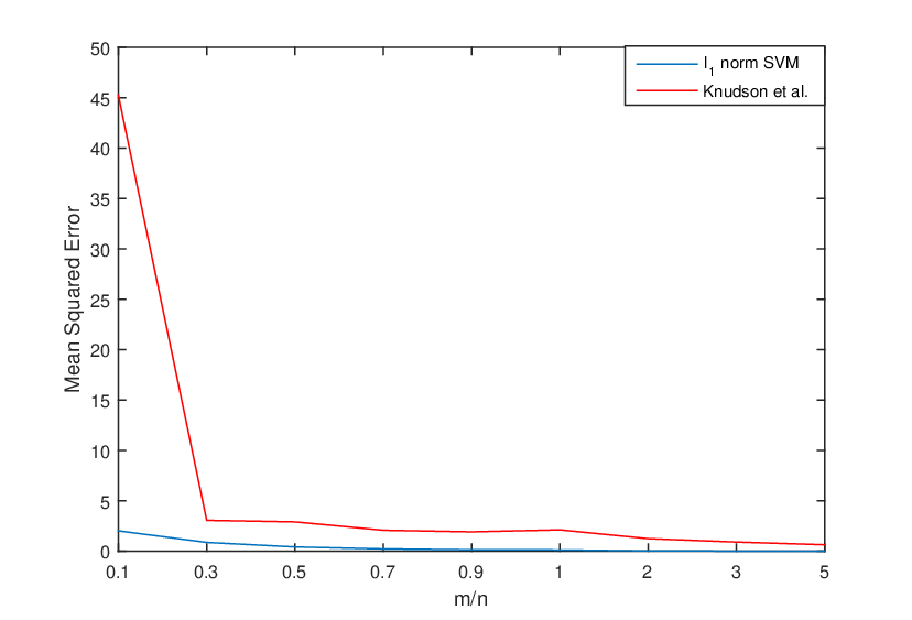
We chose , and generated 30 vectors at random. Then we generated measurements of the form where are normally distributed. Then we applied the algorithm proposed in the previous section, that is, carrying out the minimization in (40) and then truncating the resulting to the dominant components by magnitude.
Figure 2 shows a comparison of the error for our method versus that for the method proposed in [21], for one of the randomly generated -sparse vectors. It is evident that our method ourperforms the latter. This can perhaps be attributed to replacing the conventional SVM as in [21] with the modification in (40). Figure 3 shows the number of correctly recovered components as a function of , for one of the randomly generated -sparse vectors. Figure 4 shows the box plot of the mean square error as a function of over all random repetitions of this experiment. The small horizontal lines show the maximum and minimum error, while the boxes display the 25th and 75th percentiles. Note that, in OBCS, it is meaningful to have .


8 Discussion
In this paper, the problem of one-bit compressed sensing (OBCS) has been formulated as a problem in probably approximately correct (PAC) learning theory. In particular, it has been shown that the VC-dimension of the set of half-spaces in generated by -sparse vectors is bounded by . Therefore, in principle at least, the OBCS problem can be solved using only samples. This is possible in principle even when the measurements are corrupted by noise. However, in general, it is NP-hard to find a consistent algorithm when measurements are free from noise, and to find an algorithm that minimizes empirical risk when measurements are noisy. We proposed a modification of the -norm support vector machine as a feasible alternative, and illustrated that our approach outperforms earlier algorithms in the literature.
One of the main advantages of formulating OBCS as a problem in PAC learning is that extending these results to the case where the samples (or as the case may be) are not i.i.d. essentially “comes for free.” It is now known that, if a concept class has finite VC-dimension, then empirical means converge to their true values not only for i.i.d. samples (or as the case may be), but also when this sequence forms an ergodic process; see [35], which builds on an earlier result in [36] for -mixing processes. However, in order to be useful in OBCS, it is not enough to know this. One must also have expicit estimates of the rate at which empirical means converge to their true values, or what is called the learning rate here. Such estimates are provided in [37]. As it is fairly straight-forward to adapt the various theorems given here to the case of -mixing processes using the above-mentioned results, the details are omitted.
References
- [1] M. Elad, Sparse and Redundant Representations: From Theory to Applications in Signal and Image Processing. Springer-Verlag, New York, 2010.
- [2] S. Foucart and H. Rauhut, A Mathematical Introduction to Compressive Sensing. Springer-Verlag, 2013.
- [3] I. Rish and G. Grabarnik, Sparse Modeling: Theory, Algorithms, and Applications. Boca Raton, FL: CRC Press, Taylor & Francis Group, 2015.
- [4] T. Hastie, R. Tibshirani, and M. Wainwright, Statistical Learning with Sparsity: The Lasso and Generalizations. Boca Raton, FL: CRC Press, Taylor & Francis Group, 2015.
- [5] Y. C. Eldar and G. Kutyniok, Eds., Compressed Sensing: Theory and Applications. Cambridge, UK: Cambridge University Press, 2012.
- [6] M. A. Davenport, M. F. Duarte, Y. C. Eldar, and G. Kutyniok, “Introduction to compressed sensing,” in Compressed Sensing: Theory and Applications, Y. C. Eldar and G. Kutyniok, Eds. Cambridge, UK: Cambridge University Press, 2012, pp. 1–68.
- [7] S. Negabhan, P. Ravikumar, M. J. Wainwright, and B. Yu, “A unified framework for high-dimensional analysis of m-estimators with decomposable regularizers,” Statistical Science, vol. 27(4), pp. 538–557, December 2012.
- [8] E. J. Candès and T. Tao, “Decoding by linear programming,” IEEE Transactions on Information Theory, vol. 51(12), pp. 4203–4215, December 2005.
- [9] E. J. Candès, J. Romberg, and T. Tao, “Stable signal recovery from incomplete and inaccurate measurements,” Communications in Pure and Applied Mathematics, vol. 59(8), pp. 1207–1223, August 2006.
- [10] D. L. Donoho, “Compressed sensing,” IEEE Transactions on Information Theory, vol. 52(4), pp. 1289–1306, April 2006.
- [11] ——, “For most large underdetermined systems of linear equations, the minimal -norm solution is also the sparsest solution,” Communications in Pure and Applied Mathematics, vol. 59(6), pp. 797–829, 2006.
- [12] P. T. Boufounos and R. G. Baraniuk, “1-bit compressive sensing,” in Proceedings of the Conference on Information Sciences and Systems, 2008.
- [13] A. Gupta, R. Nowak, and B. Recht, “Sample complexity for 1-bit compressive sensing and sparse classification,” in Proceedings of the International Symposium on Information Theory, 2010.
- [14] P. T. Boufounos, “Greedy sparse signal reconstruction from sign measurements,” in Proceedings of the Asilomar Conference on Signals, Systems, and Computation, 2009.
- [15] D. Needell and J. A. Tropp, “Cosamp: Iterative signal recovery from incomplete and inaccurate samples,” Applied and Computational Harmonic Analysis, vol. 26, no. 3, pp. 301–321, 2008.
- [16] L. Jacques, J. N. Laska, P. T. Boufounos, and R. G. Baraniuk, “Robust 1-bit compressive sensing via binary stable embeddings of sparse vectors,” IEEE Transactions on Information Theory, vol. 59(4), pp. 2082–2102, April 2013.
- [17] B. K. Natarajan, “Sparse approximate solutions to linear systems,” SIAM Journal on Computing, vol. 24, pp. 227–234, 1995.
- [18] Y. Plan and R. Vershynin, “One-bit compressed sensing by linear programming,” Communications on Pure and Applied Mathematics, vol. 66, pp. 1275–1297, 2013.
- [19] A. Ai, A. Lapanowski, Y. Plan, and R. Vershynin, “One-bit compressed sensing with non-Gaussian measurements,” Linear Algebra and Its Applications, vol. 441, pp. 222–239, 2014.
- [20] Y. Plan and R. Vershynin, “Robust 1-bit compressed sensing and sparse logistic regression: A convex programming approach,” IEEE Transactions on Information Theory, vol. 59, no. 1, pp. 482–494, January 2013.
- [21] K. Knudson, R. Saab, and R. Ward, “One-bit compressive sensing with norm estimation,” IEEE Transactions on Information Theory, vol. 62, no. 5, pp. 2748–2758, 2016.
- [22] L. G. Valiant, “A theory of the learnable,” Journal of the ACM, vol. 29(11), pp. 1134–1142, 1984.
- [23] V. N. Vapnik, Statistical Learning Theory. John Wiley, New York, 1998.
- [24] M. Anthony and P. L. Bartlett, Neural Network Learning: Theoretical Foundations. Cambridge University Press, 1999.
- [25] M. Vidyasagar, A Theory of Learning and Generalization. Springer-Verlag, London, 1997.
- [26] ——, Learning and Generalization: With Applications to Neural Networks and Control Systems. Springer-Verlag, London, 2003.
- [27] M. X. Goemans and D. P. Williamson, “Improved algorithms for maximum cut and satisfiability problems using semidefinite programming,” Journal of the ACM, vol. 42, pp. 1115–1145, 1995.
- [28] A. Blumer, A. Ehrenfeucht, D. Haussler, and M. Warmuth, “Learnability and the vapnik-chervonenkis dimension,” Journal of the ACM, vol. 36, no. 4, pp. 929–965, 1989.
- [29] A. Ehrenfeucht, D. Haussler, M. Kearns, and L. Valiant, “A general lower bound on the number of examples needed for learning,” Information and Computation, vol. 82, pp. 247–261, 1989.
- [30] R. M. Dudley, “Central limit theorems for empirical measures,” The Annals of Probability, vol. 6(6), pp. 899–929, 1978.
- [31] N. Sauer, “On the densities of families of sets,” Journal of Combinatorial Theory, Series A, vol. 13, pp. 145–147, 1972.
- [32] N. Natarajan, I. Dhillon, P. Ravikumar, and A. Tewari, “Learning with noisy labels,” Neural Information Processig Systems, vol. 26, 2013.
- [33] P. S. Bradley and O. L. Mangasarian, “Feature selection via concave minimization and support vector machines,” in Machine Learning: Proceedings of the Fifteenth International Conference (ICML ’98). Morgan Kaufmann, San Francisco, 1998, pp. 82–90.
- [34] C. Cortes and V. N. Vapnik, “Support vector networks,” Machine Learning, vol. 20, 1997.
- [35] T. M. Adams and A. B. Nobel, “Uniform convergence of Vapnik-Chervonenkis classes under ergodic sampling,” The Annals of Probability, vol. 38, no. 4, pp. 1345–1367, 2010.
- [36] A. Nobel and A. Dembo, “Rates of uniform convergence of empirical means with mixingprocesses,” Statistics & Probability Letters, vol. 17, pp. 169–172, 1993.
- [37] R. L. Karandikar and M. Vidyasagar, “Rates of uniform convergence of empirical means with mixingprocesses,” Statistics & Probability Letters, vol. 58, pp. 297–307, 2002.