Edge switching transformations of quantum graphs
Abstract
Discussed here are the effects of basics graph transformations on the spectra of associated quantum graphs. In particular it is shown that under an edge switch the spectrum of the transformed Schrödinger operator is interlaced with that of the original one. By implication, under edge swap the spectra before and after the transformation, denoted by and correspondingly, are level-2 interlaced, so that . The proofs are guided by considerations of the quantum graphs’ discrete analogs.
1 Statement of the main result
Quantum graphs are linear, network-shaped structures of vertices connected by edges, with a Schrödinger like operator suitably defined on functions supported on the edges. Such systems were studied by Linus Pauling as simplified models of valance electrons in organic molecules in the 1930s [16]. More recently attention was called to quantum graphs in the context of quantum chaos [13, 14], and they are defined and discussed at great length and detail in review articles and books (see e.g., [6, 15, 4, 17]). In this note, we consider a general compact quantum graph, , whose edges are metrized and of finite lengths belonging to the list . The associated Schrödinger operators act in , may include external potential and possibly also a magnetic potential :
| (1.1) |
The operator’s definition is incomplete without specifying also the boundary conditions (bc) at vertices. They are assumed here to be local, i.e., expressed in terms of linear relations on the limiting values of the function and of its derivatives along the edges which meet at each vertex . The possible choices which ensure self-adjointness are reviewed in detail in, e.g., [15, 4].
Under mild conditions on and the spectrum of the Schrödinger operator is discrete and bounded below, but not above.
It suffices to assume are integrable, but for a more transparent presentation we focus on the case these are piecewise continuous [4].
This spectrum of is unaffected by the operation of edge splitting, through the insertion of a vertex of degree with Kirchhoff boundary conditions. These require to be continuous at having there directional derivatives satisfying:
| (1.2) |
(To avoid confusion: these boundary conditions are not assumed here for the other quantum graph vertices.)
Our purpose here is to discuss the effects on the spectrum of another basic graph transformation, that of edge switching. It is defined in the following extension of a notion which is used in combinatorial graph theory [18].
Definition 1.1.
For a quantum graph with a self-adjoint Schrödinger operator , an edge switch is a transformation in which a pair of edges in exchange the graph designations of one of their end points. Preserved under this exchange are the edge lengths, the local action of along the corresponding edges, and the vertex boundary conditions – up to the corresponding transposition of the functions whose limiting behavior at the two vertices enter the local boundary conditions.
Under an edge switch the collection of the edge lengths remains unchanged. However the spectra will in the generic case be affected.
For example, for quantum graph Laplacians it is shown in [7] that the topology of the quantum graph with rationally independent edge length "can be heard" in the sense of Marc Kac [11]. For clarity let us add that the graph topology may be affected by a switch, but it does not have to. However, regardless of that, and even in case the switch involves two end points which terminate at a common vertex, the spectrum may be affected through the resulting transposition in the boundary conditions.
Edge switch may be combined with the actions of edge splitting and its inverse – the removal of a degree vertex of Kirchhoff boundary conditions. The group generated by these elements includes various other useful graph modifications under which only the total length is preserved. Among those are:
- a.
An edge crossing: a transformation in which a pair of edges are cut at points , , and cross-rewired at these cut points, keeping the action of locally unchanged along the edge segments. The map is done using vertex insertion, with Kirchhoff rules, followed by an edge switch at the inserted vertices, and then removal of the added pair.
- b.
An egde reversal: a mapping in which the parametrization of one of the graph’s edges is reversed, i.e., the potentials and on are replaced by and , with no other change, in particular preserving the graph’s structure, its edge lengths, and the collection of the boundary conditions through which is defined.
- c.
An edge swap: a transformation in which the lengths of the two edges and the action of along them are exchanged while preserving the graph structure and the boundary conditions at all vertices.
- d.
An edge segment exchange: in which a pair of edges exchange mid segments. The mapping is realizable through a pair of edge crossings.
It may be noted that the graph topology, which is not preserved under a generic edge switch, is preserved under any of the last three operations.
The main result reported here is a statement constraining the difference between the quantum graph’s spectra before and after any of the above operations. We use the following terminology.
Definition 1.2.
Two non-decreasing sequences and are said to be degree- interlaced if for any
| (1.3) |
In case the sequences are more simply said to be interlaced.
The above is a symmetric relation. Eq. (1.3) may be equivalently expressed by saying that the spectral shift is uniformly bound by , i.e., for all
| (1.4) |
where and are the counting functions
| (1.5) |
Following is our main result.
Theorem 1.3.
Let be a quantum graph, which need not be connected, with a self-adjoint Schrödinger operator of the form (1.1). Then under any edge switch the spectra before and after the transformation are interlaced (at degree ).
An immediate consequence is that under each of the other transformations mentioned above the spectra before and after the transformation are degree- interlaced, with
| (1.6) |
Further implications, and related research questions, are discussed at the end of the article.

The notions discussed above can also be considered in the context of finite discrete graphs, an example of which is depicted in Fig. 1. The discrete Hamiltonian is given by a hermitian matrix whose off diagonal terms are of the form
| (1.7) |
with the adjacency matrix of the graph plus an additional potential on the diagonal and representing the single step integral of the vector potential . The role which for quantum graphs is played by edges is assumed here by chains of vertices of . The end points of any chain are its extremal points of degree 2. The discrete analog of the quantum graph’s vertices are therefore the connected clusters of points with .
Using the above as a dictionary, the different notions of graph transformations have a natural extension to the discrete graph case, and so does Theorem 1.3.
2 A pair of relevant finite-rank perturbation principles
It is somewhat instructive to consider first the discrete version, which is what we shall do. As a preliminary observation, let us note that for any edge switch the difference is an operator of rank at most . E.g., the switch of the two edges highlighted in Fig. 1, affect only the matrix elements of within the dimensional block spanned by the vectors .
By the following finite-rank perturbations principle (cf. [19]) any low rank perturbation has only a limited effect on the spectral counting function
| (2.1) |
Lemma 2.1.
Let be a pair of self adjoint operators, with of discrete spectrum which is bounded below and of a finite rank. Then for any :
| (2.2) |
The quantity is often referred to as the Krein spectral shift.
This already allows to deduce (initially for the discrete case)
a weaker version of Theorem 1.3, with (1.6) replaced by times as large spectral shift bounds.
One can do a bit better using the monotonicity of the spectral function under positive perturbations, and the fact that and agree on the subspace of functions which vanish at and . For that, one may consider the two families of operators
| (2.3) |
The key observation now is that as increases from to the spectral counting functions and can only decrease, but by not more than , and for each
| (2.4) |
This allows to deduce that
| (2.5) |
which is a step closer to our claim.
For the tighter bound which is stated in Theorem 1.3 we shall use the following comparison principle.
Lemma 2.2.
For any pair of self adjoint operators and , with of finite rank, and a unitary matrix such that (equivalently ) the spectra of and are intertwined to degree , i.e. for all
| (2.6) |
Proof.
The relation between the two operators can be rewritten as
| (2.7) |
with . The key observation now is that
| (2.8) |
Hence, in the spectral decomposition
| (2.9) |
the number of strictly positive eigenvalues is at most , and so is the number of strictly negative eigenvalues. (In the present case the two are equal, due to the antisymmetry, but it is the above property which matters.)
Therefore adding is equivalent to the addition, one at a time, of operators of rank . In this process, for each the spectral counting function changes by at most steps of and at most steps of . Thus the net spectral shift is bounded by . ∎
3 The discrete graph case
The argument which will be employed for the optimal uniform spectral shift bound (see Fig. 3) starts from a split of the graph at the two points and , in a manner indicated in Fig. 2.
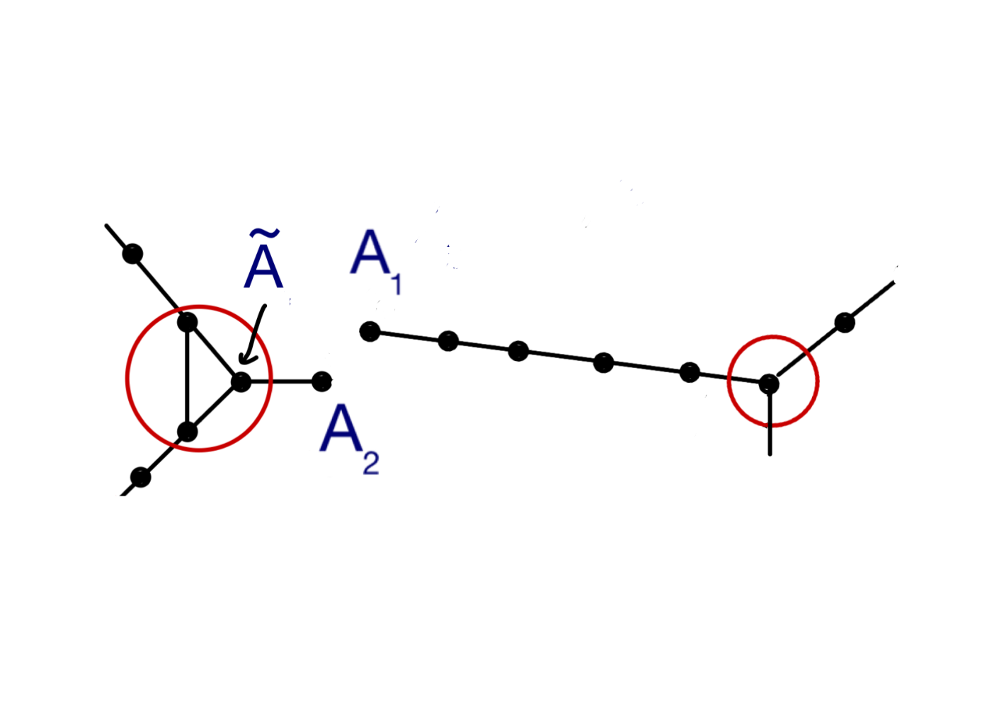
Proof of Theorem 1.3 – the discrete case.
Consider the discrete analogue of the quantum graph which is obtained by splitting the end points of the edges which are to be switched, in a manner indicated in Fig. 2. Denoting by the original finite-dimensional Hilbert space and by the one corresponding to the enlarged graph. The latter is isomorphic to the direct sum . To the operator on , we associate the operator on through the following choices: i) The two operators coincide within the subspace which does not involve the end points and , ii) The matrix element of between and its neighbor along the edge equals times that of between and that neighbor. iii) The matrix element of between and the vertex site is again the product of and the corresponding matrix element of . And finally iv) . Similar convention will be applied at the endpoint with which is to be switched. Consider now the one parameter family of operators
| (3.1) |
Denoting by the operator which transposes , we find:
| (3.2) |
This difference is rank and antisymmetric with respect to the transposition . Lemma 2.2 thus implies that
| (3.3) |
By an orthogonal change of basis in the subspace to , one realizes that on is unitarily equivalent to on a space equivalent to with a - independent rank- operator which is purely off diagonal in the above block decomposition of . I.e., denoting by the orthogonal projection onto the -component of and by , one has . Consequently through an application of the Schur complement formula, for any :
| (3.4) |
and the same applies to . Hence, the spectral shift under edge switch is bounded by one as claim. ∎
4 Proof of the main result
While Theorem 1.3 addresses the spectral shift caused by an edge switch, it is convenient to regard this transformation as a limiting case of an edge crossing. More specifically, let and be a pair of edges whose end points are to be switched. Splitting the edges through the insertion of vertices located at a distance from the corresponding endpoints, with the Kirchhoff boundary conditions on the inserted vertices leaves the spectrum of Hamiltonian invariant. Crossing the edges at the split points results in a new Hamiltonian which we denote by . As this Hamiltonian converges in norm resolvent sense to the Hamiltonian of the edge switch dealt with in Theorem 1.3. This implies the convergence of the counting functions for almost all . It therefore suffices to focus in the proof on the spectral shift under an edge crossing transformation.
Proof of Theorem 1.3 – continuum case, for edge crossing.
With Kirchhoff boundary conditions at the above described edge insertion sites on the chosen pair of edges, the insertion in essense leaves the Hamiltonian invariant. More precisely, it causes no change in the spectrum. However, changing the boundary conditions there to Dirichlet one obtains a different Hamiltonian which we denote by .
As a tool in the proof we will work with the spectral shift resulting from this change:
| (4.1) |
where stands for the number of eigenvalues of strictly below .
Let stand for the Hamiltonian in which the two edges are crossed at the two inserted vertices. By the additivity of the spectral shift, the quantity of interest can therefore be written as
| (4.2) |
Since we assumed the quantum graph to be compact, the spectral shift functions are piecewise constant with only countably many discontinuities. It therefore remains to bound the spectral shift only for almost every .
The resolvents of the original Hamiltonian and the Dirichlet-decoupled operator are related by the Krein formula
| (4.3) |
which involves the gamma field and the Weyl function corresponding to this change of boundary conditions [1]. The latter is a matrix-valued Herglotz function of the spectral parameter . The Weyl function’s boundary values exist for almost all . Since the graph is compact, these boundary values are self-adjoint , We now recall the result of Behrndt-Malamud-Neidhardt [3, Thm. 4.1] that for almost all the spectral shift is given by
| (4.4) |
where is the imaginary part of the principle value of the complex logarithm. Likewise, the spectral shift for the edge-crossed Hamiltonian is given in terms of its Weyl function . The latter is related to by a unitary transposition which swaps two rows/columns,
| (4.5) |
Consequently, for almost every
| (4.6) |
Since the difference is rank two and antisymmetric with respect to , Lemma 2.2 applies, and implies that the spectral shift is bounded by one. ∎
5 Discussion
A few comments are in order.
- A common feature of the transformations considered here is that they do not affect the asymptotic rate of growth of the spectrum. This follows from Weyl’s semi-classical assymptotic formula [20] (see also [9]):
| (5.1) | |||||
and the fact that the sum of edge lengths is preserved under the transformations considered here.
- Given a quantum graph and a list of distinct lengths
there are different arrangements of the lengths over the edges.
Denote by the set of the corresponding quantum graphs, at zero potential but with some fixed boundary conditions.
This
provides an ensemble of quantum graphs with spectra of the same mean spectral density and a common structure of periodic orbits. What would be the spectral statistics for this ensemble? How will it depend on the underlying common structure?
- For pairs of quantum graphs
we can define the (discrete) distance as the smallest number of elementary swaps by which may be transformed to .
Thus we can define an adjacency relation on between quantum graphs at distance . This in turn defines a d-regular "meta-graph" with the quantum graphs as vertices, each with the degree . A random walk on corresponds to a succession of elementary swaps which are chosen at random with equal probability at each step. Since is d-regular, the random walk is ergodic and covers uniformly after sufficiently long "time". This process is the discrete version of Dyson’s Brownian motion approach to spectral statistics [5], and it is discussed at length in [10] for a different class of matrix ensembles.
- A related subject for future research is the systematic study of correlations between different spectra and their dependence on the distance between the graphs.
- A possible tool for further insights on the spectral shift, and also an object of intrinsic interest (cf. [2]) is the question how are nodal counts affected by edge swapping and the other transformations discussed here.
i) ii)
- Length swapping can be easily implemented in experimental simulations of quantum graphs by networks of RF wave-guides [8].
Note added in proof: After the submission of the paper it was called to our attention that an alternative protocol for the edge switch can be based on the vertex gluing operation, which was discussed in [4, Thm. 3.1.10] and in [12, Thm. 1]. Using it, an edge switch can be obtained through vertex gluing followed by un-gluing into the modified graph configuration. Each step produces a spectral shift of at most one, but in different direction. The spectral shift bounds presented here are not improved by this comment, but it does offer another useful perspective. We thank Gregory Berkolaiko, Pavel Kurasov and Sergey Naboko for alerting us to this point of view.
Acknowledgements
We thank Chris Joyner, and Rami Band for useful suggestions and corrections, and Mor Rozner for earlier numerical simulations which have guided us towards tighter results. The work of MA was supported in part by the NSF grant DMS-1613296 and the Weston Visiting Professorship at the Weizmann Institute. He thanks the Faculty of Mathematics and Computer Sciences and the Faculty of Physics at WIS for the hospitality enjoyed there.
References
- [1] Sergio Albeverio and Konstantin Pankrashkin, A remark on Krein’s resolvent formula and boundary conditions. J. Phys A 38, 4859-4864 (2005).
- [2] Rami Band, Gregory Berkolaiko, Hillel Raz and Uzy Smilansky, The number of nodal domains on quantum graphs as a stability index of graph partitions Comm. Math. Phys. 311,815-838 (2012).
- [3] Jussi Behrndt, Mark M. Malamud, and Hagen Neidhardt, Scattering matrices and Weyl functions. Proceedings of the London Mathematical Society 97, 568-598 (2008).
- [4] Gregory Berkolaiko and Peter Kuchment, Introduction to Quantum Graphs, AMS Mathematical Surveys and Monographs 186 (2012).
- [5] Freeman J. Dyson Statistical theory of the energy levels of complex systems I, II and III J. Math. Phys. 3 140 157 and 166 (1962).
- [6] Sven Gnutzmann and Uzy Smilansky, Quantum Graphs: Applications to Quantum Chaos and Universal Spectral Statistics. Advances in Physics 55 527-625 (2006).
- [7] Boris Gutkin and Uzy Smilansky, Can One Hear the Shape of a Graph? J. Phys A.31, 6061-6068 (2001).
- [8] Oleh Hul, Szymon Bauch, Prot Pakoski, Nazar Savytskyy, Karol Zyczkowski and Leszek Sirko, Experimental simulation of quantum graphs by microwave networks, Physical Review E 69, 056205 (2004).
- [9] Dirk Hundertmark, Elliott H. Lieb , Larry E. Thomas. A sharp bound for an eigenvalue moment of the one-dimensional Schrödinger operator. Adv. Theor. Math. Phys. 2, 719-731 (1998).
- [10] Christopher H. Joyner and Uzy Smilansky Spectral statistics of Bernoulli matrix ensembles random walk approach (I) J. Phys. A: Math. Theor. 48, 255101 (2015).
- [11] Mark Kac, Can One Hear the Shape of a Drum?, American Mathematical Monthly, 73, 1-23 (1966).
- [12] Pavel Kurasov, Gabriela Malenová and Sergei Naboko, Spectral gap for quantum graphs and their edge connectivity. J. Phys. A 46, 275309 (2013).
- [13] Tsampikos Kottos and Uzy Smilansky, Quantum Chaos on Graphs Phys. Rev. Lett. 79,4794- 4797, (1997).
- [14] Tsampikos Kottos and Uzy Smilansky, Periodic orbit theory and spectral statistics for quantum graphs Annals of Physics 274, 76-124 (1999).
- [15] Peter Kuchment, Quantum graphs: an introduction and a brief survey, pp.291 - 314 in "Analysis on Graphs and its Applications", Proc. Symp. Pure. Math., AMS 2008.
- [16] Linus Pauling: The Diamagnetic Anisotropy of Aromatic Molecules, The Journal of Chemical Physics 4, 673-677 (1936).
- [17] Olaf Post, Spectral analysis on graph-like spaces, Lecture Notes in Mathematics 2039, Springer 2012.
- [18] J.J. Seidel, Graphs and two-graphs. In: Proc. Fifth Southeastern Conference on Combinatorics, Graph Theory and Computing (Boca Raton, FL., 1974), Congressus Numerantium X, Utilitas.
- [19] Barry Simon, Spectral analysis of rank one perturbations and applications, in “CRM Proceedings and Lecture Notes,” Vol. 8, pp. 109-149 (1995).
- [20] Hermann Weyl, Das asymptotische Verteilungsgesetz der Eigenwerte linearer partieller Differentialgleichungen (mit einer Anwedung auf die Theorie der Hohlraumstrahlung), Math. Ann. 71 441-479 (1912) .