General Nonlinear Stochastic Systems Motivated by Chemostat Models: Complete Characterization of Long-Time Behavior, Optimal Controls, and Applications to Wastewater Treatment

Dang H. Nguyen ^†^†thanks: Department of Mathematics University of Alabama Tuscaloosa, AL 35401, dangnh.maths@gmail.com. The research of this author was supported in part by the National Science Foundation under grant DMS-1853467. Nhu N. Nguyen ^†^†thanks: Department of Mathematics, Wayne State University, Detroit, MI 48202, nhu.math.2611@gmail.com. The research of this author was supported in part by the National Science Foundation under grant DMS-1710827. George Yin ^†^†thanks: Department of Mathematics, Wayne State University, Detroit, MI 48202, gyin@wayne.edu. The research of this author was supported in part by the National Science Foundation under grant DMS-1710827.

Abstract

This paper focuses on a general class of systems of nonlinear stochastic differential equations, inspired by stochastic chemostat models. In the first part, the system is formulated as a hybrid switching diffusion. A complete characterization of the asymptotic behavior of the system under consideration is provided. It is shown that the long-term properties of the system can be classified by using a real-valued parameter $\lambda$ . If $\lambda\leq 0$ , the bacteria will die out, which means that the process does not operate. If $\lambda>0$ , the system has an invariant probability measure and the transition probability of the solution process converges to that of the invariant measure. The rate of convergence is also obtained. One of the distinct features of this paper is that the critical case $\lambda=0$ is also considered. Moreover, numerical examples are given to illustrate our results. In the second part of the paper, controlled diffusions with a long-run average objective function are treated. The associated Hamilton-Jacobi-Bellman (HJB) equation is derived and the existence of an optimal Markov control is established. The techniques and methods of analysis in this paper can be applied to many other stochastic Kolmogorov systems.

Keywords. Switching diffusion, chemostat model, ergodicity, wastewater treatment.

1 Introduction

We consider a class of systems of nonlinear stochastic differential equations. The motivation stems from the pressing need of the treatment of chemostat models that are a laboratory apparatus used for the continuous culture of microorganism, which is a technique introduced by Novick and Szilard in [30]. This technique plays an important role in microbiology, biotechnology, and population biology, and is perhaps the best laboratory idealization of nature for population studies [37]. Chemostats are also used as microcosms in ecology [6, 31] and evolutionary biology [10, 21], as well as in wastewater treatment based on chemostat models [7, 13, 16, 22, 39], which has led to numerous research inventions. Since 1950’s, much attention has been devoted to modeling and analyzing chemostat problems; see [12, 17, 18, 34] and references therein.

The dynamics of the process can be modeled in the general form by a system of ordinary differential equations

\begin{cases}\begin{aligned} \dfrac{dS(t)}{dt}=&\dfrac{S_{0}-f_{0}(S(t))}{\theta}-X(t)f_{1}\big(S(t),X(t)\big),\\ \dfrac{dX(t)}{dt}=&X(t)\left(f_{2}\big(S(t),X(t)\big)-k_{d}-\dfrac{1+R}{\theta}\right),\end{aligned}\end{cases}

(1.1)

where $S(t),X(t)$ are the substrate concentration and the bacterial concentration, respectively; $S_{0}$ and $f_{0}(S)$ are the input concentration and the decay rate of the substrate, respectively; $\frac{1}{\theta}$ is the dilution rate (or equivalently, $\theta$ is the mean residence time), $k_{d}$ is the death rate of $X$ and $R$ is the recycle ratio; $f_{1}(S,X)$ is the consumption rate and $f_{2}(S,X)$ is the growth rate of the bacteria. The formulation in (1.1) is much more general than the existing models. The readers can find works on the specialized forms of the models with specific forms of the functions $f_{0},f_{1},f_{2}$ in [8, 18, 40, 41, 32] and references therein.

To better reflect the reality, effort has been devoted to stochastic systems to take into account the effect of environmental perturbations [19, 36]. A fundamental problem is the long-term behavior of the system. However, the dynamic behaviors have not been fully understood to the best our knowledge. The asymptotic features of the systems and important information such as the wash-out time have not been fully understood to date. In contrast to the existing work, we develop new approaches to carefully analyze the corresponding systems.

Considering the system in a fluctuating environment, we may assume that the dynamics are perturbed by a white noise. Then, we have a stochastic counterpart of (1.1),

\begin{cases}\begin{aligned} dS(t)=&\left(\dfrac{S_{0}-f_{0}\big(S(t)\big)}{\theta}-X(t)f_{1}\big(S(t),X(t)\big)\right)dt+\sigma_{1}S(t)dW_{1}(t),\\ dX(t)=&X(t)\left(f_{2}\big(S(t),X(t)\big)-k_{d}-\dfrac{1+R}{\theta}\right)dt+\sigma_{2}X(t)dW_{2}(t),\end{aligned}\end{cases}

(1.2)

where $W_{1}(t)$ and $W_{2}(t)$ are two independent real-valued Brownian motions. However, it has been recognized that the formulation above is not able to capture some important features of the underlying process. More often than not, in addition to the Brownian type perturbations, there are also abrupt changes in the environment that cannot be described by continuous perturbations. An effective way to model these discrete event perturbations is to use a Markov chain with a finite state space. Suppose that the coefficients $f_{0},f_{1},f_{2},k_{d}$ and the intensities of the white noises depend on $\alpha(t)$ , a random switching process having a finite state space. Then we have a more general system

\begin{cases}\begin{aligned} dS(t)=&\left(\dfrac{S_{0}-f_{0}(S(t),\alpha(t))}{\theta}-X(t)f_{1}\big(S(t),X(t),\alpha(t)\big)\right)dt+\sigma_{1}(\alpha(t))S(t)dW_{1}(t),\\ dX(t)=&X(t)\left(f_{2}\big(S(t),X(t),\alpha(t)\big)-\widetilde{k}_{d}(\alpha(t))\right)dt+\sigma_{2}(\alpha(t))X(t)dW_{2}(t),\end{aligned}\end{cases}

(1.3)

where $\widetilde{k}_{d}(\alpha(t)):=k_{d}(\alpha(t))+\frac{1+R}{\theta}$ , $\alpha(t)$ is a Markov chain with state space $\mathcal{M}=\{1,\dots,m_{0}\}$ and generator $Q=(q_{kl})_{m_{0}\times m_{0}}$ , and $\alpha(t)$ is independent of the Brownian motions so that

\begin{array}[]{ll}&\displaystyle\mathbb{P}\{\alpha(t+\Delta)=j|\alpha(t)=i,\alpha(s),s\leq t\}=q_{ij}\Delta+o(\Delta)\text{ if }i\neq j\ \hbox{ and }\\ &\displaystyle\mathbb{P}\{\alpha(t+\Delta)=i|\alpha(t)=i,\alpha(s),s\leq t\}=1+q_{ii}\Delta+o(\Delta).\end{array}

(1.4)

The models to be considered in this paper belong to the class of stochastic Kolmogorov systems, which is a class of dynamic systems used extensively in ecological, biological, and environment modeling. Two long standing and fundamental questions concerning Kolmogorov systems are: (i) Under what conditions do populations persist or go extinct? (ii) When do interacting species coexist? The answers to these questions are essential for guiding conservation efforts. Our current paper is one of them along this line. In the literature, much effort has been devoted to such systems. A common approach is to use Lyapunov functions, which gives only sufficient conditions that are nowhere near necessary, and are not sharp. In addition, there is no systematic way of finding the Lyapunov functions. The analysis in this work is based on a completely different approach (used in [4, 33, 15]), which requires treating the systems by looking at the boundary. While sharp results for a very general class of stochastic systems have been obtained in [4], some of their conditions are not always satisfied for our model. The proofs for persistence and extinction therefore require some delicate treatment of the behavior of the process near infinity. In the second part of the paper, we also consider controlled systems to reach the goal of getting optimality under a long-run average performance measure.

The rest of the paper is organized as follows. In Section 2, we prove the existence and uniqueness of positive solutions to (1.3) and (1.4). Then a complete characterization of the asymptotic behavior of the system under consideration is provided. We show that the long-term properties of the system can be classified by using a real-valued parameter $\lambda$ . If $\lambda\leq 0$ , the bacteria will die out; if $\lambda>0$ , the system has an invariant probability measure and the transition probability of the solution process converges to the invariant measure. One of the distinct contributions of this paper is that the critical case $\lambda=0$ is also considered. Some numerical examples are given in Section 3. Section 4 is devoted to the study of the system under ergodic control. Controlled diffusions with random switching can be considered, but the notation will be more complex. To highlight the main ergodic control ideas, we decide to use a simplified model without switching. We obtain the Hamilton-Jacobi-Bellman (HJB) equation and prove the existence and uniqueness of the solution of the HJB equation corresponding to the long-term time-average control problem. Establishing the existence and uniqueness of the solution to the HJB equation is most difficult because the usual conditions for ergodic controlled diffusions are not satisfied in our model. Inspired by the work [2], we use a vanishing discount argument to examine the associated cost and value functions of the corresponding discounted control problem and then to take a limit when the discount factor tends to $0.$ However, the results in the aforementioned book cannot be applied or adopted directly because the conditions in the reference are not satisfied in our setup. More details on this will be given in Section 4. Finally, Section 5 issues some concluding remarks. Although our main motivation comes from chemostat models, the analysis and techniques used can be applied to many other nonlinear ecological and biological systems.

2 Complete Characterization of Long-Time Behavior

This section is devoted to asymptotic properties of the switching diffusion models. We show that the long-term properties of the system can be completely classified by using a real parameter $\lambda$ . In particular, if $\lambda\leq 0$ , the bacteria will die out and we refer to such case as the system being not permanent because it does not work in long term and the efficiency goes to 0. If $\lambda>0$ , the system has an invariant probability measure and the transition probability of the solution process converges to the invariant measure. This is what we refer to as permanence (with the terminology carried over from the study in biological and ecological models). Moreover, we obtain the rate of convergence.

One of the highlights here is that we derive sufficient and necessary conditions for permanence. First, the process under consideration is jointly a Markov Feller process. By using the Lyapunov exponent of $X(t)$ , we then establish the existence of the invariant measure of $(S(t),\alpha(t))$ . Furthermore, under suitable conditions, we obtain the exponential error bounds of the difference of the transition function and that of the invariant measure in the total variation norm.

Throughout this paper, we use the lowercase letters $s$ , $x$ , and $i$ to denote the initial values of $S(t)$ , $X(t)$ , and $\alpha(t)$ , respectively. Note the distinction of $s$ and the input concentration of the substrate $S_{0}$ . To simplify the notation, let

\widehat{k}_{d}=\max_{i\in\mathcal{M}}\{\widetilde{k}_{d}(i)\}\;;\;\check{k}_{d}=\min_{i\in\mathcal{M}}\{\widetilde{k}_{d}(i)\},

and

\widehat{\sigma}_{k}=\max_{i\in\mathcal{M}}\{\sigma_{k}(i)\}\;;\;\check{\sigma}_{k}=\min_{i\in\mathcal{M}}\{\sigma_{k}(i)\},k=1,2.

We denote by $\mathbb{R}_{+}=[0,\infty)$ , $\mathbb{R}^{\circ}_{+}=(0,\infty)$ , $\mathbb{R}_{+}^{2}=[0,\infty)\times[0,\infty)$ , and $\mathbb{R}^{2,\circ}_{+}=(0,\infty)\times(0,\infty)$ . The operator associated with the process $\big(S(t),X(t),\alpha(t)\big)$ , solving (1.3) and (1.4), is given by

\mathcal{L}V(\phi,i)=V_{\phi}(\phi,i)\widetilde{f}(\phi,i)+\frac{1}{2}{\rm tr}[\widetilde{g}(\phi,i)\widetilde{g}^{\top}(\phi,i)V_{\phi\phi}(\phi,i)]+\sum_{j\in\mathcal{M}}q_{ij}V(\phi,j),

(2.1)

where $A^{\top}$ denotes the transpose of $A$ , $\phi=(s,x)$ , $V_{\phi}(\phi,i)$ and $V_{\phi\phi}(\phi,i)$ are the gradient and Hessian of $V(\cdot,i)$ with respect to $\phi$ , $\widetilde{f}$ and $\widetilde{g}$ are the drift and diffusion coefficients of (1.3), respectively. That is,

\begin{array}[]{rl}&\!\!\!\displaystyle\widetilde{f}(\phi,i)=\left(\dfrac{S_{0}-f_{0}(s,i)}{\theta}-xf_{1}(s,x,i),\;\;x\Big(f_{2}(s,x,i)-\widetilde{k}_{d}(i)\Big)\right)^{\top},\\ &\!\!\!\displaystyle\widetilde{g}(\phi,i)={\rm diag}\big(\sigma_{1}(i)s,\sigma_{2}(i)x\big)\in{\mathbb{R}}^{2\times 2},\end{array}

where ${\rm diag}(a,b)$ denotes the diagonal matrix with entries $a$ and $b$ . Note that the particular structure of $\widetilde{g}$ implies that $\widetilde{g}\widetilde{g}^{\top}=\widetilde{g}^{2}$ . In what follows, we write $V(\phi,i)$ and $V(s,x,i)$ interchangeably, whichever is more convenient. We also assume the following conditions throughout.

Assumption 2.1.

Suppose that

•

$W_{1}(t)$ and $W_{2}(t)$ are independent real-valued standard Brownian motions that are independent of the Markov chain $\alpha(t)$ .
•

$S_{0}$ , $\theta$ , $\widetilde{k}_{d}(i)$ , $\sigma_{1}(i)$ , $\sigma_{2}(i)$ are positive constants for each $i\in\mathcal{M}$ .
•

$f_{0}(s,i)$ , $f_{1}(s,x,i)$ , and $f_{2}(s,x,i)$ are locally Lipschitz; $f_{0}(0,i)=f_{1}(0,x,i)=0$ satisfying $\displaystyle\lim_{s\to\infty}f_{0}(s,i)=\infty$ ; $0\leq f_{2}(s,x,i)\leq\kappa_{0}\big(f_{1}(s,x,i)\wedge f_{0}(s,i)\big)$ , $f_{1}(s,x,i)\leq\kappa_{0}(1+s)$ for some $\kappa_{0}>1$ . Moreover, for each $i\in\mathcal{M}$ , $f_{2}(s,x,i)$ is uniformly continuous at $x=0$ (that is, $\lim_{x\to 0}\sup\{|f_{2}(s,x,i)-f_{2}(s,0,i)|\}=0$ ).
•

The Markov chain or its generator $Q=(q_{ij})_{m_{0}\times m_{0}}$ is irreducible, that is for any $i,j\in\mathcal{M}$ , there exist $i=i_{0},i_{1},\dots,i_{n}=j$ such that $q_{i_{k-1},i_{k}}>0$ for $k=1,\dots,n$ .

To start, we state following Theorem, which provides the preliminary results, namely, the existence and uniqueness of the global solution, and the positivity of the solution. The proof is postponed to the Appendix.

Theorem 2.1.

For any $(s,x,i)\in\mathbb{R}_{+}^{2}\times\mathcal{M}$ , there exists a unique global solution to the system (1.3) and (1.4) with initial value $(s,x,i)$ . The three-component process $\{(S(t),X(t),\alpha(t)),t\geq 0\}$ is a Markov-Feller process. Moreover, we have $\mathbb{P}_{s,x,i}\{S(t)>0,t>0\}=1$ and $\mathbb{P}_{s,x,i}\{X(t)=0,t>0\}=1$ if $x=0$ , $\mathbb{P}_{s,x,i}\{X(t)>0,t>0\}=1$ if $x>0$ .

To proceed, we examine the boundary by letting $X(t)=0$ . Let $\widehat{S}(t)$ be the solution to (1.3) with $X(t)=0$ , i.e.,

d\widehat{S}(t)=\dfrac{S_{0}-f_{0}\big(\widehat{S}(t),\alpha(t)\big)}{\theta}dt+\sigma_{1}(\alpha(t))\widehat{S}(t)dW_{1}(t).

(2.2)

Since the drift of (2.2) is negative when $\widehat{S}(t)$ is sufficiently large, and is positive when $\widehat{S}(t)$ is sufficiently small, we can see

\left[\widehat{\cal L}\Big(s+\ln\frac{s}{s+1}\Big)\right](s,i)\leq-1\text{ if }s<\widehat{s}\text{ or }s>\frac{1}{\widehat{s}},

for some $\widehat{s}>0$ being sufficiently small, where $\widehat{\cal L}$ is the operator associated with (2.2). Thus, the hybrid diffusion (2.2) is positive recurrent due to its nondegeneracy (see, e.g., [38, Chapter 4]). Then there exists a unique invariant measure $\pi$ of (2.2). Moreover,

\lim_{t\to\infty}\|\widehat{P}(t,s,i,\cdot)-\pi(\cdot)\|_{TV}=0,(s,i)\in(0,\infty)\times\mathcal{M},

(2.3)

where $\|\cdot\|_{TV}$ is the total variation norm of a measure and $\widehat{P}(t,s,i,\cdot)$ is the transition probability of $(\widehat{S}(t),\alpha(t))$ . Since $\mathbb{P}_{0,i}\{\widehat{S}(t)>0,t>0\}=1$ , (2.3) holds even when $s=0$ .

When $X(t)$ is small, $S(t)$ can be approximated by $\widehat{S}(t)$ . Due to Itô’s formula and the ergodicity of $(\widehat{S}(t),\alpha(t))$ , when $X(t)$ is small, the long-term growth rate $\dfrac{\ln X(t)}{t}$ is approximated by the critical value

\lambda:=\sum_{i\in\mathcal{M}}\int_{\mathbb{R}_{+}^{\circ}}\left(f_{2}(s,0,i)-\widetilde{k}_{d}(i)-\frac{\sigma_{2}^{2}(i)}{2}\right)\pi(ds,i).

(2.4)

As a result, the sign of $\lambda$ determines whether or not $X(t)$ converges to $0$ . A heuristic argument for getting $\lambda$ can be found in [9]. The main results of this section is provided in the next theorem to follow. First, we state an assumption. One of the conditions in Assumption 2.2 will be used in the main theorem.

Assumption 2.2.

Denoting by $\pi_{\alpha}$ the invariant measure of $\alpha(t)$ , assume that one of the following conditions holds.

(1)

For each $i\in\mathcal{M}$ , $f_{2}(s,x,i)$ is non-decreasing in $s$ and non-increasing in $x$ for any $(s,x)\in[0,\infty)\times(0,\infty)$ ;

(2)

\sum_{i\in\mathcal{M}}\left(\limsup_{s\to\infty}f_{2}(s,0,i)-\widetilde{k}_{d}(i)-\frac{\sigma_{2}^{2}(i)}{2}\right)\pi_{\alpha}(i)<0;

(2.5)

(3)

\sum_{i\in\mathcal{M}}\left(\liminf_{s\to\infty}f_{2}(s,0,i)-\widetilde{k}_{d}(i)-\frac{\sigma_{2}^{2}(i)}{2}\right)\pi_{\alpha}(i)>0.

(2.6)

Theorem 2.2.

The following claims hold.

•

If $\lambda<0$ , we have $\lim\limits_{t\to\infty}\dfrac{\ln X(t)}{t}=\lambda$ a.s. and the distribution of $\big(S(t),\alpha(t)\big)$ converges weakly to the unique invariant probability measure $\pi$ if either condition (1) or (2) of Assumption 2.2 holds.

•

If $\lambda=0$ and condition (1) of Assumption 2.2 holds then

\lim_{T\to\infty}\dfrac{1}{T}\mathbb{E}_{s,x,i}\int_{0}^{T}S(t)dt=S_{0}\,\text{ and }\,\lim_{T\to\infty}\dfrac{1}{T}\mathbb{E}_{s,x,i}\int_{0}^{T}X(t)dt=0

(2.7)

under additional conditions that for any $i\in\mathcal{M}$ , $\frac{\partial f_{0}(s,i)}{\partial s}$ and $\frac{\partial f_{2}(s,0,i)}{\partial s}$ exist and are positive, continuous, and $\frac{\partial f_{0}(s,i)}{\partial s}$ is bounded below by a positive constant.

•

If $\lambda>0$ , then there exists an invariant probability measure $\mu^{*}$ on $\mathbb{R}^{2,\circ}_{+}\times\mathcal{M}$ and $\lim_{t\to\infty}\|P(t,s,i,\cdot)-\mu^{*}(\cdot)\|_{TV}=0$ . We assume further that condition (3) of Assumption 2.2 holds, and $\liminf_{s\to\infty}\frac{f_{0}(s,i)}{s^{q}}>0,i\in\mathcal{M}$ for some $q\in(0,1]$ . Then,

(i)

in case $q<1$ ,

\begin{array}[]{rl}&\!\!\!\displaystyle\lim_{t\to\infty}t^{\beta-1}\|P(t,s,x,i,\cdot)-\mu^{*}(\cdot)\|_{TV}=0,\\ &\displaystyle\hskip 130.08621pt\text{ for any }1\leq\beta<\frac{1}{1-q},(s,x,i)\in\mathbb{R}_{+}\times\mathbb{R}^{\circ}_{+}\times\mathcal{M};\end{array}

(ii)

if $q=1$ , there exists a $\widetilde{\gamma}>0$ such that

\lim_{t\to\infty}e^{\widetilde{\gamma}t}\|P(t,s,x,i,\cdot)-\mu^{*}(\cdot)\|_{TV}=0,(s,x,i)\in\mathbb{R}_{+}\times\mathbb{R}^{\circ}_{+}\times\mathcal{M},

(2.8)

where $P(t,s,x,i,\cdot)$ is the transition probability of $\big(S(t),X(t),\alpha(t)\big)$ .

Remark 2.1.

If $\lambda>0$ , it is easy to see that condition (1) of Assumption 2.2 implies the condition (3) in Assumption 2.2. Moreover, most models in the literature consider the case $f_{0}(s)=C_{i}s$ while the coefficients $xf_{1}(s,x,i),xf_{2}(s,x)$ are linear functional response $(f_{j}(s,x,i)=c_{ij}x,j=1,2)$ , Holling type II response $(f_{j}(s,x,i)=\frac{c_{ij}s}{m_{ij}+a_{ij}s},j=1,2)$ , Holling type III response $(f_{j}(s,x,i)=\frac{c_{ij}s^{2}}{(m_{ij1}+a_{ij1}s)(m_{ij2}+a_{ij2}s)},j=1,2)$ , and Beddington-DeAngelis functional response $(f_{j}(s,x,i)=\frac{c_{ij}s}{m_{ij}+a_{ij}s+b_{ij}x},j=1,2)$ etc.; see e.g., [32, 40, 41] and the references therein. It is clear that these functions satisfy Assumption 2.1 and part (1) of Assumption 2.2.

Proof for the case $\lambda=0$ .

We argue by contradiction. Suppose $\big(S(t),X(t),\alpha(t)\big)$ has an invariant probability measure $\mu^{*}$ on $\mathbb{R}^{2,\circ}_{+}\times\mathcal{M}$ . Then, it follows from the ergodicity that for $\mu^{*}$ -almost every initial value $(s,x,i)$ ,

\lim_{T\to\infty}\frac{1}{T}\int_{0}^{T}h\big(S(t),X(t),\alpha(t)\big)dt=\sum_{i^{\prime}\in\mathcal{M}}\int_{\mathbb{R}^{2,\circ}_{+}}h(s^{\prime},x^{\prime},i^{\prime})\mu^{*}(ds^{\prime},dx^{\prime},i^{\prime}),

(2.9)

for any measurable function $h$ that is $\mu^{*}$ -integrable. Since the transition probability density is continuous and positive, the invariant measure $\mu^{*}$ is unique and equivalent to $\widetilde{m}\times\pi_{\alpha}$ where $\widetilde{m}$ is the Lebesgue measure on $\mathbb{R}^{2,\circ}_{+}$ . As a result, if $\mu^{*}(A)=1$ , then $\mathbb{P}_{s,x,i}\big((S(t),X(t),\alpha(t))\in A)\big)=1$ for every $(s,x,i)\in\mathbb{R}^{2,\circ}_{+}\times\mathcal{M},t>0$ , which implies that (2.9) holds for any initial value $(s,x,i)\in\mathbb{R}^{2,\circ}_{+}\times\mathcal{M}$ . By the comparison theorem (see e.g., [14]), we have $\widehat{S}(t)\geq S(t)$ with probability 1 given that $\widehat{S}(0)=S(0)$ . Hence, it follows (1.3), (2.2) and positivity of $S(t)$ , $\widehat{S}(t)$ and additional assumption on $f_{0}(\cdot,\cdot)$ (non-decreasing in $s$ ) that

\limsup_{T\to\infty}\dfrac{1}{T}\mathbb{E}_{s,x,i}\int_{0}^{T}f_{0}(S(t),\alpha(t))dt\leq\limsup_{T\to\infty}\dfrac{1}{T}\mathbb{E}_{s,i}\int_{0}^{T}f_{0}(\widehat{S}(t),\alpha(t))dt\leq S_{0}.

(2.10)

On the other hand, since $\dfrac{\partial f_{0}(s,i)}{\partial s}$ is bounded below by a positive constant and $f_{0}(0,i)=0$ , there exists a $\overline{g}_{1}>0$ such that

\frac{f_{0}(s,i)}{\theta}\geq\overline{g}_{1}s,\ \forall s\geq 0,i\in\mathcal{M}.

(2.11)

Let $0<\overline{p}<\frac{\overline{g}_{1}}{2\widehat{\sigma}_{1}^{2}}$ and $0<\overline{g}_{2}<\frac{(1+\overline{p})\overline{g}_{1}}{4}$ . By Itô’s formula, we obtain that

	$\displaystyle\mathbb{E}_{s,i}$	$\displaystyle e^{\overline{g}_{2}T}\widehat{S}^{1+\overline{p}}(T)$
	$\displaystyle=$	$\displaystyle s^{1+\overline{p}}+\mathbb{E}_{s,i}\int_{0}^{T}e^{\overline{g}_{2}t}(1+\overline{p})\widehat{S}^{\overline{p}}(t)\left(\dfrac{S_{0}-f_{0}\big(\widehat{S}(t),\alpha(t)\big)}{\theta}+\dfrac{\overline{p}\sigma_{1}^{2}(\alpha(t))}{2}\widehat{S}(t)+\dfrac{\overline{g}_{2}}{1+\overline{p}}\widehat{S}(t)\right)dt$
	$\displaystyle\leq$	$\displaystyle s^{1+\overline{p}}+\mathbb{E}_{s,i}\int_{0}^{T}e^{\overline{g}_{2}t}(1+\overline{p})\widehat{S}^{\overline{p}}(t)\left(\dfrac{S_{0}}{\theta}-\dfrac{\overline{g}_{1}}{2}\widehat{S}(t)\right)dt$
	$\displaystyle\leq$	$\displaystyle s^{1+\overline{p}}+\dfrac{\overline{g}_{3}e^{\overline{g}_{2}T}}{\overline{g}_{2}},\;\forall T>0,\text{where }\overline{g}_{3}:=\dfrac{(1+\overline{p})S_{0}}{\theta}\left(\dfrac{2S_{0}}{\theta\overline{g}_{1}}\right)^{\overline{p}}.$

As a consequence, we have

\limsup_{T\to\infty}\mathbb{E}_{s,x,i}S^{1+\overline{p}}(T)\leq\limsup_{T\to\infty}\mathbb{E}_{s,i}\widehat{S}^{1+\overline{p}}(T)\leq\dfrac{\overline{g}_{3}}{\overline{g}_{2}}.

(2.12)

Moreover, we also obtain that

\mathbb{E}_{s,x,i}\big(S(T)+X(T)\big)^{1+\overline{p}}\text{ is uniformly bounded in }T.

(2.13)

Using Itô’s formula again, we have

	$\displaystyle\dfrac{\mathbb{E}_{s,i}\widehat{S}^{1+\overline{p}}(T)}{T}=\dfrac{s^{1+\overline{p}}}{T}$	$\displaystyle+\dfrac{(1+\overline{p})S_{0}}{\theta T}\mathbb{E}_{s,i}\int_{0}^{T}\widehat{S}^{\overline{p}}(t)dt-\dfrac{1+\overline{p}}{\theta T}\mathbb{E}_{s,i}\int_{0}^{T}\widehat{S}^{\overline{p}}(t)f_{0}\big(\widehat{S}(t),\alpha(t)\big)dt$
		$\displaystyle+\dfrac{\overline{p}(1+\overline{p})}{2T}\mathbb{E}_{s,i}\int_{0}^{T}\sigma_{1}^{2}(\alpha(t))\widehat{S}^{1+\overline{p}}(t)dt,$

which together with (2.12) implies that

\limsup_{T\to\infty}\dfrac{1}{T}\mathbb{E}_{s,i}\int_{0}^{T}\widehat{S}^{\overline{p}}(t)f_{0}\big(\widehat{S}(t),\alpha(t)\big)dt\leq\overline{g}_{4},\;\text{for some }\overline{g}_{4}<\infty.

(2.14)

We have from (2.2) and (2.12) that

\lim_{T\to\infty}\dfrac{1}{T}\mathbb{E}_{s,i}\int_{0}^{T}\left(\dfrac{S_{0}}{\theta}-\dfrac{f_{0}\big(\widehat{S}(t),\alpha(t)\big)}{\theta}\right)dt=\lim_{T\to\infty}\dfrac{\mathbb{E}_{s,i}\widehat{S}(T)-s}{T}=0.

Hence

\lim_{T\to\infty}\dfrac{1}{T}\mathbb{E}_{s,i}\int_{0}^{T}f_{0}\big(\widehat{S}(t),\alpha(t)\big)dt=S_{0}.

(2.15)

From (1.3), with standard arguments, we have

\mathbb{E}_{s,x,i}\int_{0}^{T}X(t)f_{1}(S(t),X(t),\alpha(t))dt\leq S_{0}T+s,\;T\geq 0.

Moreover, due to the uniform boundedness (2.13), the linear growth bound of $f_{0}$ and the almost sure convergence (2.9), it follows from the dominated convergence theorem that

\lim_{T\to\infty}\frac{1}{T}\mathbb{E}_{s,x,i}\int_{0}^{T}\left(\dfrac{S_{0}-f_{0}\big(S(t),\alpha(t)\big)}{\theta}\right)dt=\sum_{i^{\prime}\in\mathcal{M}}\int_{\mathbb{R}^{2,\circ}_{+}}\frac{S_{0}-f_{0}(s^{\prime},x^{\prime},i^{\prime})}{\theta}\mu^{*}(ds^{\prime},dx^{\prime},i^{\prime})=:\widehat{g}

(2.16)

From (1.3) and (2.13), we deduces that $\lim_{T\to\infty}\frac{1}{T}\mathbb{E}_{s,x,i}\int_{0}^{T}X(t)f_{1}(S(t),X(t),\alpha(t))dt$ exists (because the two others in (2.17) exist) and

\begin{array}[]{ll}&\!\!\!\displaystyle\lim_{T\to\infty}\frac{1}{T}\mathbb{E}_{s,x,i}\int_{0}^{T}\left(\dfrac{S_{0}-f_{0}\big(S(t),\alpha(t)\big)}{\theta}-X(t)f_{1}\big(S(t),X(t),\alpha(t)\big)\right)dt\\ &\displaystyle\ =\lim_{T\to\infty}\frac{\mathbb{E}_{s,x,i}S(T)-s}{T}=0,\end{array}

(2.17)

where, due to Fatou’s lemma,

\begin{array}[]{rl}&\!\!\!\displaystyle\lim_{T\to\infty}\frac{1}{T}\mathbb{E}_{s,x,i}\int_{0}^{T}X(t)f_{1}\big(S(t),X(t),\alpha(t)\big)dt\\ &\displaystyle\ =\widehat{g}\geq\sum_{i^{\prime}\in\mathcal{M}}\int_{\mathbb{R}^{2,\circ}_{+}}x^{\prime}f_{1}(s^{\prime},x^{\prime},i^{\prime})\mu^{*}(ds^{\prime},dx^{\prime},i^{\prime})>0.\end{array}

We have from (2.15) and (2.16) that

\lim_{T\to\infty}\frac{1}{T}\mathbb{E}_{s,x,i}\int_{0}^{T}\left(f_{0}\big(\widehat{S}(t),\alpha(t)\big)-f_{0}\big(S(t),\alpha(t)\big)\right)dt=\theta\widehat{g},\,s,x\geq 0,i\in\mathcal{M}.

(2.18)

Now, let $H>1$ be a sufficiently large constant satisfying that $\frac{\overline{g}_{4}}{H^{\overline{p}}}\leq\frac{\theta\widehat{g}}{2}.$ Combining with (2.14), we obtain

$\displaystyle\limsup_{T\to\infty}\dfrac{1}{T}\mathbb{E}_{s,x,i}$	$\displaystyle\int_{0}^{T}\boldsymbol{1}_{\{\widehat{S}(t)>H\}}\left(f_{0}\big(\widehat{S}(t),\alpha(t)\big)-f_{0}\big(S(t),\alpha(t)\big)\right)dt$	(2.19)
$\displaystyle\leq$	$\displaystyle\limsup_{T\to\infty}\dfrac{1}{T}\mathbb{E}_{s,x,i}\int_{0}^{T}\dfrac{\widehat{S}^{\overline{p}}(t)}{H^{\overline{p}}}f_{0}\big(\widehat{S}(t),\alpha(t)\big)dt$
$\displaystyle\leq$	$\displaystyle\dfrac{\overline{g}_{4}}{H^{\overline{p}}}\leq\dfrac{\theta\widehat{g}}{2}.$

A consequence of (2.18) and (2.19) is that

\liminf_{T\to\infty}\frac{1}{T}\mathbb{E}_{s,x,i}\int_{0}^{T}\boldsymbol{1}_{\{\widehat{S}(t)\leq H\}}\left(f_{0}\big(\widehat{S}(t),\alpha(t)\big)-f_{0}\big(S(t),\alpha(t)\big)\right)dt\geq\frac{\theta\widehat{g}}{2}.

(2.20)

Since $\frac{\partial f_{0}(s,0,i)}{\partial s}$ is continuous and positive, there exists a $\overline{g}_{5}^{H}<\infty$ such that

f_{0}(s_{1},i)-f_{0}(s_{2},i)\leq\overline{g}_{5}^{H}(s_{1}-s_{2}),\;\forall 0\leq s_{2}\leq s_{1}\leq H,i\in\mathcal{M}.

Thus, (2.20) implies that

\liminf_{T\to\infty}\frac{1}{T}\mathbb{E}_{s,x,i}\int_{0}^{T}\boldsymbol{1}_{\{\widehat{S}(t)\leq H\}}\left(\widehat{S}(t)-S(t)\right)dt\geq\frac{\theta\widehat{g}}{2\overline{g}_{5}^{H}}.

(2.21)

Similarly, there exists a $\overline{g}_{6}^{H}>0$ such that

f_{2}(s_{1},0,i)-f_{2}(s_{2},0,i)\geq\overline{g}_{6}^{H}(s_{1}-s_{2}),\text{ for any }0\leq s_{2}\leq s_{1}\leq H,i\in\mathcal{M}.

Hence, combining with $f_{2}(s,x,i)$ being non-increasing in $x$ , we obtain

f_{2}(s_{1},0,i)-f_{2}(s_{2},x,i)\geq\overline{g}_{6}^{H}(s_{1}-s_{2})\;\forall x\geq 0,0\leq s_{2}\leq s_{1}\leq H,i\in\mathcal{M}.

(2.22)

As a consequence of (2.21) and (2.22),

	$\displaystyle\lim_{T\to\infty}$	$\displaystyle\frac{1}{T}\mathbb{E}_{s,x,i}\int_{0}^{T}\left(f_{2}\big(\widehat{S}(t),0,\alpha(t)\big)-f_{2}\big(S(t),X(t),\alpha(t)\big)\right)dt$
	$\displaystyle\geq$	$\displaystyle\lim_{T\to\infty}\frac{1}{T}\mathbb{E}_{s,x,i}\int_{0}^{T}\boldsymbol{1}_{\{\widehat{S}(t)\leq H\}}\left(f_{2}\big(\widehat{S}(t),0,\alpha(t)\big)-f_{2}\big(S(t),X(t),\alpha(t)\big)\right)dt$
	$\displaystyle\geq$	$\displaystyle\overline{g}_{6}^{H}\liminf_{T\to\infty}\frac{1}{T}\mathbb{E}_{s,x,i}\int_{0}^{T}\boldsymbol{1}_{\{\widehat{S}(t)\leq H\}}\left(\widehat{S}(t)-S(t)\right)dt$
	$\displaystyle\geq$	$\displaystyle\frac{\overline{g}_{6}^{H}\theta\widehat{g}}{2\overline{g}_{5}^{H}}.$

Therefore, we obtain that

$\displaystyle\sum_{i^{\prime}\in\mathcal{M}}$	$\displaystyle\int_{\mathbb{R}_{+}^{2,\circ}}\left(f_{2}(s^{\prime},x^{\prime},i^{\prime})-\widetilde{k}_{d}(i)-\frac{\sigma_{2}^{2}(i)}{2}\right)\mu^{*}(ds^{\prime},dx^{\prime},i^{\prime})$	(2.23)
$\displaystyle=$	$\displaystyle\lim_{T\to\infty}\frac{1}{T}\mathbb{E}_{s,x,i}\int_{0}^{T}\left(f_{2}\big(S(t),X(t),\alpha(t)\big)-\widetilde{k}_{d}(\alpha(t))-\dfrac{\sigma_{2}^{2}(\alpha(t))}{2}\right)dt$
$\displaystyle\leq$	$\displaystyle\lim_{T\to\infty}\frac{1}{T}\mathbb{E}_{s,x,i}\int_{0}^{T}\left(f_{2}\big(\widehat{S}(t),0,\alpha(t)\big)-\widetilde{k}_{d}(\alpha(t))-\dfrac{\sigma_{2}^{2}(\alpha(t))}{2}\right)dt-\frac{\overline{g}_{6}^{H}\theta\widehat{g}}{2\overline{g}_{5}^{H}}$
$\displaystyle\leq$	$\displaystyle\lambda-\frac{\overline{g}_{6}^{H}\theta\widehat{g}}{2\overline{g}_{5}^{H}}=-\frac{\overline{g}_{6}^{H}\theta\widehat{g}}{2\overline{g}_{5}^{H}}.$

By (1.3), Itô’s formula, the ergodicity, and (2.23), we have

	$\displaystyle\lim_{T\to\infty}\dfrac{\ln X(T)}{T}=$	$\displaystyle\lim_{T\to\infty}\dfrac{1}{T}\left(X(0)+\int_{0}^{T}\sigma_{2}(\alpha(t))dW_{2}(t)\right)$
		$\displaystyle+\lim_{T\to\infty}\dfrac{1}{T}\int_{0}^{T}\left(f_{2}\big(S(t),X(t),\alpha(t)\big)-\widetilde{k}_{d}(\alpha(t))-\dfrac{\sigma_{2}^{2}(\alpha(t))}{2}\right)dt$
	$\displaystyle\leq$	$\displaystyle-\frac{\overline{g}_{6}^{H}\theta\widehat{g}}{2\overline{g}_{5}^{H}}<0\ \text{ a.s.}$

As a result,

\mathbb{P}_{s,x,i}\left\{\lim_{T\to\infty}X(T)=0\right\}=1,

which contradicts the assumption that the process has an invariant probability measure on $\mathbb{R}^{2,\circ}_{+}\times\mathcal{M}$ . Moreover, $\pi\times\delta^{*}$ is the unique invariant measure of $\big(S(t),\alpha(t),X(t)\big)$ on $\mathbb{R}_{+}\times\mathcal{M}\times\mathbb{R}_{+}$ , where $\delta^{*}$ is the Dirac measure with mass at $0$ . Consider the empirical measure

\Pi^{s,x,i}_{t}(\cdot)=\dfrac{1}{t}\int_{0}^{t}\mathbb{P}_{s,x,i}\{(S(s),X(s),\alpha(s))\in\cdot\}ds.

In view of (2.13), the family $\{\Pi^{s,x,i}_{t}(\cdot),t\geq 0\}$ is tight for each $(s,x,i)\in\mathbb{R}^{2}_{+}\times\mathcal{M}$ . It is well-known (see e.g., [15] and [33]) that any weak limit of $\Pi^{s,x,i}_{t}(\cdot)$ as $t\to\infty$ is an invariant probability measure of $\big(S(t),\alpha(t),X(t)\big)$ . Since $\pi\times\delta^{*}$ is the unique invariant probability measure and we have the boundedness of $\mathbb{E}_{s,x,i}\big(S(t)+X(t)\big)^{1+\overline{p}}$ in (2.13), we can easily obtain (2.7). ∎

Proof for the case $\lambda>0$ .

Proof of the convergence in total variation of transition probability to an invariant measure is straightforward. Applying [4, Theorem 4.4], with $W(s,x,i)=s+x$ and $V(s,x,i)=\ln\frac{x}{x+1}$ we obtain the persistence of $X(t)$ and the existence of an invariant probability measure of $(S(t),X(t),\alpha(t))$ on $\mathbb{R}^{2,\circ}_{+}\times\mathcal{M}$ . Because of the nondegeneracy of the diffusion, which implies irreducibility and strong Feller property of the skeleton process $\{(S(nt_{0})$ , $X(nt_{0})$ , $\alpha(nt_{0})$ , $n\in{\mathbb{Z}}_{+}\}$ for any $t_{0}>0$ , we can obtain the convergence in total variation of transition probability of the process $(S(t),X(t),\alpha(t))$ to its invariant probability measure on $\mathbb{R}^{2,\circ}_{+}\times\mathcal{M}$ ; see [25, Theorem 6.1] or [42].

Now, we consider the rate of convergence where conditions in [4, Theorem 4.12 or Proposition 4.13] are not easy to verify for our model. We assume that condition (3) of Assumption 2.2 holds. In view of (2.6), there exists an $\widehat{H}>0$ such that

\sum_{i\in\mathcal{M}}\left(\inf_{s\geq\widehat{H}}\{f_{2}(s,0,i)\}-\widetilde{k}_{d}(i)-\frac{\sigma_{2}^{2}(i)}{2}\right)\pi_{\alpha}(i)>0.

(2.24)

Therefore, by the uniform continuity at $x=0$ of $f_{2}(s,x,i)$ , there exists an $\varepsilon_{1}>0$ such that

4\widetilde{\lambda}:=\sum_{i\in\mathcal{M}}\widehat{h}_{i}\pi_{\alpha}(i)>0,\text{ where }\widehat{h}_{i}:=\inf_{(s,x)\in[\widehat{H},\infty)\times[0,\varepsilon_{1}]}\{f_{2}(s,x,i)\}-\widetilde{k}_{d}(i)-\frac{\sigma_{2}^{2}(i)}{2}.

(2.25)

Since $\sum_{i\in\mathcal{M}}(4\widetilde{\lambda}-\widehat{h}_{i})\pi_{\alpha}(i)=0$ , an application of the Fredholm alternative implies the existence of $\gamma_{i}>0$ with $i\in\mathcal{M}$ such that

\sum_{j\in\mathcal{M}}q_{ij}\gamma_{j}=4\widetilde{\lambda}-\widehat{h}_{i},\;\forall i\in\mathcal{M}.

Let $\rho_{1}$ be sufficiently small satisfying

\rho_{1}\gamma_{i}(-4\widetilde{\lambda}+\widehat{h}_{i})<\widetilde{\lambda}(1-\rho_{1}\gamma_{i}),\;\rho_{1}\sigma_{2}^{2}(i)<4\widetilde{\lambda}\text{ and }\rho_{1}\gamma_{i}<1,\forall i\in\mathcal{M},

and define $V_{3}(s,x,i)=(1-\rho_{1}\gamma_{i})x^{-\rho_{1}}$ . By directed calculations, we obtain that

$\displaystyle\mathcal{L}V_{3}(s,x,i)=$	$\displaystyle\rho_{1}V_{3}(s,x,i)\left(-f_{2}(s,x,i)+\widetilde{k}_{d}(i)+\dfrac{\rho_{1}+1}{2}\sigma_{2}^{2}(i)\right)$	(2.26)
	$\displaystyle+\rho_{1}(-4\widetilde{\lambda}+\widehat{h}_{i})V_{3}(s,x,i)+\rho_{1}^{2}\gamma_{i}(-4\widetilde{\lambda}+\widehat{h}_{i})x^{-\rho_{1}}$
$\displaystyle\leq$	$\displaystyle-2\rho_{1}\widetilde{\lambda}V_{3}(s,x,i)+\rho_{1}^{2}\gamma_{i}(-4\widetilde{\lambda}+\widehat{h}_{i})x^{-\rho_{1}}$
$\displaystyle\leq$	$\displaystyle-\rho_{1}\widetilde{\lambda}V_{3}(s,x,i)\;\forall i\in\mathcal{M},s\geq\widehat{H},x\leq\varepsilon_{1}.$

Since $\left[{\cal L}\frac{1}{x}\right](s,x,i)\leq\frac{\widetilde{k}_{d}(i)+\sigma_{2}^{2}(i)}{x}\leq\frac{\widehat{k}_{d}+\widehat{\sigma}_{2}^{2}}{x}$ , it is easily verified that

\mathbb{E}_{s,x,i}X^{-1}(t)\leq e^{(\widehat{k}_{d}+\widehat{\sigma}_{2}^{2})t}x^{-1},t\geq 0,(s,x,i)\in\mathbb{R}^{2,\circ}_{+}\times\mathcal{M}.

(2.27)

On the other hand, by (2.4), we obtain that there is a $T_{1}>1$ satisfying

-\ln(1-\rho_{1}\gamma_{i})<\frac{\rho_{1}\lambda T_{1}}{4},\forall i\in\mathcal{M},

(2.28)

such that

\dfrac{1}{T}\mathbb{E}_{s,0,i}\int_{0}^{T}\left(f_{2}\big(S(t),0,\alpha(t)\big)-\widetilde{k}_{d}(\alpha(t))-\frac{\sigma_{2}^{2}(\alpha(t))}{2}\right)dt>\frac{3\lambda}{4},i\in\mathcal{M},T\geq T_{1},s\leq\widehat{H}.

(2.29)

Let $n_{*}\in{\mathbb{Z}}_{+}$ and $n_{*}>\frac{\widehat{k}_{d}+\widehat{\sigma}_{2}^{2}}{\widetilde{\lambda}}+1$ . Inspired by the use of the log-Laplace transform in [4, 5], we can follow the proof of [15, Proposition 4.1] to obtain the existence of some $\rho_{2}\in(0,\rho_{1})$ and $\varepsilon_{2}\in(0,\varepsilon_{1})$ satisfying

\mathbb{E}_{s,x,i}X^{-\rho_{2}}(t)\leq e^{-\frac{\rho_{2}\lambda t}{2}}x^{-\rho_{2}}\text{ for }i\in\mathcal{M},t\in[T_{1},n_{*}T_{1}],s\leq\widehat{H},x<\varepsilon_{2}.

(2.30)

With such $\rho_{2}$ , we have from (2.30) and (2.28) that

$\displaystyle\mathbb{E}_{s,x,i}$	$\displaystyle V_{3}^{\frac{\rho_{2}}{\rho_{1}}}\big(S(t),X(t),\alpha(t)\big)$	(2.31)
$\displaystyle\leq$	$\displaystyle\mathbb{E}_{s,x,i}X^{-\rho_{2}}(t)\leq e^{-\frac{\rho_{2}\lambda t}{2}}x^{-\rho_{2}}=e^{-\frac{\rho_{2}\lambda t}{2}}V_{3}^{\frac{\rho_{2}}{\rho_{1}}}(s,x,i)(1-\rho_{1}\gamma_{i})^{-\frac{\rho_{2}}{\rho_{1}}}$
$\displaystyle\leq$	$\displaystyle e^{-\frac{\rho_{2}\lambda t}{2}}V_{3}^{\frac{\rho_{2}}{\rho_{1}}}(s,x,i)e^{\frac{\rho_{2}\lambda t}{4}}\leq e^{-\frac{\rho_{2}\lambda t}{4}}V_{3}^{\frac{\rho_{2}}{\rho_{1}}}(s,x,i),\forall i\in\mathcal{M},t\in[T_{1},n_{*}T_{1}],s\leq\widehat{H},x<\varepsilon_{2}.$

Since $\rho_{2}<\rho_{1}$ , we can apply Itô’s formula to obtain from (2.26) that

{\cal L}V_{3}^{\frac{\rho_{2}}{\rho_{1}}}(s,x,i)\leq-\rho_{2}\widetilde{\lambda}V_{3}^{\frac{\rho_{2}}{\rho_{1}}}(s,x,i)\;\forall i\in\mathcal{M},s\geq\widehat{H},x\leq\varepsilon_{2}.

(2.32)

Estimates (2.31) and (2.32) allow us to estimate $\mathbb{E}_{s,x,i}V_{3}^{\frac{\rho_{2}}{\rho_{1}}}\big(S(t),X(t),\alpha(t)\big)$ through $V_{3}^{\frac{\rho_{2}}{\rho_{1}}}(s,x,i)$ when $x$ is sufficiently small and $s\geq 0$ . Using (2.31), (2.32), and (2.27), we can follow the proof of [15, Theorem 4.1] to show the existence of $q_{*}\in(0,1)$ and $K_{*}>0$ such that

\mathbb{E}_{s,x,i}V_{3}^{\frac{\rho_{2}}{\rho_{1}}}\big(S(n_{*}T_{1}),X(n_{*}T_{1}),\alpha(n_{*}T_{1})\big)\leq q^{*}V_{3}^{\frac{\rho_{2}}{\rho_{1}}}(s,x,i)+K_{*}.

(2.33)

Moreover, if $\liminf_{s\to\infty}\frac{f_{0}(s,i)}{s^{q}}>0,i\in\mathcal{M}$ for some $q\in(0,1]$ , we have

\left[{\cal L}(\kappa_{0}s+x)\right](s,x,i)\leq\frac{S_{0}\kappa_{0}}{\theta}-\frac{\kappa_{0}f_{0}(s,i)}{\theta}-\widetilde{k}_{d}(i)x\leq\widetilde{c}_{1}-\widetilde{c}_{2}(\kappa_{0}s+x)^{q},

(2.34)

for some $\widetilde{c}_{1},\widetilde{c}_{2}>0$ .

Having (2.33) and (2.34), we can apply [20, Theorem 3.6] and [11, Proposition 22] with slight modifications of their proofs to show that

\mathbb{E}_{s,x,i}\sum_{k=1}^{\tau^{*}(\widetilde{\mathcal{H}})}(k+1)^{\beta-1}\leq c_{\beta}(\widetilde{\mathcal{H}})\left(V_{3}^{\frac{\rho_{2}}{\rho_{1}}}(s,x,i)+\kappa_{0}s+x+1\right),

(2.35)

where $1\leq\beta<\frac{1}{1-q}$ , $\widetilde{\mathcal{H}}$ is a compact set in $[0,\infty)\times(0,\infty)$ , $c_{\beta}(\widetilde{\mathcal{H}})$ is some positive constant, and

\tau^{*}(\widetilde{\mathcal{H}})=\inf\{k\in{\mathbb{Z}}_{+}:(S(kn_{*}T_{1}),X(kn_{*}T_{1}))\in\widetilde{\mathcal{H}}\}.

Since the drift term of $S(t)$ is positive when $S(t)=0$ , a standard argument shows that the compact set $\widetilde{\mathcal{H}}$ of $[0,\infty)\times(0,\infty)$ is petite (see e.g., [9]). Using this fact and (2.35), we derive from [35, Theorem 2.1] that

\lim_{k\to\infty}(k+1)^{\beta-1}\|P(kn_{*}T_{1},s,x,i,\cdot)-\mu^{*}(\cdot)\|_{TV}=0.

An application of some standard arguments (see e.g., [9]) then shows that

\lim_{t\to\infty}t^{\beta-1}\|P(t,s,x,i,\cdot)-\mu^{*}(\cdot)\|_{TV}=0,\text{ for any }1\leq\beta<\frac{1}{1-q}.

If $q=1$ , we obtain from (2.33) and (2.34) that

	$\displaystyle\mathbb{E}_{s,x,i}$	$\displaystyle\left[V_{3}^{\frac{\rho_{2}}{\rho_{1}}}\big(S(n_{}T_{1}),X(n_{}T_{1}),\alpha(n_{}T_{1})\big)+\kappa_{0}S(n_{}T_{1})+X(n_{*}T_{1})\right]$
		$\displaystyle\leq\widetilde{q}^{}\left(V_{3}^{\frac{\rho_{2}}{\rho_{1}}}(s,x,i)+\kappa_{0}s+x\right)+\widetilde{K}_{},$

for some $\widetilde{q}^{*}\in(0,1)$ and $\widetilde{K}_{*}>0$ . Then [35, Theorem 2.1] implies that

\lim_{k\to\infty}e^{\widetilde{\gamma}k}\|P(kn_{*}T_{1},s,x,i,\cdot)-\mu^{*}(\cdot)\|_{TV}=0,\text{ for some }\widetilde{\gamma}>0.

Then, we can obtain the exponential rate of convergence. ∎

Proof for the case $\lambda<0$ .

If condition (1) of Assumption 2.2 holds, the proof can be carried out using comparison arguments by comparing $S(t)$ and $\widehat{S}(t)$ . The details are omitted here since they are similar to [9, Theorem 2.1]. [In [9], we obtain that $\limsup_{t\to\infty}\frac{\ln X(t)}{t}\leq\lambda$ , then simple arguments using the fact that any weak limit of random occupation measures is an invariant probability measure (see e.g., [15]), and we can obtain the convergence rate (Lyapunov exponent) $\lim_{t\to\infty}\frac{\ln X(t)}{t}=\lambda$ .]

Now, we assume that condition (2) of Assumption 2.2 holds. Analogous to the proof in the case $\lambda>0$ , we have

\mathbb{E}_{s,x,i}V_{5}^{\frac{\rho_{4}}{\rho_{3}}}\big(S(n^{*}T_{2}),X(n^{*}T_{2}),\alpha(n^{*}T_{2})\big)\leq\widehat{q}^{*}V_{5}^{\frac{\rho_{4}}{\rho_{3}}}(s,x,i)+\widehat{K}_{*};i\in\mathcal{M},s\geq 0,x\leq\varepsilon_{3},

where $V_{5}(s,x,i)=(1-\rho_{3}\gamma_{i})x^{\rho_{3}}$ for suitable constants $\rho_{3},\rho_{4}$ , $n^{*}$ , $T_{2}$ , $\widehat{q}^{*}\in(0,1),\widehat{K}_{*}$ , $\varepsilon_{3}$ . Then we can mimic the proofs of [15, Theorems 5.1 & 5.2] to obtain the desired result. ∎

Remark 2.2.

Before proceeding further, let us make the following remarks.

•

The techniques of handling the critical case can be applied to such stochastic models in epidemiology as SIR, SEIR, SEIS models, and predator-prey models, when the system exhibits certain monotone properties so that the contradiction arguments in the proof for the case $\lambda=0$ can be applied.
•

Constructing Lyapunov function for switching diffusions is practically more difficult than that for diffusions. In non-critical cases, we showed how to construct the pair of Lyapunov functions $(\widetilde{V},\widetilde{H})$ satisfying [4, Proposition 4.13] for systems involving Markovian switching if the construction is possible but not obvious (in our model, the requirement is (2) or (3) of Assumption 2.2 together with $\lim_{s\to\infty}\frac{f_{0}(s,i)}{s^{q}}>0,q<1$ being satisfied). We also showed that when it is practically impossible to find $(\widetilde{V},\widetilde{H})$ satisfying [4, Proposition 4.13], we can obtain a sub-geometric convergence rate under certain conditions. Our techniques combined with the main approaches in [4] can work for some stochastic Kolmogorov systems under relaxed conditions.

3 Numerical Examples

This section is devoted to some numerical examples. Consider an example of system (1.3) as follows, which is often used in wastewater treatment (see e.g., [28, 34])

\begin{cases}\begin{aligned} dS(t)=&\left(\dfrac{S_{0}-S(t)}{\theta}-\dfrac{k_{m}(\alpha(t))S(t)X(t)}{K_{S}+S(t)}\right)dt+\sigma_{1}(\alpha(t))S(t)dW_{1}(t),\\ dX(t)=&X(t)\left(\dfrac{k_{m}(\alpha(t))Y(\alpha(t))S(t)}{K_{S}+S(t)}-k_{d}(\alpha(t))-\dfrac{1+R}{\theta}\right)dt+\sigma_{2}(\alpha(t))X(t)dW_{2}(t).\end{aligned}\end{cases}

(3.1)

The following table provides parameter values for conventional activated sludge system using a completely mixed flow reactor extracted from [27, p. 351].

Parameter	Typical range	Units
$k_{m}$ : the growth constant of the bacteria	2-10	mg of cells $\times$ day
$K_{S}$ : the half-saturation constant	25-100	mg of cells $\times$ day/L
$Y$ = $\frac{\text{the growth rate of the bacteria}}{\text{the rate of substrate consumption}}$	0.4-0.8	dimensionless
$k_{d}$ : the death rate	0.025–0.075	1/day
$\theta$ : the hydraulic residence time	3-5	day

Example 3.1.

Consider equation (3.1) with $\alpha(t)\in\mathcal{M}=\{1,2\}$ and parameters $S_{0}=15$ , $k_{m}(1)=9$ , $k_{m}(2)=6$ , $\theta=5$ , $R=0$ , $Y(1)=0.8$ , $Y(2)=0.6$ , $k_{d}(1)=0.06$ , $k_{d}(2)=0.08$ , $K_{S}=60$ , $\sigma_{1}(1)=0.1$ , $\sigma_{2}(1)=0.2$ , $\sigma_{1}(2)=1$ , $\sigma_{2}(2)=0.1$ , $q_{12}=0.2$ , and $q_{21}=0.8$ . Using the strong law of large numbers,

\lambda=\lim_{T\to\infty}\frac{1}{T}\int_{0}^{T}\left(\dfrac{k_{m}(\alpha(t))Y(\alpha(t))\widehat{S}(t)}{K_{S}+\widehat{S}(t)}-k_{d}(\alpha(u))\right).

We can approximate $\lambda$ through the occupation measure in a long period of time $[0,T]$ . In this example, $\lambda\approx 0.915>0$ . Thus, the process $(S(t),X(t))$ has an invariant probability measure on $\mathbb{R}^{2,\circ}$ . Figure 1 displays a sample path of $S(t),X(t)$ . The empirical approximation for the density function is shown in Figures 2 and 3.

Refer to caption — Figure 1: Sample paths of $S(t)$ (in blue on the left) and $X(t)$ (in blue on the right) and $\alpha(t)$ (in red) in Example 3.1.

Example 3.2.

Consider (3.1) without switching and parameters

S_{0}=12,k_{m}=8,\theta=1,\rho=0,Y=0.6,k_{d}=0.06,K_{S}=60,\sigma_{1}=0.2,\sigma_{2}=0.2.

Direct computation shows that $\lambda\approx-0.28<0$ . Thus, $X(t)$ will tend to $0$ as $t\to\infty$ , which is illustrated in Figure 4.

Example 3.3.

Consider (3.1) without switching and parameters

S_{0}=12,k_{m}=8,\theta=5,\rho=0,Y=0.6,k_{d}=0.06,K_{S}=60,\sigma_{1}=0.2,\sigma_{2}=0.2.

We have $\lambda\approx 0.5$ . Sample paths are given in Figure 5, and the density of the empirical measure, which approximate the invariant density, is shown in Figure 6.

Example 3.4.

The limit $ES^{*}:=\lim_{t\to\infty}\mathbb{E}_{s,x,i}S(t)$ is regarded as the expected effluent concentration. We are interested in investigating the limit $ES^{*}$ and $\lambda$ as functions of the hydraulic residence time $\theta$ . It can be seen that the expected effluent concentration is decreasing in $\theta$ . By Theorem 2.2 and (2.18), we have for $\lambda>0$ that

ES^{*}:=\lim_{t\to\infty}\mathbb{E}_{s,x,i}S(t)=\begin{cases}S_{0}&\text{ if }\lambda<0\\ \displaystyle\sum_{j\in\mathcal{M}}\int_{\mathbb{R}^{2,\circ}_{+}}s\mu^{*}(ds,dx,j)<S_{0}&\text{ if }\lambda>0.\end{cases}

Note that when $\lambda<0$ , the expected effluent concentration levels off at $S_{0}$ and then becomes smaller than $S_{0}$ after $\theta_{0}$ : the value of $\theta$ at which $\lambda=0$ . The numerical approximation (see Figures 7 and 8) for the expected effluent concentration justifies the claim. Some fluctuations are due to the errors of approximation of the random processes. The behavior of $ES^{*}$ as a function of $\theta$ is very similar to the deterministic counterpart in [28].

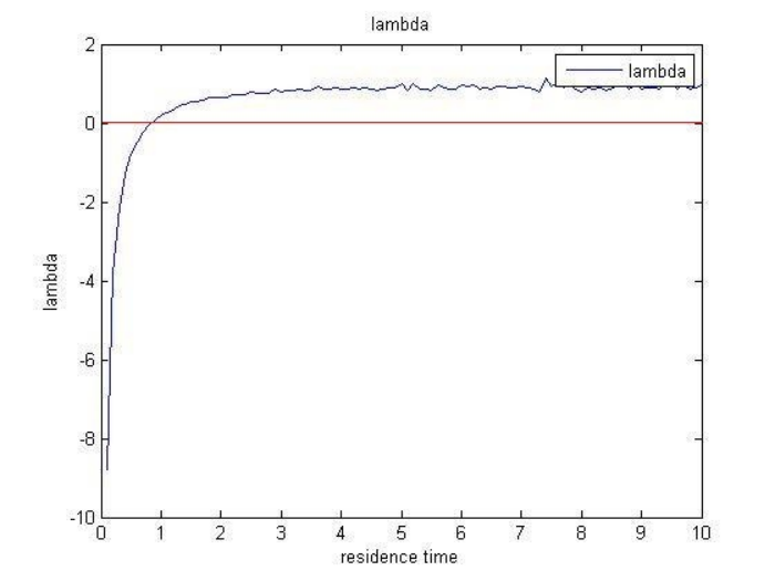
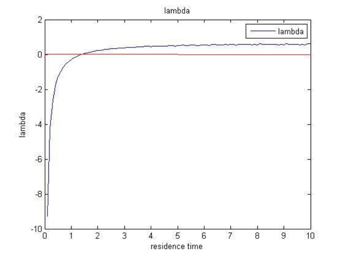
When one designs the treatment, a crucial design parameter is the so-called wash-out time. If the residence time $\theta$ is less than a critical value, denoted by $\theta_{0}$ , then the sewage flow is too fast for bacteria to grow, existing cells are flushed out faster than they can multiply. As a result, the bacteria become extinct. Figures 7 and 8 show that $\lambda$ is an increasing function of $\theta$ . By our theoretical results, to find the wash-out time $\theta_{0}$ , we need to solve the equation $\lambda(\theta)=0$ . For the system without switching (1.2), the value $\lambda$ can be obtained in a closed form by solving the Fokker-Planck equation. Then we can solve the equation $\lambda(\theta)=0$ by a standard numerical scheme. In Figure 8, we can see that $\theta_{0}\approx 1.4$ . When random switching are involved, the value of $\lambda$ in (2.4) cannot be solved in a closed form. However, because of the exponential convergence rate, one can also perform a numerical approximation to find $\theta_{0}$ . In Figure 7, $\theta_{0}\approx 0.8$ .

4 Controlled Stochastic Chemostat Models

To better help us reaching our goal of dynamically regulating and optimizing the performance of chemostat models, we introduce a control process in this section and consider controlled stochastic chemostat models. Note that for notational simplicity, we consider only the controlled dynamic systems without switching in this section. Switching can be added, but the notation would be much more complex. One needs to deal with a system of dynamic programming equations (partial differential equations) in lieu of a single equation. It seems to be more instructive to treat relatively simpler models to present the main ideas and leaving out the notational details.

Suppose that we can add a certain amount of bacteria $u(t)$ (the control) to the system at any time $t$ , which enables us to better adjust the system performance so as to minimize the amount of substrate over a long-time horizon. In this section, we focus on the case $f_{0}(s,i)=s$ . Then we have a controlled differential equation as follow

\begin{cases}\begin{aligned} dS(t)=&\left(\dfrac{S_{0}-S(t)}{\theta}-X(t)f_{1}(S(t),X(t))\right)dt+\sigma_{1}S(t)dW_{1}(t),\\ dX(t)=&\left(u(t)+X(t)\left(f_{2}(S(t),X(t))-k_{d}-\dfrac{1+R}{\theta}\right)\right)dt+\sigma_{2}X(t)dW_{2}(t).\end{aligned}\end{cases}

(4.1)

We assume the control $u(t)$ taking value in a compact interval $[0,M]$ for some $M>0$ . Our objective is to minimize

\limsup_{T\to\infty}\dfrac{1}{T}\mathbb{E}_{s,x}^{u}\int_{0}^{T}S(t)dt,

over the class of admissible controls $u(t)$ , where $u(t)$ is $\mathcal{F}_{t}$ -adapted. That is, we aim to minimize the amount of substrate over the infinite horizon. The cost criterion is in the sense of an average cost per unit time (or long-run average cost).

Before proceeding further, let us describe how we plan to carry out the analysis. In getting the desired optimal control, we need to obtain the Hamilton-Jacobi-Bellman (HJB) equation. We use a “vanishing discount argument”, which utilizes some ideas from the book [2]. Nevertheless, in the book, the HJB equation is derived under either “near-monotone” or “stable” conditions. Unfortunately, our model satisfies neither of these conditions. As a result, some new approaches are needed to obtain the HJB equation. The intuitive idea is to look at two different domains. In each of the domains, one of the “near-monotone” condition or the “stable” condition is satisfied. Nevertheless, the complication is that we also need to analyze the dynamics of the system, to investigate how the solution moves from one domain to the other, and to examine how the movement affects the objective function.

To proceed, we provide a road map of our approach. First, we recall some notation. Then the analysis is carried out using relaxed control setup and appropriate occupation measures. Theorem 4.2 presents the main result. To prove it, we need a number of technical results to take care of the situation as mentioned in the last paragraph regarding the two regions satisfying the “near-monotone” condition or “stable” conditions separately and the dynamic movements between these regions. These technical details are presented in a number of lemmas.

To continue, we recall some concepts and notation introduced in [2, 23]. Let $M(\infty)$ denote the family of measures $\{m(\cdot)\}$ on the Borel subsets of $[0,\infty)\times[0,M]$ satisfying $m([0,t]\times[0,M])=t$ for all $t\geq 0$ . By the weak convergence $m_{n}(\cdot)\rightarrow m(\cdot)$ in $M(\infty)$ , we mean $\lim_{n\to\infty}\int f(s,\alpha)m_{n}(ds\times d\alpha)=\int f(s,\alpha)m(ds\times d\alpha)$ for any continuous function $f(\cdot):[0,\infty)\times[0,M]\mapsto\mathbb{R}$ with compact support. A random measure $m(\cdot)$ with values in $M(\infty)$ is said to be an admissible relaxed control for (4.1) if $\int_{0}^{M}\int_{0}^{t}f(s,u)m(ds\times du)$ is independent of $\{W_{i}(t+s)-W_{i}(t),s>0,i=1,2\}$ for each bounded and continuous function $f(\cdot)$ . Under a relaxed control $m(\cdot)$ , the controlled diffusion (4.1) becomes

\begin{cases}\begin{aligned} dS(t)=&\left(\dfrac{S_{0}-S(t)}{\theta}-X(t)f_{1}\big(S(t),X(t)\big)\right)dt+\sigma_{1}S(t)dW_{1}(t),\\ dX(t)=&\left(\overline{m}_{t}+X(t)\left(f_{2}\big(S(t),X(t)\big)-\widetilde{k}_{d}\right)\right)dt+\sigma_{2}X(t)dW_{2}(t),\end{aligned}\end{cases}

(4.2)

where $\overline{m}_{t}=\int_{0}^{M}um_{t}(du)$ and the “derivative” $m_{t}$ is defined as the measure-valued function of $(\omega,t)$ such that for any smooth and bounded function $f$ , we have $\iint f(s,u)m(ds\times du)=\int ds\int f(s,u)m_{s}(du)$ . The operator associated with the controlled diffusion process (4.2), in which $t$ -dependence is hidden, is given by

	$\displaystyle{\cal L}^{m}\phi(s,x)=$	$\displaystyle\dfrac{\partial\phi(s,x)}{\partial s}\left[\frac{S_{0}-s}{\theta}-xf_{1}(s,x)\right]+\dfrac{\partial\phi(s,x)}{\partial x}\left[\overline{m}_{t}+xf_{2}(s,x)-x\widetilde{k}_{d}\right]$
		$\displaystyle+\dfrac{1}{2}\left(\sigma_{1}^{2}\dfrac{\partial^{2}\phi(s,x)}{\partial s^{2}}s^{2}+\sigma_{2}^{2}\dfrac{\partial^{2}\phi(s,x)}{\partial x^{2}}x^{2}\right).$

Definition 4.1.

We have the following definitions and notations.

•

Let $\mathcal{P}(M(\infty))$ be the space of probability measures on $M(\infty)$ . A relaxed control $m(\cdot)$ for (4.2) is said to be Markov if there exists a measurable function $v:\mathbb{R}^{2}_{+}\mapsto\mathcal{P}(M(\infty))$ such that $m_{t}=v(S(t),X(t)),t\geq 0.$ Under a relaxed Markov control $m_{t}=v(S(t),X(t))$ , the solution process $(S(t),X(t))$ to (4.2) is a Markov process with generator

	$\displaystyle{\cal L}^{v}\phi(s,x)=$	$\displaystyle\dfrac{\partial\phi(s,x)}{\partial s}\left[\frac{S_{0}-s}{\theta}-xf_{1}(s,x)\right]+\dfrac{\partial\phi(s,x)}{\partial x}\left[v(s,x)+xf_{2}(s,x)-x\widetilde{k}_{d}\right]$
		$\displaystyle+\dfrac{1}{2}\left(\sigma_{1}^{2}\dfrac{\partial^{2}\phi(s,x)}{\partial s^{2}}s^{2}+\sigma_{2}^{2}\dfrac{\partial^{2}\phi(s,x)}{\partial x^{2}}x^{2}\right).$

•

A Markov control $v$ is a relaxed control satisfying that $v(z)$ is a Dirac measure on $[0,M]$ for each $z\in\mathbb{R}^{2}_{+}$ .
•

Denote the set of Markov controls and relaxed Markov controls by $\Pi_{M}$ an $\Pi_{RM}$ , respectively. With a relaxed Markov control, $(S(t),X(t))$ is a Markov process that has the strong Feller property in $\mathbb{R}^{2,\circ}_{+}$ ; see [2, Theorem 2.2.12].
•

Since the diffusion is nondegenerate in $\mathbb{R}^{2,\circ}_{+}$ , if the process $(S(t),X(t))$ has an invariant probability measure in $\mathbb{R}^{2,\circ}_{+}$ , the invariant measure is unique, denoted by $\eta_{v}$ . In this case, the control $v$ is said to be stable. Denote by $\Pi_{SRM}$ the set of stable relaxed Markov controls.

•

Let $\mathcal{P}(\mathcal{X})$ be the space of probability measures on a metric space $\mathcal{X}$ . For any stable relaxed Markov control $v$ , define

\pi_{v}(dz\times du)=[v(z)(du)]\times\eta_{v}(du)\in\mathcal{P}(\mathbb{R}^{2,\circ}_{+}\times[0,M]),

and

\mathcal{G}=\{\pi_{v}:v\text{ is a stable relaxed Markov control }\}\subset\mathcal{P}(\mathbb{R}^{2,\circ}_{+}\times[0,M]).

We need the following lemma whose proof is analogous to [9, Lemma 2.3].

Lemma 4.1.

There exist a sufficiently small $p>0$ and positive constants $K_{1}$ , $K_{2}$ , and $K_{3}$ such that

{\cal L}^{m}(2\kappa_{0}s+x)\leq K_{1}-K_{2}(2\kappa_{0}s+x),

(4.3)

{\cal L}^{m}(2\kappa_{0}s+x)^{1+p}\leq K_{1}-K_{2}(2\kappa_{0}s+x)^{1+p}-K_{2}(2\kappa_{0}s+x)^{p}xf_{1}(s,x),

(4.4)

and

{\cal L}^{m}(2\kappa_{0}s+x)^{4}\leq K_{3}(1+2\kappa_{0}s+x)^{4},

(4.5)

for any admissible relax control $m(\cdot)$ . Consequently, it holds for any admissible relaxed control $m(\cdot)$ that

\mathbb{E}_{s,x}^{m}\big(2\kappa_{0}S(t)+X(t)\big)^{1+p}\leq(2\kappa_{0}s+x)^{1+p}e^{-K_{2}t}+\frac{K_{2}}{K_{1}}\text{ for }s>0,x\geq 0,

(4.6)

\mathbb{E}^{m}_{s,x}\int_{0}^{T}\big(2\kappa_{0}S(t)+X(t)\big)^{p}X(t)f_{1}(S(t),X(t))dt\leq(2\kappa_{0}s+x)^{1+p}+K_{1}T,

(4.7)

and

\mathbb{E}_{s,x}^{m}\big(2\kappa_{0}S(t)+X(t)\big)^{4}\leq(1+2\kappa_{0}s+x)^{4}e^{K_{3}t}\text{ for }s>0,x\geq 0,t\geq 0.

(4.8)

As a result, we have

\begin{array}[]{ll}&\!\!\!\displaystyle\int_{\mathbb{R}^{2,\circ}_{+}}(2\kappa_{0}s+x)^{1+p}\eta_{v}(ds,dx)\leq\frac{K_{2}}{K_{1}}\text{ and }\\ &\!\!\!\displaystyle\int_{\mathbb{R}^{2,\circ}_{+}}(2\kappa_{0}s+x)^{p}xf_{1}(s,x)\eta_{v}(ds,dx)\leq\frac{K_{2}}{K_{1}}\,\text{ for all }v\in\Pi_{RM}.\end{array}

(4.9)

Define the following sets

\mathcal{H}_{0}:=\left\{(s,x)\in\mathbb{R}^{2,\circ}_{+}:2\kappa_{0}s+x\leq\frac{K_{1}+1}{K_{2}}+2\kappa_{0}:=K_{4}\right\},

(4.10)

and

\mathcal{H}=\left\{(s,x)\in\mathbb{R}^{2,\circ}_{+}:2\kappa_{0}s+x\leq K_{4}\text{ and }s\geq\delta_{0}\right\}\subset\mathcal{H}_{0},

where $\delta_{0}$ is a positive constant to be determined in the proof of Lemma 4.2. For a closed set $\mathcal{K}\in\mathbb{R}^{2,\circ}_{+},$ define $\tau_{\mathcal{K}}=\inf\{t\geq 0:(S(t),X(t))\in\mathcal{K}\}$ . Since ${\cal L}^{u}(2\kappa_{0}s+x)\leq-1$ for $(s,x)\notin\mathcal{H}_{0},u\in[0,M]$ , we have

\mathbb{E}^{m}_{s,x}\tau_{\mathcal{H}_{0}}\leq 2\kappa_{0}s+x\,\text{ for any admissible relaxed control }\,m(t).

(4.11)

We have the following lemmas whose proofs are given in the appendix.

Lemma 4.2.

There is a constant $C_{1}>0$ depending only on $\mathcal{H}$ and $\mathcal{H}_{0}$ such that

\mathbb{E}^{v}_{s,x}\tau_{\mathcal{H}}\leq C_{1}\,\text{ for }\,(s,x)\in\mathcal{H}_{0},v\in\Pi_{RM}.

Moreover,

\mathbb{E}^{v}_{s,x}\tau_{\mathcal{H}}\leq 2\kappa_{0}s+x+C_{1},(s,x)\in\mathbb{R}^{2,\circ}_{+},v\in\Pi_{RM}.

(4.12)

With the constant control $v_{c}\equiv M$ , we have

\mathbb{E}^{v_{c}}_{s,x}\tau_{\mathcal{H}_{*}}\leq 2\kappa_{0}s+x+\widehat{C}_{1},(s,x)\in\mathbb{R}^{2,\circ}_{+},

(4.13)

where $\mathcal{H}_{*}$ is a compact subset of $\mathcal{H}_{0}$ , and $\widehat{C}_{1}$ is a positive constant depending on $\mathcal{H}_{0}$ and $\mathcal{H}_{*}$ .

Lemma 4.3.

For any $L_{1}>0$ and $\varepsilon>0$ , there exists a $\delta>0$ such that

\mathbb{P}_{s,\varepsilon}^{v}\{X(\tau_{\mathcal{H}})\geq\delta\}\geq\dfrac{1}{2},\text{ for any }s\leq L_{1},v\in\Pi_{RM}.

(4.14)

With these lemmas, let

\rho_{v}:=\int_{\mathbb{R}^{2,\circ}_{+}\times[0,M]}s\pi_{v}(ds\times dx\times du)\text{ and }\rho^{*}=\inf_{v\in\Pi_{SRM}}\left\{\rho_{v}\right\}.

Since (4.13) implies the existence of an invariant probability measure for $(S(t),X(t))$ under control $v_{c}$ , we claim that $\Pi_{SRM}\neq\emptyset$ . Moreover, for any admissible relaxed control $m(t)$ , we have that

\dfrac{\mathbb{E}_{s,x}^{m}S(T)-S(0)}{T}=\mathbb{E}_{s,x}^{m}\dfrac{1}{T}\int_{0}^{T}\left(\dfrac{S_{0}-S(t)}{\theta}-X(t)f_{1}\big(S(t),X(t)\big)\right)dt.

In view of (4.6), we have

\lim_{T\to\infty}\mathbb{E}_{s,x}^{m}\dfrac{1}{T}\int_{0}^{T}\left(\dfrac{S_{0}-S(t)}{\theta}-X(t)f_{1}\big(S(t),X(t)\big)\right)dt=\liminf_{T\to\infty}\dfrac{\mathbb{E}_{s,x}^{m}S(T)-S(0)}{T}=0,

(4.15)

which leads to

\int_{\mathbb{R}^{2,\circ}_{+}}\left(\dfrac{S_{0}-s^{\prime}}{\theta}-x^{\prime}f_{1}(s^{\prime},x^{\prime})\right)\eta_{v}(ds^{\prime},dx^{\prime})=0\,\text{ for any }\,v\in\Pi_{SRM}.

(4.16)

As a result,

$\displaystyle\rho^{*}\leq\lim_{T\to\infty}\mathbb{E}_{s,x}^{v_{c}}\dfrac{1}{T}\int_{0}^{T}S(t)dt=$	$\displaystyle\int_{\mathbb{R}^{2,\circ}_{+}}s^{\prime}\eta_{v_{c}}(ds^{\prime},dx^{\prime})$	(4.17)
$\displaystyle=$	$\displaystyle\theta\left[\dfrac{S_{0}}{\theta}-\int_{\mathbb{R}^{2,\circ}_{+}}x^{\prime}f_{1}(s^{\prime},x^{\prime})\eta_{v_{c}}(ds^{\prime},dx^{\prime})\right]$
$\displaystyle<$	$\displaystyle S_{0}.$

To proceed, we derive a lemma, which allows us to find an optimal control in $\Pi_{SRM}$ .

Lemma 4.4.

For any admissible relaxed control $m$ , define an empirical measure $\zeta_{T}^{m}$ as a $\mathcal{P}(\mathbb{R}^{2,\circ}_{+}\times[0,M])$ -valued process satisfying that

\int_{\mathbb{R}^{2,\circ}_{+}\times[0,M]}fd\zeta_{T}^{m}=\mathbb{E}^{m}_{s,x}\frac{1}{T}\int_{0}^{T}\left(\int_{0}^{M}f(S_{t},X_{t},u)m_{t}(du)\right)dt.

Then, with probability 1, every limit point of $\zeta_{T}^{m}$ as $T\to\infty$ can be decomposed as

\widehat{\zeta}=\delta\zeta^{\prime}+(1-\delta)\zeta^{\prime\prime},

(4.18)

where $\zeta^{\prime}\in\mathcal{G}$ and $\zeta^{\prime\prime}\in\mathcal{P}((0,\infty)\times\{0\}\times[0,M])$ satisfying

\int_{(0,\infty)\times\{0\}\times[0,M]}s\zeta^{\prime\prime}(ds,dx,du)=S_{0}.

As a result, for any admissible relaxed control $m$ ,

\liminf_{T\to\infty}\dfrac{1}{T}\mathbb{E}_{s,x}^{m}\int_{0}^{T}S(t)dt\geq\rho^{*}.

(4.19)

Lemma 4.4 enables us to find an optimal control that is a Markov relaxed control. To find the Markov control, we need to establish the HJB equation associated to the control problem (4.2). Let $\mathcal{C}_{1+p}$ be the class of functions $V:\mathbb{R}^{2,\circ}_{+}\mapsto\mathbb{R}$ such that $V(s,x)\leq c_{V}(1+s+x)^{1+p^{\prime}},(s,x)\in\mathbb{R}^{2,\circ}_{+}$ for some constants $c_{V}>0$ and $p^{\prime}\in(0,p)$ . The rest of this section aims to prove a theorem on the existence and uniqueness of solutions to the HJB equation.

Theorem 4.2.

There is a unique pair $(V,\rho)$ , where $V\in C^{2}(\mathbb{R}^{2,\circ}_{+})\cap\mathcal{C}_{1+p}$ and $\rho\in\mathbb{R}$ satisfying the equation

\min_{u\in[0,M]}\left\{{\cal L}^{u}V(s,x)+s\right\}=\rho.

Moreover, we have $\rho=\rho^{*}$ and $v^{*}\in\Pi_{RM}$ is an optimal control if and only if it is a measurable selector from the minimizer

\min_{u\in[0,M]}\left\{{\cal L}^{u}V(s,x)+s\right\}.

In fact, we can choose

v^{*}(s,x)=\begin{cases}0&\,\text{ if }\,\dfrac{\partial V(s,x)}{\partial x}\geq 0,\\ M&\,\text{ otherwise. }\end{cases}

In [2], the HJB equation is obtained under either of the following two assumptions: (a) the cost function satisfies the so-called near-monotone condition, or (b) any relax Markov control is stable and the set $\{\eta_{v},v\in\Pi_{RM}\}$ is tight. However, neither of these conditions are satisfied for our system. Thus the results in [2] are not directly applicable.

To prove the existence and uniqueness of solutions to the HJB equation, we use an idea that might be called a vanishing discount argument. That is, we examine the cost and value functions of the corresponding discounted control problem and look at the limit when the discount factor tends to $0.$ We also need to estimate the value function in different parts of $\mathbb{R}^{2,\circ}_{+}$ to obtain desired properties of the value functions, which is key to prove Theorem 4.2. That is the most difficult task of this section.

Let $V_{\gamma}(s,x)$ be the optimal $\gamma$ -discounted cost, that is

V_{\gamma}(s,x)=\inf\left\{\mathbb{E}^{m}_{s,x}\int_{0}^{\infty}e^{-\gamma t}S(t):m\text{ runs over the set of relaxed controls }\right\},\,(s,x)\in\mathbb{R}^{2,\circ}_{+}.

Then it follows from [2, Theorem 3.5.6 & Remark 3.5.8] that $V_{\gamma}(s,x)\in C^{2}(\mathbb{R}^{2,\circ}_{+})\cup C_{b}(\mathbb{R}^{2,\circ}_{+})$ satisfies

\min_{u\in[0,M]}\left\{{\cal L}^{u}V_{\gamma}(s,x)+s\right\}=\gamma V_{\gamma}(s,x).

(4.20)

and the optimal Markov control $v_{\gamma}$ is a selector of $\min_{u\in[0,M]}\left\{{\cal L}^{u}V_{\gamma}(s,x)+s\right\}$ . The following lemma is from [2, Lemma 3.7.8].

Lemma 4.5.

Fix $(s_{*},x_{*})\in\mathbb{R}^{2,\circ}_{+}$ . For any sequence $\gamma_{n}\downarrow 0$ , there exists a subsequence, which is still denoted by $\{\gamma_{n}\}$ , and a function $V\in C(\mathbb{R}^{2,\circ}_{+})$ and a constant $\rho$ such that as $n\to\infty$ , we have

\gamma_{n}V_{\gamma_{n}}(s_{*},x_{*})\to\rho\,\text{ and }\,\overline{V}_{\gamma_{n}}(s,x):=V_{\gamma_{n}}(s,x)-V_{\gamma_{n}}(s_{*},x_{*})\to V(s,x)

(4.21)

uniformly on each compact subset of $\mathbb{R}^{2,\circ}_{+}$ . Moreover, we have

\min_{u\in[0,M]}\left\{{\cal L}^{u}V(s,x)+s\right\}=\rho\leq\rho^{*},\,(s,x)\in\mathbb{R}^{2,\circ}_{+}.

We aim to show that a limit function $V$ in Lemma 4.5 belongs to the family $\mathcal{C}_{1+p}$ .

Proposition 4.1.

Let $V$ be any limit in (4.21). Then

\sup_{(s,x)\in\mathcal{H}}|V(s,x)|<\infty.

Proof.

Denoted by $v_{\gamma}$ the optimal Markov control of the $\gamma$ -discounted control problem. Let $\varepsilon_{*}=\frac{S_{0}-\rho^{*}}{5}$ , and $\overline{\rho}=\rho^{*}+\varepsilon_{*}=S_{0}-4\varepsilon^{*}$ and $C_{1}$ be as in Lemma 4.2. By (4.6), there exists a $C_{2}>0$ depending only on $\mathcal{H}_{0}$ such that

\mathbb{E}^{v_{\gamma}}_{s,x}(2\kappa_{0}S(t)+X(t))\leq C_{2},\text{ for any }(s,x)\in\mathcal{H}_{0},v\in\Pi_{RM},t\geq 0.

(4.22)

By Itô’s formula, we have that

\mathbb{E}^{v_{\gamma}}_{s,x}\left[S(t+h)-S(t)\right]=\int_{t}^{t+h}\left[\dfrac{S_{0}-\mathbb{E}^{v_{\gamma}}_{s,x}S(y)}{\theta}-\mathbb{E}^{v_{\gamma}}_{s,x}X(y)f_{1}\big(S(y),X(y)\big)\right]dy.

Letting $h\to 0$ , we obtain

\displaystyle\dfrac{d}{dt}\mathbb{E}^{v_{\gamma}}_{s,x}S(t)=

\displaystyle\dfrac{S_{0}-\mathbb{E}^{v_{\gamma}}_{s,x}S(t)}{\theta}-\mathbb{E}^{v_{\gamma}}_{s,x}X(t)f_{1}\big(S(t),X(t)\big).

(4.23)

Consider the differential equation

dz(t)=\frac{S_{0}-\varepsilon_{*}-z}{\theta}dt.

(4.24)

It is easy to show that $z(t)$ converges to $S_{0}-\varepsilon_{*}$ uniformly for each initial value belonging to any bounded set. Thus, there is a $T^{*}>\frac{\overline{\rho}(C_{1}+C_{2})+1}{\varepsilon_{*}}$ such that

\int_{0}^{T^{*}}z(t)dt\geq(S_{0}-2\varepsilon_{*})T^{*},\text{ for any }z(0)\geq 0.

(4.25)

In view of (4.21), we can choose $\gamma_{*}$ sufficiently small such that

(1-e^{-\gamma_{*}T^{*}})C_{2}\leq\varepsilon_{*},

(4.26)

and

\gamma V_{\gamma}(s_{*},x_{*})\leq\overline{\rho},\,\text{ for }\,\gamma<\gamma_{*}.

(4.27)

We divide $\mathcal{H}$ into two subsets (one of which can be empty):

\mathcal{H}^{\gamma}_{1}=\left\{(s,x)\in\mathcal{H}:\mathbb{E}^{v_{\gamma}}_{s,x}X(t)f_{1}\big(S(t),X(t)\big)\leq\frac{\varepsilon_{*}}{\theta},\text{ for all }t\in[0,T^{*}]\right\}\,\text{ and }\,\mathcal{H}^{\gamma}_{2}=\mathcal{H}\setminus\mathcal{H}^{\gamma}_{1}.

Step 1: Consider $(s,x)\in\mathcal{H}^{\gamma}_{1}$ . It follows from (4.23), (4.25), and a comparison argument of differential inequalities that

\mathbb{E}_{s,x}^{v_{\gamma}}\int_{0}^{T^{*}}S(t)dt\geq(S_{0}-2\varepsilon_{*})T^{*},(s,x)\in\mathcal{H}_{1}^{\gamma}.

(4.28)

Then, we derive from (4.22) and (4.26) that

\mathbb{E}_{s,x}^{v_{\gamma}}\int_{0}^{T^{*}}(1-e^{-\gamma t})S(t)dt\leq\varepsilon_{*}T^{*},\,(s,x)\in\mathcal{H}^{\gamma}_{1},\gamma<\gamma_{*}.

(4.29)

As a result of (4.28) and (4.29)

\mathbb{E}_{s,x}^{v_{\gamma}}\int_{0}^{T^{*}}e^{-\gamma t}S(t)dt\geq(S_{0}-3\varepsilon_{*})T^{*},\,\text{ for }\,(s,x)\in\mathcal{H}^{\gamma}_{1},\gamma<\gamma_{*}.

(4.30)

In view of (4.27), we have that

0\leq\inf_{(s,x)\in\mathcal{H}}V_{\gamma}(s,x)\leq\dfrac{\overline{\rho}}{\gamma}<\infty\,\text{ for }\,\gamma\leq\gamma_{*},

which combined with the strong Markov property of $(S(t),X(t))$ under a Markov control, implies

$\displaystyle V_{\gamma}(s,x)=$	$\displaystyle\mathbb{E}_{s,x}^{v_{\gamma}}\int_{0}^{\tau^{T^{}}_{\mathcal{H}}}e^{-\gamma t}S(t)dt+\mathbb{E}_{s,x}^{v_{\gamma}}\left[e^{-\gamma\tau^{T^{}}_{\mathcal{H}}}V_{\gamma}\left(S(\tau^{T^{}}_{\mathcal{H}}),X(\tau^{T^{}}_{\mathcal{H}})\right)\right]$	(4.31)
$\displaystyle\geq$	$\displaystyle\mathbb{E}_{s,x}^{v_{\gamma}}\int_{0}^{\tau^{T^{}}_{\mathcal{H}}}e^{-\gamma t}S(t)dt+\left(\inf_{(s,x)\in\mathcal{H}}V_{\gamma}(s,x)\right)\mathbb{E}_{s,x}^{v_{\gamma}}e^{-\gamma\tau^{T^{}}_{\mathcal{H}}}$
$\displaystyle\geq$	$\displaystyle\mathbb{E}_{s,x}^{v_{\gamma}}\int_{0}^{\tau^{T^{}}_{\mathcal{H}}}e^{-\gamma t}S(t)dt+\inf_{(s,x)\in\mathcal{H}}V_{\gamma}(s,x)-\dfrac{\overline{\rho}}{\gamma}\mathbb{E}_{s,x}^{v_{\gamma}}(1-e^{-\gamma\tau^{T^{}}_{\mathcal{H}}})\,\text{ for }\,(s,x)\in\mathbb{R}^{2,\circ}_{+},$

where $\tau^{T^{*}}_{\mathcal{H}}=\inf\{t\geq T^{*}:(S(t),X(t))\in\mathcal{H}\}$ . By the Markov property of $(S(t),X(t))$ , (4.22), and (4.12), we have

	$\displaystyle\dfrac{1}{\gamma}\mathbb{E}^{v_{\gamma}}_{s,x}(1-e^{-\gamma\tau^{T^{*}}_{\mathcal{H}}})\leq$	$\displaystyle\mathbb{E}^{v_{\gamma}}_{s,x}\tau^{T^{}}_{\mathcal{H}}\leq T^{}+\mathbb{E}^{v_{\gamma}}_{s,x}(\tau^{T^{}}_{\mathcal{H}}-T^{})$
	$\displaystyle=$	$\displaystyle T^{}+\mathbb{E}^{v_{\gamma}}_{s,x}\mathbb{E}^{v_{\gamma}}_{S(T^{}),X(T^{*})}\tau_{\mathcal{H}}$
	$\displaystyle\leq$	$\displaystyle T^{*}+C_{1}+C_{2}.$

This together with (4.30) and (4.31) implies

	$\displaystyle V_{\gamma}(s,x)\geq$	$\displaystyle\inf_{(s,x)\in\mathcal{H}}V_{\gamma}(s,x)+(S_{0}-3\varepsilon_{})T^{}-\overline{\rho}(T^{*}+C_{1}+C_{2})$
	$\displaystyle\geq$	$\displaystyle\inf_{(s,x)\in\mathcal{H}}V_{\gamma}(s,x)+\varepsilon_{}T^{}-\overline{\rho}(C_{1}+C_{2})\,\text{ (since }\overline{\rho}=S_{0}-4\varepsilon_{*})$
	$\displaystyle>$	$\displaystyle\inf_{(s,x)\in\mathcal{H}}V_{\gamma}(s,x)+1\,\text{ (since }T^{}>\dfrac{\overline{\rho}(C_{1}+C_{2})+1}{\varepsilon_{}}),$

which leads to

\overline{V}_{\gamma}(s,x)\geq\inf_{(s,x)\in\mathcal{H}}\overline{V}_{\gamma}(s,x)+1,(s,x)\in\mathcal{H}^{\gamma}_{1},\gamma\leq\gamma_{*}.

As a result,

\inf_{(s,x)\in\mathcal{H}}\overline{V}_{\gamma}(s,x)=\inf_{(s,x)\in\mathcal{H}^{\gamma}_{2}}\overline{V}_{\gamma}(s,x)\,\text{ for }\gamma\leq\gamma_{*}.

(4.32)

Step 2: Consider $(s,x)\in\mathcal{H}_{2}^{\gamma}$ . In view of (4.8), there is a $C_{3}>0$ depending only on $\mathcal{H}$ and $T^{*}$ such that

\mathbb{E}^{v_{\gamma}}_{s,x}(S^{4}(t)+X^{4}(t))\leq C_{3},\text{ for any }t\in[0,T^{*}],(s,x)\in\mathcal{H},v\in\Pi_{RM}.

(4.33)

For $(s,x)\in\mathcal{H}_{2}^{\gamma}$ , there is a $t_{s,x}\in[0,T^{*}]$ such that $\mathbb{E}^{v_{\gamma}}_{s,x}X(t_{s,x})f_{1}(S(t_{s,x}),X(t_{s,x}))\geq\dfrac{\varepsilon_{*}}{\theta}$ . Since $f_{1}(s,x)\leq\kappa_{0}(s+1)$ ,

\left[\mathbb{E}^{v_{\gamma}}_{s,x}X(t_{s,x})f_{1}(S(t_{s,x}),X(t_{s,x}))\right]^{2}\leq\kappa_{0}^{2}\mathbb{E}^{v_{\gamma}}_{s,x}X^{2}(t_{s,x})\mathbb{E}^{v_{\gamma}}_{s,x}(S(t_{s,x})+1)^{2},

which together with (4.33) implies

\mathbb{E}^{v_{\gamma}}_{s,x}X^{2}(t_{s,x})\geq\widehat{\varepsilon}_{*},

for some $\widehat{\varepsilon}_{*}\in(0,\frac{1}{2})$ depending on $\varepsilon_{*}$ and $C_{3}$ . Then

\mathbb{E}^{v_{\gamma}}_{s,x}\left[\boldsymbol{1}_{\{X^{2}(t_{s,x})<\frac{\widehat{\varepsilon}_{*}}{2}\}}X^{2}(t_{s,x})\right]+\mathbb{E}^{v_{\gamma}}_{s,x}\left[\boldsymbol{1}_{\{X^{2}(t_{s,x})\geq\frac{\widehat{\varepsilon}_{*}}{2}\}}X^{2}(t_{s,x})\right]\geq\widehat{\varepsilon}_{*},

which leads to

\mathbb{E}^{v_{\gamma}}_{s,x}\left[\boldsymbol{1}_{\{X^{2}(t_{s,x})\geq\frac{\widehat{\varepsilon}_{*}}{2}\}}X^{2}(t_{s,x})\right]\geq\dfrac{\widehat{\varepsilon}_{*}}{2}.

By Hölder’s inequality and (4.33), we have

	$\displaystyle\left(\mathbb{E}^{v_{\gamma}}_{s,x}\left[\boldsymbol{1}_{\{X^{2}(t_{s,x})\geq\frac{\widehat{\varepsilon}_{*}}{2}\}}X^{2}(t_{s,x})\right]\right)^{2}\leq$	$\displaystyle\mathbb{P}^{v_{\gamma}}_{s,x}\left\{X^{2}(t_{s,x})\geq\frac{\widehat{\varepsilon}_{*}}{2}\right\}\left[\mathbb{E}^{v_{\gamma}}_{s,x}X^{4}(t_{s,x})\right]$
	$\displaystyle\leq$	$\displaystyle C_{3}\mathbb{P}^{v_{\gamma}}_{s,x}\left\{X^{2}(t_{s,x})\geq\dfrac{\widehat{\varepsilon}_{*}}{2}\right\}.$

Thus,

\mathbb{P}^{v_{\gamma}}_{s,x}\left\{X^{2}(t_{s,x})\geq\frac{\widehat{\varepsilon}_{*}}{2}\right\}\geq\dfrac{\widehat{\varepsilon}_{*}^{2}}{4C_{3}}=:4\overline{q},\,\text{ for }(s,x)\in\mathcal{H}_{2}^{\gamma},

which implies that

\mathbb{P}^{v_{\gamma}}_{s,x}\{\eta\leq T^{*}\}\geq 4\overline{q},\text{ for }\,(s,x)\in\mathcal{H}^{\gamma}_{2},

(4.34)

where

\eta=\inf\left\{t\geq 0:X^{2}(t)\geq\frac{\widehat{\varepsilon}_{*}}{2}\right\}.

On the other hand, we have from Itô’s formula that

$\displaystyle\mathbb{E}^{v_{\gamma}}_{s,x}S(\eta\wedge T^{*})=$	$\displaystyle s+\mathbb{E}^{v_{\gamma}}_{s,x}\int_{0}^{\eta\wedge T^{*}}\left[\dfrac{S_{0}-S(t)}{\theta}-X(t)f_{1}(S(t),X(t))\right]dt$	(4.35)
$\displaystyle\leq$	$\displaystyle s+\dfrac{S_{0}}{\theta}\mathbb{E}^{v_{\gamma}}_{s,x}(\eta\wedge T^{*})$
$\displaystyle\leq$	$\displaystyle K_{4}+\dfrac{S_{0}T^{*}}{\theta}:=H_{1}.$

Defining

\tau^{\eta}_{\mathcal{H}}=\inf\{t\geq\eta\wedge T^{*}:(S(t),X(t))\in\mathcal{H}\},

we have

$\displaystyle\mathbb{E}^{v_{\gamma}}_{s,x}\tau^{\eta}_{\mathcal{H}}=$	$\displaystyle\mathbb{E}^{v_{\gamma}}_{s,x}(\eta\wedge T^{})+\mathbb{E}^{v_{\gamma}}_{s,x}(\tau^{\eta}_{\mathcal{H}}-(\eta\wedge T^{}))$	(4.36)
$\displaystyle\leq$	$\displaystyle T^{}+\mathbb{E}^{v_{\gamma}}_{s,x}\left[\mathbb{E}_{S(\eta\wedge T^{}),X(\eta\wedge T^{*})}^{v_{\gamma}}\tau_{\mathcal{H}}\right]$
$\displaystyle\leq$	$\displaystyle T^{}+\mathbb{E}^{v_{\gamma}}_{s,x}\left[2\kappa_{0}S(\eta\wedge T^{})+X(\eta\wedge T^{*})+C_{2}\right]$
$\displaystyle\leq$	$\displaystyle T^{*}+2\kappa_{0}H_{1}+1+C_{2}.$

It follows from (4.34), (4.35), and Markov’s inequality that

\mathbb{P}^{v_{\gamma}}_{s,x}\left\{\eta\leq T^{*}\,\text{ and }S(\eta)\leq\frac{H_{1}}{2\overline{q}}\,\right\}\geq 2\overline{q},\text{ for }\,(s,x)\in\mathcal{H}^{\gamma}_{2}.

(4.37)

By Lemma 4.3, there exists a $\delta_{*}>0$ depending only on $\frac{H_{1}}{2\overline{q}}$ and $\widehat{\varepsilon}_{*}$ such that

\mathbb{P}_{s,x}^{v_{\gamma}}\{X(\tau_{\mathcal{H}})\geq\delta_{*}\}>\frac{1}{2},\text{ for }s\leq\frac{H_{1}}{2\overline{q}},x^{2}\geq\frac{\widehat{\varepsilon}_{*}}{2},\gamma\in(0,1).

(4.38)

We can choose $\delta_{*}<x_{*}$ and define $\mathcal{H}_{3}=\{(s,x)\in\mathcal{H}:x\geq\delta_{*}\}$ . Then $\mathcal{H}_{3}$ is a compact subset of $\mathbb{R}^{2,\circ}_{+}$ . We have from the strong Markov property of $(S(t),X(t))$ under Markov control $v_{\gamma}$ and from (4.37) and (4.38) that

$\displaystyle\mathbb{P}^{v_{\gamma}}_{s,x}\left\{(S(\tau^{\eta}_{\mathcal{H}}),X(\tau^{\eta}_{\mathcal{H}}))\in\mathcal{H}_{3}\right\}\geq$	$\displaystyle\mathbb{E}^{v_{\gamma}}_{s,x}\left[\boldsymbol{1}_{\left\{\eta\leq T^{*}\,\text{ and }S(\eta)\leq\frac{H_{1}}{2\overline{q}}\,\right\}}\boldsymbol{1}_{\{(S(\tau^{\eta}_{\mathcal{H}}),X(\tau^{\eta}_{\mathcal{H}}))\in\mathcal{H}_{3}\}}\right]$	(4.39)
$\displaystyle=$	$\displaystyle\mathbb{E}^{v_{\gamma}}_{s,x}\left[\boldsymbol{1}_{\left\{\eta\leq T^{}\,\text{ and }S(\eta)\leq\frac{H_{1}}{2\overline{q}}\,\right\}}\mathbb{E}^{v_{\gamma}}_{S(\eta),X(\eta)}\boldsymbol{1}_{\{X(\tau_{\mathcal{H}})\geq\delta_{}\}}\right]$
$\displaystyle\geq$	$\displaystyle\dfrac{1}{2}\mathbb{E}^{v_{\gamma}}_{s,x}\left[\boldsymbol{1}_{\left\{\eta\leq T^{*}\,\text{ and }S(\eta)\leq\frac{H_{1}}{2\overline{q}}\,\right\}}\right]$
$\displaystyle\geq$	$\displaystyle\overline{q}.$

With $A=\left\{(S(\tau^{\eta}_{\mathcal{H}}),X(\tau^{\eta}_{\mathcal{H}}))\in\mathcal{H}_{3}\right\}$ and $A^{c}=\Omega\setminus A$ , we have the estimate

	$\displaystyle\overline{V}_{\gamma}(s,x)=$	$\displaystyle\mathbb{E}^{v_{\gamma}}_{s,x}\int_{0}^{\tau^{\eta}_{\mathcal{H}}}e^{-\gamma t}S(t)dt+\mathbb{E}^{v_{\gamma}}_{s,x}\left[e^{-\gamma\tau^{\eta}_{\mathcal{H}}}V_{\gamma}\left(S(\tau^{\eta}_{\mathcal{H}}),X(\tau^{\eta}_{\mathcal{H}})\right)\right]-V_{\gamma}(s_{},x_{})$
	$\displaystyle\geq$	$\displaystyle\mathbb{E}^{v_{\gamma}}_{s,x}\left[\boldsymbol{1}_{A}e^{-\gamma\tau^{\eta}_{\mathcal{H}}}\inf_{(s^{\prime},x^{\prime})\in\mathcal{H}_{3}}V_{\gamma}(s^{\prime},x^{\prime})\right]+\mathbb{E}^{v_{\gamma}}_{s,x}\left[\boldsymbol{1}_{A^{c}}e^{-\gamma\tau^{\eta}_{\mathcal{H}}}\inf_{(s^{\prime},x^{\prime})\in\mathcal{H}}V_{\gamma}(s^{\prime},x^{\prime})\right]-V_{\gamma}(s_{},x_{})$
	$\displaystyle=$	$\displaystyle\mathbb{E}^{v_{\gamma}}_{s,x}\left[\boldsymbol{1}_{A}\left(\inf_{(s^{\prime},x^{\prime})\in\mathcal{H}_{3}}V_{\gamma}(s^{\prime},x^{\prime})-V_{\gamma}(s_{},x_{})\right)\right]$
		$\displaystyle+\mathbb{E}^{v_{\gamma}}_{s,x}\left[\boldsymbol{1}_{A^{c}}\left(\inf_{(s^{\prime},x^{\prime})\in\mathcal{H}}V_{\gamma}(s^{\prime},x^{\prime})-V_{\gamma}(s_{},x_{})\right)\right]$
		$\displaystyle-\mathbb{E}^{v_{\gamma}}_{s,x}\left[\boldsymbol{1}_{A}(1-e^{-\gamma\tau^{\eta}_{\mathcal{H}}})\inf_{(s^{\prime},x^{\prime})\in\mathcal{H}_{3}}V_{\gamma}(s^{\prime},x^{\prime})\right]$
		$\displaystyle-\mathbb{E}^{v_{\gamma}}_{s,x}\left[\boldsymbol{1}_{A^{c}}(1-e^{-\gamma\tau^{\eta}_{\mathcal{H}}})\inf_{(s^{\prime},x^{\prime})\in\mathcal{H}}V_{\gamma}(s^{\prime},x^{\prime})\right].$

Since $\overline{V}_{\gamma}(s,x)=V_{\gamma}(s,x)-V_{\gamma}(s_{*},x_{*})\to V(s,x)$ as $\gamma\to 0$ uniformly in each compact set, there exists an $H_{2}>0$ such that $|\overline{V}_{\gamma}(s,x)|<H_{2}$ for $(s,x)\in\mathcal{H}_{3}$ when $\gamma$ is sufficiently small. We also have $0\leq\inf_{(s^{\prime},x^{\prime})\in\mathcal{H}_{3}}V_{\gamma}(s^{\prime},x^{\prime})\leq V(s_{*},x_{*})\leq\frac{\overline{\rho}}{\gamma}$ when $\gamma$ is sufficiently small. This together with (4.36), (4.39), and $\inf_{(s,x)\in\mathcal{H}}\overline{V}_{\gamma}(s,x)\leq 0$ yields that

	$\displaystyle\overline{V}_{\gamma}(s,x)\geq$	$\displaystyle-H_{2}\mathbb{P}^{v_{\gamma}}_{s,x}(A)+\inf_{(s^{\prime},x^{\prime})\in\mathcal{H}}\overline{V}_{\gamma}(s^{\prime},x^{\prime})\mathbb{P}^{v_{\gamma}}_{s,x}(A^{c})-\overline{\rho}\mathbb{E}^{v_{\gamma}}_{s^{\prime},x^{\prime}}\left[\dfrac{1-e^{-\gamma\tau^{\eta}_{\mathcal{H}}}}{\gamma}\right]$
	$\displaystyle\geq$	$\displaystyle-H_{2}\mathbb{P}^{v_{\gamma}}_{s,x}(A)+\inf_{(s^{\prime},x^{\prime})\in\mathcal{H}}\overline{V}_{\gamma}(s^{\prime},x^{\prime})\mathbb{P}^{v_{\gamma}}_{s,x}(A^{c})-\overline{\rho}\mathbb{E}^{v_{\gamma}}_{s,x}\tau^{\eta}_{\mathcal{H}}$
	$\displaystyle\geq$	$\displaystyle-H_{2}-\overline{\rho}\left(T^{*}+2\kappa_{0}H_{1}+1+C_{2}\right)+\inf_{(s^{\prime},x^{\prime})\in\mathcal{H}}\overline{V}_{\gamma}(s^{\prime},x^{\prime})\mathbb{P}^{v_{\gamma}}_{s,x}(A^{c}),$
	$\displaystyle\geq$	$\displaystyle-H_{2}-\overline{\rho}\left(T^{*}+2\kappa_{0}H_{1}+1+C_{2}\right)+\inf_{(s^{\prime},x^{\prime})\in\mathcal{H}}\overline{V}_{\gamma}(s^{\prime},x^{\prime})(1-\overline{q}),\text{ for any }(s,x)\in\mathcal{H}_{2}^{\gamma},$

which combined with (4.32) leads to

\inf_{(s,x)\in\mathcal{H}}\overline{V}_{\gamma}(s,x)\geq-H_{2}-\overline{\rho}\left(T^{*}+2\kappa_{0}H_{1}+1+C_{2}\right)+\inf_{(s,x)\in\mathcal{H}}\overline{V}_{\gamma}(s,x)(1-\overline{q}),

\displaystyle\inf_{(s,x)\in\mathcal{H}}\overline{V}_{\gamma}(s,x)\geq

\displaystyle-\dfrac{1}{\overline{q}}\left(H_{2}+\overline{\rho}\left(T^{*}+2\kappa_{0}H_{1}+1+C_{2}\right)\right)=:-H_{3}.

(4.40)

Let $v_{c}\equiv M$ be the constant control. Similar to the proof of Lemma 4.2, we can show that

H_{4}:=\sup_{(s,x)\in\mathcal{H}}\mathbb{E}^{v_{c}}_{s,x}\tau_{\mathcal{H}_{3}}<\infty.

We have

\mathbb{E}^{v_{c}}_{s,x}S(\tau_{\mathcal{H}_{3}})\leq s+\dfrac{S_{0}}{\theta}\mathbb{E}^{v_{c}}_{s,x}\tau_{\mathcal{H}_{3}}-\frac{1}{\theta}\mathbb{E}^{v_{c}}_{s,x}\int_{0}^{\tau_{\mathcal{H}_{3}}}S(t),

which implies

\mathbb{E}^{v_{c}}_{s,x}\int_{0}^{\tau_{\mathcal{H}_{3}}}S(t)\leq\theta s+S_{0}\mathbb{E}^{v_{c}}_{s,x}\tau_{\mathcal{H}_{3}}\leq\theta K_{4}+S_{0}H_{4},(s,x)\in\mathcal{H}.

(4.41)

By [2, Eq. (3.7.47)],

	$\displaystyle V(s,x)\leq$	$\displaystyle\mathbb{E}^{v_{c}}_{s,x}\left[\int_{0}^{\tau_{\mathcal{H}_{3}}}S(t)dt+V(S(\tau_{\mathcal{H}_{3}}),X(\tau_{\mathcal{H}_{3}}))\right]$		(4.42)
	$\displaystyle\leq$	$\displaystyle\theta K_{4}+S_{0}H_{4}+\sup_{(s^{\prime},x^{\prime})\in\mathcal{H}_{3}}V(s^{\prime},x^{\prime}).$		(4.42)

From (4.40) and (4.42), we obtain that

\sup_{(s,x)\in\mathcal{H}}|V(s,x)|<\infty.

∎

Proof of Theorem 4.2.

For any $(s,x)\in\mathbb{R}^{2,\circ}_{+}$ , we have

$\displaystyle\overline{V}_{\gamma}(s,x)=$	$\displaystyle\mathbb{E}^{v_{\gamma}}_{s,x}\int_{0}^{\tau_{\mathcal{H}}}e^{-\gamma t}S(t)dt+\mathbb{E}^{v_{\gamma}}_{s,x}\left[e^{-\gamma\tau_{\mathcal{H}}}V_{\gamma}\left(S(\tau_{\mathcal{H}}),X(\tau^{T}_{\mathcal{H}})\right)\right]-V_{\gamma}(s_{},x_{})$	(4.43)
$\displaystyle\geq$	$\displaystyle\inf_{(s^{\prime},x^{\prime})\in\mathcal{H}}\overline{V}_{\gamma}(s^{\prime},x^{\prime})-\mathbb{E}^{v_{\gamma}}_{s,x}\frac{\rho}{\gamma}(1-e^{-\gamma\tau_{\mathcal{H}}})$
$\displaystyle\geq$	$\displaystyle\inf_{(s^{\prime},x^{\prime})\in\mathcal{H}}\overline{V}_{\gamma}(s^{\prime},x^{\prime})-\mathbb{E}^{v_{\gamma}}_{s,x}\tau_{\mathcal{H}}$
$\displaystyle\geq$	$\displaystyle-(H_{3}+2\kappa_{0}s+x+C_{1})\quad\text{due to \eqref{lm3.5-e17} and \eqref{lm3.3-e0}.}$

As a result,

V(s,x)\geq-(H_{3}+2\kappa_{0}s+x+C_{1}+1).

Similar to (4.41) and (4.42), we have

$\displaystyle V(s,x)\leq$	$\displaystyle\mathbb{E}^{v_{c}}_{s,x}\left[\int_{0}^{\tau_{\mathcal{H}}}S(t)dt+V(S(\tau_{\mathcal{H}}),X(\tau_{\mathcal{H}}))\right]$	(4.44)
$\displaystyle\leq$	$\displaystyle\sup_{(s^{\prime},x^{\prime})\in\mathcal{H}}\|V(s^{\prime},x^{\prime})\|+\theta s+S_{0}\mathbb{E}^{v_{c}}_{s,x}\tau_{\mathcal{H}}$
$\displaystyle\leq$	$\displaystyle\sup_{(s^{\prime},x^{\prime})\in\mathcal{H}}\|V(s^{\prime},x^{\prime})\|+\theta s+S_{0}(2\kappa_{0}s+x+\widehat{C}_{1}).$

In view of (4.43) and (4.44), we have $V(s,x)\in\mathcal{C}_{1+p}$ . Then, we can use arguments similar to [2, Theorem 3.7.11 and Theorem 3.7.12] and Lemma 4.4 to obtain the desired result. ∎

5 Concluding Remarks

To validate and to improve model (1.2), verification using real data is needed. To verify the model, the parameters of the system need to be estimated first. A statistical estimator can be constructed. To estimate the parameters using real data, we observe the solutions of (1.2) in discrete epoch, and carry out the estimation accordingly. That is, view the observation (the real data) as solution of (1.2), then use the explicit Euler method to discretize the diffusion process (1.2), and utilize for example, the maximum likelihood method to estimate the parameter. An alternative approach is to use the generalized method of moments.

The simplified model (1.2) may not be sufficient to perceive the complicated process of wastewater treatment. Considering more complex models renders better understanding but also poses more challenges.

In Section 4, we worked with controlled diffusions without switching for notational simplicity. The proofs carry over if one considers the controlled switching diffusion counterpart of (4.1). We have proved the existence and uniqueness of solutions to the HJB equation for (4.1). For the controlled switching diffusions, we need to deal with a system of HJB equations. While the optimal Markov control can be obtained theoretically using the system of HJB equations, it is quite difficult to find a closed-form solution explicitly. Constructing a numerical scheme is a viable alternative.

Appendix A Proofs of Theorem 2.1

Proof of Theorem 2.1.

Since the coefficients of (1.3) are locally Lipschitz continuous in $(s,x,i)\in\mathbb{R}_{+}^{2}\times\mathcal{M}$ , the system given by (1.3) and (1.4) has a unique continuous solution up to explosion time $\tau_{e}$ , where $\tau_{e}=\inf\{t\geq 0:S(t)\vee X(t)=\infty\}$ , with the convention $\inf\emptyset=\infty$ . The solution is also a strong Markov process; see [24, 42]. If we define

\tau_{k}=\inf\Big\{t\geq 0:S(t)\vee X(t)>k\Big\},

then $\tau_{e}=\lim_{k\to\infty}\tau_{k}$ . Consider $\widehat{V}_{1}(s,x,i)=\kappa_{0}s+x$ then, by the generalized Itô formula, we have

	$\displaystyle\mathcal{L}\widehat{V}_{1}(s,x,i)$	$\displaystyle=\dfrac{S_{0}\kappa_{0}}{\theta}-\dfrac{\kappa_{0}}{\theta}f_{0}(s,i)-\widetilde{k}_{d}(i)x+x(f_{2}(s,x,i)-\kappa_{0}f_{1}(s,x,i))$
		$\displaystyle\leq\dfrac{S_{0}\kappa_{0}}{\theta}.$

Hence,

\displaystyle\mathbb{E}_{s,x,i}\widehat{V}_{1}\big(S(\tau_{k}\wedge t),X(\tau_{k}\wedge t),\alpha(\tau_{k}\wedge t)\big)\leq\widehat{V}_{1}(s,x,i)+\dfrac{S_{0}\kappa_{0}t}{\theta},

which implies that

	$\displaystyle\mathbb{P}_{s,x,i}\big\{\tau_{k}<t\big\}$	$\displaystyle\leq\mathbb{P}_{s,x,i}\Big\{\widehat{V}_{1}\big(S(\tau_{k}\wedge t),X(\tau_{k}\wedge t),\alpha(\tau_{k}\wedge t)\big)\geq k\Big\}$
		$\displaystyle\leq\dfrac{\widehat{V}_{1}(s,x,i)+\frac{S_{0}\kappa_{0}t}{\theta}}{k}\to 0\;\text{as}\;k\to\infty.$

Therefore, we have $\mathbb{P}_{s,x,i}\{\tau_{e}\leq t\}=0$ or $\mathbb{P}_{s,x,i}\{\tau_{e}>t\}=1\;\forall t>0$ . As a consequence, $\mathbb{P}_{s,x,i}\{\tau_{e}=\infty\}=1$ . Hence, the system given by (1.3) and (1.4) has a unique global continuous solution.

Now, we move to the part of positivity of solutions. First, suppose that $s,x>0$ . For any $n\in{\mathbb{Z}}_{+}$ , we define the following truncated functions

f_{0}^{(n)}(s,i)=f_{0}(s\wedge n,i)\;;\;f_{1}^{(n)}(s,x,i)=f_{1}(s\wedge n,x\wedge n,i)\;;\;f_{2}^{(n)}(s,x,i)=f_{2}(s\wedge n,x\wedge n,i),

and let $\big(S^{(n)}(t),X^{(n)}(t)\big)$ be the solution of equation (1.3) and (1.4) with $f_{0},f_{1},f_{2}$ replaced by $f_{0}^{(n)},f_{1}^{(n)},f_{2}^{(n)}$ , respectively. Denote

\eta^{(n)}=\inf\big\{t\geq 0:S^{(n)}(t)\wedge X^{(n)}(t)\leq 0\big\},

\eta_{k}^{(n)}=\inf\Big\{t\geq 0:S^{(n)}(t)\wedge X^{(n)}(t)<\dfrac{1}{k}\Big\}.

Then $\eta^{(n)}=\lim_{k\to\infty}\eta_{k}^{(n)}$ . Consider

\widehat{V}_{2}^{(n)}(s,x,i)=s-c_{1}^{(n)}-c_{1}^{(n)}\ln\dfrac{s}{c_{1}^{(n)}}+c_{2}(x-1-\ln x),

where

c_{2}=\dfrac{1}{\kappa_{0}}\;\text{and}\;c_{1}^{(n)}=\frac{c_{2}\check{k}_{d}}{\max_{i\in\mathcal{M}}\sup_{s>0}\frac{f_{1}^{(n)}(s,x,i)}{s}}.

Let

c_{2}^{(n)}:=\max_{i\in\mathcal{M}}\sup_{s>0}\frac{f_{0}^{(n)}(s,i)}{s}.

Since $f_{1}^{(n)}(s,x,i)$ is global Lipschitz and $f_{1}^{(n)}(0,x,i)=0$ , it is readily seen that $\displaystyle\sup_{s>0}\frac{f_{1}^{(n)}(s,x,i)}{s}<\infty$ . Similarly, we also obtain $\sup_{s>0}\frac{f_{0}^{(n)}(s,i)}{s}<\infty$ , so the above constants are well-defined.

By the generalized Itô formula, we have

\begin{aligned} \mathcal{L}^{(n)}\widehat{V}_{2}^{(n)}(s,x,i)=&\Big(1-\dfrac{c_{1}^{(n)}}{s}\Big)\left(\dfrac{S_{0}}{\theta}-\dfrac{f_{0}^{(n)}(s,i)}{\theta}-xf_{1}^{(n)}(s,x,i)\right)+\dfrac{c_{1}^{(n)}\sigma_{1}^{2}(i)}{2}\\ &+\Big(c_{2}-\dfrac{c_{2}}{x}\Big)\left(xf_{2}^{(n)}(s,x,i)-x\widetilde{k}_{d}(i)\right)+\dfrac{c_{2}\sigma_{2}^{2}(i)}{2}\\ \leq&\dfrac{S_{0}+c_{1}^{(n)}c_{2}^{(n)}}{\theta}+c_{2}\widehat{k}_{d}+\dfrac{c_{1}^{(n)}\widehat{\sigma}_{1}^{2}+c_{2}\widehat{\sigma}_{2}^{2}}{2}\\ &+x\Big(c_{2}f_{2}^{(n)}(s,x,i)-f_{1}^{(n)}(s,x,i)\Big)+x\Big(\dfrac{c_{1}^{(n)}f_{1}^{(n)}(s,x,i)}{s}-c_{2}k_{d}(i)\Big)\\ \leq&\dfrac{S_{0}+c_{1}^{(n)}c_{2}^{(n)}}{\theta}+c_{2}\widehat{k}_{d}+\dfrac{c_{1}^{(n)}\widehat{\sigma}_{1}^{2}+c_{2}\widehat{\sigma}_{2}^{2}}{2}:=K^{(n)}\text{ for }s,x>0,\end{aligned},

where the operator $\mathcal{L}^{(n)}$ is defined as $\mathcal{L}$ with $f_{0}$ , $f_{1}$ , and $f_{2}$ replaced by $f_{0}^{(n)}$ , $f_{1}^{(n)}$ , and $f_{2}^{(n)}$ , respectively. Applying Itô’s formula again, we have

	$\displaystyle\mathbb{E}_{s,x,i}$	$\displaystyle\widehat{V}_{2}^{(n)}\big(S^{(n)}(\eta_{k}^{(n)}\wedge t),X^{(n)}(\eta_{k}^{(n)}\wedge t),\alpha(\eta_{k}^{(n)}\wedge t)\big)$
	$\displaystyle=$	$\displaystyle\widehat{V}_{2}^{(n)}(s,x,i)+\mathbb{E}_{s,x,i}\int_{0}^{\eta_{k}^{(n)}\wedge t}\mathcal{L}\widehat{V}_{2}^{(n)}\big(S^{(n)}(u),X^{(n)}(u),\alpha(u)\big)du$
	$\displaystyle\leq$	$\displaystyle\widehat{V}_{2}^{(n)}(s,x,i)+K^{(n)}t.$

Since the definition of $\widehat{V}_{2}^{(n)}$ , we observe that if $\eta_{k}^{(n)}<t$ , then

\widehat{V}_{2}^{(n)}\big(S^{(n)}(\eta_{k}^{(n)}\wedge t),X^{(n)}(\eta_{k}^{(n)}\wedge t),\alpha(\eta_{k}^{(n)}\wedge t)\big)\geq\big(c_{1}^{(n)}\ln kc_{1}^{(n)}-c_{1}^{(n)}\big)\wedge\big(c_{2}\ln k-c_{2}\big).

Hence, we obtain that

\displaystyle\mathbb{P}_{s,x,i}\{\eta_{k}^{(n)}<t\}\leq\dfrac{\widehat{V}_{2}^{(n)}(s,x,i)+K^{(n)}t}{\big(c_{1}^{(n)}\ln kc_{1}^{(n)}-c_{1}^{(n)}\big)\wedge\big(c_{2}\ln k-c_{2}\big)}\to 0\;\text{as}\;k\to\infty.

As a result, for any $n\in{\mathbb{Z}}_{+}$ , $\mathbb{P}_{s,x,i}\{\eta^{(n)}_{\infty}=\infty\}=1$ . That is,

\mathbb{P}_{s,x,i}\big\{S^{(n)}(t),X^{(n)}(t)>0:\forall t>0\big\}=1\text{ for any }n\in{\mathbb{Z}}_{+},

and hence

\mathbb{P}_{s,x,i}\big\{S^{(n)}(t),X^{(n)}(t)>0:\forall t>0,n\in{\mathbb{Z}}_{+}\big\}=1.

Now, for any $t>0$ and

\omega\in\{\tau_{e}=\infty\}\cap\big\{S^{(n)}(t),X^{(n)}(t)>0:\forall t>0,n\in{\mathbb{Z}}_{+}\big\},

there exists $n_{0}=n_{0}(\omega,t)$ such that

S(y)(\omega)\vee X(y)(\omega)<n_{0}\;\forall 0\leq y\leq t.

As a consequence, $S(t)(\omega)=S^{(n_{0})}(t)(\omega)>0$ and $X(t)(\omega)=X^{(n_{0})}(t)(\omega)>0$ . This, combined with $\mathbb{P}_{s,x,i}\{\tau_{e}=\infty\}=1$ , implies that

\mathbb{P}_{s,x,i}\big\{S(t)>0:t>0\big\}=\mathbb{P}_{s,x,i}\big\{X(t)>0:t>0\big\}=1\;\forall s,x>0.

(A.1)

If $s>0,x=0$ , the result $\mathbb{P}_{s,x,i}\big\{S(t)>0:t>0\big\}=1$ is similar proved by choosing $c_{2}=0$ . Moreover, it is obvious that $\mathbb{P}_{s,x,i}\big\{X(t)=0:t>0\big\}=1$ .

Consider the case when the initial value $s=0$ and $x\geq 0$ . Let $\varepsilon>0$ be sufficiently small such that

\dfrac{S_{0}-f_{0}(\tilde{s},i)}{\theta}-\tilde{x}f_{1}(\tilde{s},\tilde{x},i)\geq\frac{S_{0}}{2\theta},

(A.2)

for any $(\tilde{s},\tilde{x},\tilde{i})\in\mathbb{R}^{2}\times\mathcal{M}$ satisfying $\tilde{s}+|\tilde{x}-x|<\varepsilon$ . Let

\tilde{\tau}_{1}=\inf\{t>0:S(t)+|X(t)-x|\geq\varepsilon\}.

By the continuity of $(S(t),X(t))$ , $\mathbb{P}_{0,x,i}\{\tilde{\tau}_{1}>0\}=1$ . Using the variation of constants formula (see [24, Chapter 3]), we can write $S(t)$ in the form

\begin{array}[]{ll}&\!\!\!\displaystyle S(t)=\Phi(t)\left[\int_{0}^{t}\Phi^{-1}(u)\left(\dfrac{S_{0}-f_{0}\big(S(u),\alpha(u)\big)}{\theta}-X(u)f_{1}\big(S(u),X(u),\alpha(u)\big)\right)du\right]\\ &\displaystyle\ \hfill\text{ for }t\in[0,\tilde{\tau}_{1}),\end{array}

(A.3)

where $\Phi(t)=\exp\left(-\int_{0}^{t}\dfrac{\sigma_{1}^{2}(\alpha(u))}{2}du+\int_{0}^{t}\sigma_{1}(\alpha(u))dW_{2}(u)\right).$ It follows from (A.2) that

\frac{S_{0}-f_{0}\big(S(u),\alpha(u)\big)}{\theta}-X(u)f_{1}\big(S(u),X(u),\alpha(u)\big)>0\;\text{if}\;t\in(0,\tilde{\tau}_{1}].

This and (A.3) imply that

\mathbb{P}_{0,x,i}\{S(t)>0,t\in(0,\tilde{\tau}_{1}]\}=1,

which combined with (A.1) and the strong Markov property of $(S(t),X(t),\alpha(t))$ yields that

\mathbb{P}_{0,x,i}\{S(t)>0,t\in(0,\infty)\}=1.

The theorem is therefore proved. ∎

Appendix B Proof of Lemmas in Section 4

Proof of Lemma 4.2.

Since $f_{1}(0,x)=0$ , we can choose $\delta_{1}>0$ such that $s+\theta xf_{1}(s,x)\leq\frac{S_{0}}{2}$ for $s\leq\delta_{1},x\leq K_{4}$ , where $K_{4}$ is defined in (4.10). Due to the uniform bound from (4.3) and the stochastic continuity of $S(t)$ , (which can be seen to be uniform in $v$ since the equation of $S(t)$ does not depend directly on $v$ ), there exist $t_{1}\in(0,\frac{1}{2})$ and $\widehat{\delta}_{1}\in(0,\delta_{1})$ such that

\mathbb{P}^{v}_{s,x}\left\{S(t)<\delta_{1},X(t)\leq K_{4}+1,t\in[0,t_{1}]\right\}\geq\frac{3}{4},(s,x)\in\mathcal{H}_{0},s<\widehat{\delta}_{1}.

(B.1)

Let $K_{5}$ be sufficiently large such that

\mathbb{P}\left\{\Phi(t)\vee\Phi^{-1}(t)<K_{5},t\in[0,t_{1}]\right\}\geq\frac{3}{4},

(B.2)

where in this section, $\Phi(t)=\exp\left(-\frac{\sigma_{1}^{2}}{2}t+\int_{0}^{t}\sigma_{1}dW_{1}(u)\right).$ If $\Phi(t)\vee\Phi^{-1}(t)<K_{5}$ and $S(t)+\theta X(t)f_{1}(S(t),X(t))\leq\frac{S_{0}}{2}$ for $t\in[0,t_{1}]$ , we have

S(t_{1})=\Phi(t)\int_{0}^{t}\Phi^{-1}(t)\left(\frac{S(u)-S_{0}}{\theta}-X(u)f_{1}(S(u),X(u))\right)du\geq\frac{t_{1}S_{0}}{2\theta K_{5}^{2}}.

(B.3)

Let $\delta_{0}:=\frac{t_{1}S_{0}}{2\theta K_{5}^{2}}\wedge\widehat{\delta}_{1}$ and $\mathcal{H}=\{(s,x):2\kappa_{0}s+x\leq K_{4},s\geq\delta_{0}\}$ . Since the diffusion is nondegenerate on $\mathbb{R}^{2,\circ}_{+}$ , it is well-known (see e.g., [2, Lemma 2.6.5]) that there exist $t_{2}>0$ and $p_{1}>0$ such that

\mathbb{P}^{v}_{s,x}\left\{\tau_{\mathcal{H}}<t_{2}\right\}>2p_{1},\text{ provided }\delta_{0}\leq s\leq\delta_{1},K_{4}-2\kappa_{0}\delta_{1}\leq x\leq K_{4}+1.

Because of the definition of $\mathcal{H}$ ,

\mathbb{P}^{v}_{s,x}\left\{\tau_{\mathcal{H}}<t_{2}\right\}>2p_{1},\text{ provided }\delta_{0}\leq s\leq\delta_{1},x\leq K_{4}+1.

This together with (B.1), (B.2), (B.3), and the definition of $\delta_{0}$ implies

\mathbb{P}_{s,x}^{v}\left\{\tau_{\mathcal{H}}<t_{1}+t_{2}\right\}\geq p_{1},\,(s,x)\in\mathcal{H}_{0}.

(B.4)

Define stopping times

		$\displaystyle\tau^{(1)}_{\mathcal{H}_{0}}=\inf\{t\geq t_{1}+t_{2}:(S(t),X(t))\in\mathcal{H}_{0}\},$
		$\displaystyle\tau^{(n+1)}_{\mathcal{H}_{0}}=\inf\{t\geq\tau^{n}_{H}+t_{1}+t_{2}:(S(t),X(t))\in\mathcal{H}_{0}\}.$

In view of (4.3)

\mathbb{E}_{s,x}^{v}\big(2\kappa_{0}S(t_{1}+t_{2})+X(t_{1}+t_{2})\big)\leq(2\kappa_{0}s+x)+K_{1}(t_{1}+t_{2})\leq K_{4}+K_{1}(t_{1}+t_{2}),

which together with (4.11) implies

\mathbb{E}_{s,x}^{v}\tau^{(1)}_{\mathcal{H}_{0}}\leq K_{4}+K_{1}(t_{1}+t_{2}),(s,x)\in\mathcal{H}_{0}.

Then the strong Markov property implies that

\mathbb{E}_{s,x}^{v}\left[\tau^{(n+1)}_{\mathcal{H}_{0}}-\tau^{(n)}_{\mathcal{H}_{0}}-1\Big|\mathcal{F}_{\tau^{(n)}_{\mathcal{H}_{0}}+1}\right]\leq K_{4}+K_{1}(t_{1}+t_{2}),(s,x)\in\mathcal{H}_{0},n\geq 1.

(B.5)

Let

B_{k}=\left\{\big(S(t),I(t)\big)\in\mathcal{H}\text{ for some }t\in\left[\tau^{(k)}_{\mathcal{H}_{0}},\tau^{(k)}_{\mathcal{H}_{0}}+1\right)\right\},k\geq 0.

Let $\sigma^{(1)}=\tau^{(1)}_{\mathcal{H}_{0}},\sigma^{(k)}=\tau^{(k)}_{\mathcal{H}_{0}}-\tau^{(k-1)}_{\mathcal{H}_{0}}-1,k\geq 2$ . Note that if $B_{k}$ occurs, then $\tau_{\mathcal{H}}\leq\tau^{(k)}_{\mathcal{H}_{0}}+1$ . By the strong Markov property of $\big(S(t),X(t)\big)$

	$\displaystyle\displaystyle\mathbb{P}_{s,x}^{v}\{\cap_{k=1}^{n+1}B^{c}_{k}\}=$	$\displaystyle\displaystyle\mathbb{E}_{s,x}^{v}\left[\boldsymbol{1}_{\{\cap_{k=1}^{n}B^{c}_{k}\}}\mathbb{E}\left[B^{c}_{n+1}\big\|\mathcal{F}_{\tau^{(n+1)}}\right]\right]$
	$\displaystyle\leq$	$\displaystyle\displaystyle p_{1}\mathbb{E}_{s,x}^{v}\left[\boldsymbol{1}_{\{\cap_{k=1}^{n}B^{c}_{k}\}}\right]$
	$\displaystyle=$	$\displaystyle\displaystyle p_{1}\mathbb{P}_{s,x}^{v}\{\cap_{k=1}^{n}B^{c}_{k}\}.$

By induction, we have

\mathbb{P}_{s,x}^{v}\{\cap_{k=1}^{n+1}B^{c}_{k}\}\leq p_{1}^{n-1},

which leads to

\mathbb{P}_{s,x}^{v}\{\cap_{k=1}^{\infty}B^{c}_{k}\}=0.

As a result,

\sum_{n=1}^{\infty}\mathbb{P}_{s,x}^{v}\{B_{n}\cap_{k=1}^{n-1}B^{c}_{k}\}=1,

(B.6)

and

$\displaystyle\mathbb{E}_{s,x}^{v}\tau_{\mathcal{H}}=$	$\displaystyle\sum_{n=1}^{\infty}\mathbb{E}_{s,x}^{v}\left[\tau_{\mathcal{H}}\boldsymbol{1}_{\{B_{n}\cap_{k=1}^{n-1}B^{c}_{k}\}}\right]$	(B.7)
$\displaystyle\leq$	$\displaystyle\sum_{n=1}^{\infty}\mathbb{E}_{s,x}^{v}\left[[\tau^{(n)}+1]\boldsymbol{1}_{\{B_{n}\cap_{k=1}^{n-1}B^{c}_{k}\}}\right]$
$\displaystyle\leq$	$\displaystyle 1+\sum_{n=1}^{\infty}\mathbb{E}_{s,x}^{v}\left[\sum_{l=1}^{n}\sigma^{(l)}\boldsymbol{1}_{\{B_{n}\cap_{k=1}^{n-1}B^{c}_{k}\}}\right]$
$\displaystyle=$	$\displaystyle 1+\sum_{l=1}^{\infty}\mathbb{E}_{s,x}^{v}\left[\sigma^{(l)}\sum_{n=l}^{\infty}\boldsymbol{1}_{\{B_{n}\cap_{k=1}^{n-1}B^{c}_{k}\}}\right]$
$\displaystyle=$	$\displaystyle 1+\sum_{l=1}^{\infty}\mathbb{E}_{s,x}^{v}\left[\sigma^{(l)}\boldsymbol{1}_{\{\cap_{k=1}^{l-1}B^{c}_{k}\}}\right]\,\text{ (due to \eqref{e13-thm3.1})}.$

In view of (B.5) we have

$\displaystyle\mathbb{E}_{s,x}^{v}\left[\sigma^{(l)}\boldsymbol{1}_{\{\cap_{k=1}^{l-1}B^{c}_{k}\}}\right]=$	$\displaystyle\mathbb{E}_{s,x}^{v}\left[\boldsymbol{1}_{\{\cap_{k=1}^{l-1}B^{c}_{k}\}}\mathbb{E}\left[\sigma^{(l)}\big\|\mathcal{F}_{\tau^{l-1}_{\mathcal{H}_{0}}}\right]\right]$	(B.8)
$\displaystyle\leq$	$\displaystyle\left(K_{4}+K_{1}(t_{1}+t_{2})\right)\mathbb{E}_{s,x}^{v}\left[\boldsymbol{1}_{\{\cap_{k=1}^{l-1}B^{c}_{k}\}}\right]$
$\displaystyle\leq$	$\displaystyle\left(K_{4}+K_{1}(t_{1}+t_{2})\right){p_{1}}^{l-1},\,l\geq 1.$

Therefore, it follows from (B.7) and (B.8) that

	$\displaystyle\mathbb{E}_{s,x}^{v}\tau_{\mathcal{H}}$	$\displaystyle\displaystyle\leq 1+\sum_{l=1}^{\infty}\mathbb{E}_{s,x}^{v}\left[\sigma^{(l)}\boldsymbol{1}_{\{\cap_{k=1}^{l-1}B^{c}_{k}\}}\right]$
		$\displaystyle\displaystyle\leq 1+\sum_{l=1}^{\infty}\left(K_{4}+K_{1}(t_{1}+t_{2})\right){p_{1}}^{l-1}:=C_{1}<\infty.$

This and (4.11) imply (4.12). Under the constant control $v^{c}\equiv M$ , similar to that of $S(t)$ , the drift of $X(t)$ is positive when $X(t)$ is small. As a result, a similar argument can be deployed to obtain (4.13). ∎

Proof of Lemma 4.3.

We have

	$\displaystyle{\cal L}^{u}\left(\ln\frac{1+x}{x}\right)=$	$\displaystyle-\dfrac{1}{x(1+x)}\left[u+xf_{2}(s,x)-x\widetilde{k}_{d}\right]-\dfrac{\sigma_{2}^{2}x^{2}}{(1+x)^{2}}+\dfrac{\sigma_{2}^{2}}{2}$
	$\displaystyle\leq$	$\displaystyle\widetilde{k}_{d}+\dfrac{\sigma_{2}^{2}}{2}.$

Then by Dynkin’s formula and some standard calculations, we can show that

	$\displaystyle\mathbb{E}^{v}_{s,\varepsilon}\ln\frac{1+X(\tau_{\mathcal{H}})}{X(\tau_{\mathcal{H}})}\leq$	$\displaystyle\ln\frac{1+x}{x}+\left(\widetilde{k}_{d}+\dfrac{\sigma_{2}^{2}}{2}\right)\mathbb{E}^{v}_{s,\varepsilon}\tau_{\mathcal{H}}$
	$\displaystyle\leq$	$\displaystyle\ln\frac{1+\varepsilon}{\varepsilon}+\left(\widetilde{k}_{d}+\dfrac{\sigma_{2}^{2}}{2}\right)\sup_{s^{\prime}\leq L_{1}}\mathbb{E}^{v}_{s^{\prime},\varepsilon}\tau_{\mathcal{H}}$
	$\displaystyle=:$	$\displaystyle L_{2}<\infty,$

for $s\leq L_{1}$ . By Markov inequality, we have

\mathbb{P}^{v}_{s,\varepsilon}\left\{\ln\frac{1+X(\tau_{\mathcal{H}})}{X(\tau_{\mathcal{H}})}\leq 2L_{2}\right\}\geq\frac{1}{2},

which implies (4.14). ∎

Proof of Lemma 4.4.

By Lemma 4.1, the family $\{\zeta_{T}^{m},T>0\}$ is tight on $\mathcal{P}((0,\infty)\times[0,\infty)\times[0,M])$ for any admissible relaxed control $m$ . As a result, we can decompose any limit point $\widehat{\zeta}\in\mathcal{P}((0,\infty)\times[0,\infty)\times[0,M])$ as

\widehat{\zeta}=\delta\zeta^{\prime}+(1-\delta)\zeta^{\prime\prime},

where $\zeta^{\prime}\in\mathcal{P}(\mathbb{R}^{2,\circ}_{+}\times[0,M])$ and $\zeta^{\prime\prime}\big((0,\infty)\times\{0\}\times[0,M]\big)=1$ . Following the arguments in [2, Lemma 3.4.6], we can show that $\zeta^{\prime}\in\mathcal{G}$ . Because of (4.15) and the uniform boundedness (4.5) and (4.7), we have $s+xf_{1}(s,x)$ is $\widehat{\zeta}$ -integrable and

\int_{\mathbb{R}^{2}_{+}\times[0,M]}\left(\dfrac{S_{0}-s^{\prime}}{\theta}-xf_{1}(s,x)\right)\widehat{\zeta}(ds^{\prime},dx^{\prime},du)=0.

(B.9)

Since $\zeta^{\prime}$ is in $\mathcal{G}$ , we have from (4.16) that

\int_{\mathbb{R}^{2,\circ}_{+}\times[0,M]}\left(\dfrac{S_{0}-s^{\prime}}{\theta}-xf_{1}(s,x)\right)\zeta^{\prime}(ds^{\prime},dx^{\prime},du)=0.

(B.10)

As a result,

\int_{(0,\infty)\times\{0\}\times[0,M]}\dfrac{S_{0}-s^{\prime}}{\theta}\zeta^{\prime\prime}(ds^{\prime},dx^{\prime},du)=\int_{\mathbb{R}^{2}_{+}\times[0,M]}\left(\dfrac{S_{0}-s^{\prime}}{\theta}-xf_{1}(s,x)\right)\zeta^{\prime\prime}(ds^{\prime},dx^{\prime},du)=0,

or equivalently,

\int_{(0,\infty)\times\{0\}\times[0,M]}s^{\prime}\zeta^{\prime\prime}(ds^{\prime},dx^{\prime},du)=S_{0}.

To prove (4.19), note that we can find a sequence $t_{n}\uparrow\infty$ satisfying

\liminf_{T\to\infty}\dfrac{1}{T}\mathbb{E}_{s,x}^{m}\int_{0}^{T}S(t)dt=\lim_{n\to\infty}\dfrac{1}{t_{n}}\mathbb{E}_{s,x}^{m}\int_{0}^{t_{n}}S(t)dt

and $\zeta^{m}_{t_{n}}$ converges weakly to a probability measure $\widehat{\zeta}$ , which can be decomposed as (4.18). By the weak convergence, the uniform boundedness of $\mathbb{E}^{m}_{s,x}(2\kappa_{0}S(t)+X(t))^{1+p}$ in (4.6), and using (4.17), we obtain

	$\displaystyle\lim_{n\to\infty}\dfrac{1}{t_{n}}\mathbb{E}_{s,x}^{m}\int_{0}^{t_{n}}S(t)dt=$	$\displaystyle\delta\int_{\mathbb{R}^{2}_{+}\times[0,M]}s^{\prime}\zeta^{\prime}(ds^{\prime},dx^{\prime},du)+(1-\delta)\int_{\mathbb{R}^{2}_{+}\times[0,M]}s^{\prime}\zeta^{\prime\prime}(ds^{\prime},dx^{\prime},du)$
	$\displaystyle\geq$	$\displaystyle\delta\rho^{}+S_{0}(1-\delta)\geq\rho^{}.$

The proof is complete. ∎

Acknowledgments. We are very grateful to the editors and reviewers for evaluating our manuscript and for the constructive comments and suggestions, which have lead to much improvement in the exposition of the paper.

References

[1] W.J. Anderson, Continuous-Time Markov Chains, Springer, New York, 1991.
[2] A. Arapostathis, V.S. Borkar, M.K. Ghosh, Ergodic control of diffusion processes, Vol. 143. Cambridge University Press, 2012.
[3] M. Barczy, G. Pap, Portmanteau theorem for unbounded measures, Statist. Probab. Lett., 76 (2006), 1831-1835.
[4] M. Benaïm, Stochastic persistence, preprint, 2018.
[5] M. Benaïm and C. Lobry, Lotka Volterra in fluctuating environment or “how switching between beneficial environments can make survival harder”, Ann. Appl. Probab. 26 (2016), no. 6, 3754-3785.
[6] L. Becks, F.M. Hilker, H. Malchow, K. Jrgens and H. Arndt, Experimental demonstration of chaos in a microbial food web, Nature, 435 (2005), 1226–1229.
[7] B. Beran and F. Kargi, A dynamic mathematical model for wastewater stabilization ponds, Ecological Modelling, 181 (2005), no. 1, 39-57.
[8] G.J. Butler and G.S.K. Wolkowicz, A mathematical model of the chemostat with a general class of functions describing nutrient uptake, SIAM J. Applied Mathematics, 45 (1985), 137–151.
[9] N.T. Dieu, D.H. Nguyen, N.H. Du, G. Yin, Classification of Asymptotic Behavior in A Stochastic SIR Model, SIAM J. Appl. Dyn. Syst. 15 (2016), no. 2, 1062-1084.
[10] D.E. Dykhuizen and A.M. Dean, Evolution of specialists in an experimental microcosm, Genetics, 167 (2004), 2015–2026.
[11] G. Fort, G.O. Roberts, Subgeometric ergodicity of strong Markov processes. Ann. Appl. Probab. 15 (2005), no. 2, 1565-1589.
[12] C. Fritsch, J. Harmand and F. Campillo, A modeling approach of the chemostat, Ecological Modelling, 229 (2015), 1–13.
[13] G. Gehlert and J. Hapke, Mathematical modeling of a continuous aerobic membrane bioreactor for the treatment of different kinds of wastewater, Desalination, 146 (2002), no. 1-3, 405-412.
[14] C. Geiß and R. Manthey, Comparison theorems for stochastic differential equations in finite and infinite dimensions, Stochastic Process. Appl. 53 (1994), no. 1, 23–35.
[15] A. Hening, D. Nguyen Coexistence and extinction for stochastic Kolmogorov systems, Ann. Appl. Probab., 28 (2018), 1893-1942.
[16] M. Henze, C.P.L. Grady Jr., and W. Gujer, A general model for single-sludge wastewater treatment systems,Water Research, 21 (1987), no. 5, 505-515.
[17] D. Herbert, R. Elsworth, R.C. Telling, The continuous culture of bacteria; a theoretical and experimental study, J. Gen. Microbiol, 14 (1956), 601–622.
[18] S.B. Hsu, S. Hubbell and P. Waltman, A mathematical theory for single-nutrient competition in continuous culture of micro-organisms, SIAM J. Appl. Math., 32 (1977), 366–383.
[19] L. Imhof, S. Walcher, Exclusion and persistence in deterministic and stochastic chemostat models, J. Differential Eqs. 217 (2005) 26-53.
[20] S.F. Jarner, G.O. Roberts, Polynomial convergence rates of Markov chains. Ann. Appl. Probab., 12 (2002), no. 1, 224-247.
[21] L.E. Jones and S.P. Ellner, Effects of rapid prey evolution on predator-prey cycles, J. Math. Biol.,55 (2007), 541–573.
[22] J.C. Kabouris and A.P. Georgakakos, Parameter and state estimation of the activated sludge process-I. Model development, Water Research, 30 (1996), no. 12, 2853-2865.
[23] H.J. Kushner, W. Runggaldier, Nearly optimal state feedback controls for stochastic systems with wideband noise disturbances, SIAM J. Control Optim. 25 (1987), no. 2, 298-315.
[24] X. Mao, Stochastic differential equations and applications, Elsevier, 2007.
[25] S.P. Meyn, R.L. Tweedie, Stability of markovian processes II: continuous-time processes and sampled chains, Adv. in Appl. Probab., 25 (1993), no.3, 487-517.
[26] S.P. Meyn, R.L. Tweedie, Stability of Markovian Processes III: Foster-Lyapunov Criteria for Continuous-Time Processes, Adv. in Appl. Probab., 25 (1993), no.3, 518-548
[27] W.W. Nazaroff, L. Alvarez-Cohen, Environmental Engineering Science , John Wiley & Sons 2001.
[28] M.I. Nelson, H.S. Sidhu, Reducing the emission of pollutants in food processing wastewaters, Chemical Engineering and Processing: Process Intensification 46.5 (2007) 429-436.
[29] D. Nguyen and G. Yin, Stability of regime-switching diffusion systems with discrete states belonging to a countable set, SIAM J. Control Optim., 56 (2018), 3893–3917.
[30] A. Novick and L. Szilard, Description of the chemostat, Science, 112 (1950), 715–716.
[31] S. Pavlou and I.G. Kevrekidis, Microbial predation in a periodically operated chemostat: a global study of the interaction between natural and externally imposed frequencies, Math Biosci., 108 (1992), 1–55.
[32] Z. Qui, J. Yu, Y. Zou, The asymptotic behavior of a chemostat model with the Beddington-DeAngelis functional response. Math. Biosci., 187 (2004), no. 2, 175–187.
[33] S.J. Schreiber, M. Benaïım, and K. A. S. Atchadé, Persistence in fluctuating environments,J. Math. Biol. 62 (2011), no. 5, 655–683.
[34] H.L. Smith, P. Waltman, The theory of the chemostat: dynamics of microbial competition (1995) (Vol. 13). Cambridge university press.
[35] P. Tuominen, R. Tweedie, Subgeometric rates of convergence of f-ergodic Markov chains. Adv. in Appl. Probab. 26 (1994), no. 3, 775-798.
[36] L. Wang, D. Jiang, A note on the stationary distribution of the stochastic chemostat model with general response functions, Appl. Math. Lett. 73 (2017) 22-28.
[37] R.M. Williams, Dynamics of microbial populations, Systems Analysis and Simulation in Ecology, B. Patten, ed., Academic Press, New York, 1971, Chap. 3.
[38] G. Yin, C. Zhu, Hybrid switching diffusions: properties and applications, Vol. 63. New York: Springer, 2010.
[39] M. Zaiat, F. H. Passig, and E. Foresti, A mathematical model and criteria for designing horizontal-flow anaerobic immobilized biomass reactors for wastewater treatment, Bioresource Technology, 71 (2000), no. 3, 235-243.
[40] Q. Zhang, D. Jiang, Competitive exclusion in a stochastic chemostat model with Holling type II functional response. J. Math. Chem., 54 (2016), no. 3, 777–791.
[41] X. Zhang, R. Yuan, The existence of stationary distribution of a stochastic delayed chemostat model, Appl. Math. Lett., 93 (2019), 15–21.
[42] C. Zhu, G. Yin, On strong Feller, recurrence, and weak stabilization of regime-switching diffusions, SIAM J. Control Optim. 48 (2009), no. 3, 2003-2031.

General Nonlinear Stochastic Systems Motivated by Chemostat Models: Complete Characterization of Long-Time Behavior, Optimal Controls, and Applications to Wastewater Treatment

Abstract

1 Introduction

2 Complete Characterization of Long-Time Behavior

Assumption 2.1.

Theorem 2.1.

Assumption 2.2.

Theorem 2.2.

Remark 2.1.

Proof for the case λ=0\lambda=0.

Proof for the case λ>0\lambda>0.

Proof for the case λ<0\lambda<0.

Remark 2.2.

3 Numerical Examples

Example 3.1.

Example 3.2.

Example 3.3.

Example 3.4.

4 Controlled Stochastic Chemostat Models

Definition 4.1.

Lemma 4.1.

Lemma 4.2.

Lemma 4.3.

Lemma 4.4.

Theorem 4.2.

Lemma 4.5.

Proposition 4.1.

Proof.

Proof of Theorem 4.2.

5 Concluding Remarks

Appendix A Proofs of Theorem 2.1

Proof of Theorem 2.1.

Appendix B Proof of Lemmas in Section 4

Proof of Lemma 4.2.

Proof of Lemma 4.3.

Proof of Lemma 4.4.

References

Proof for the case $\lambda=0$ .

Proof for the case $\lambda>0$ .

Proof for the case $\lambda<0$ .