An efficient multi-scale Green’s Functions Reaction Dynamics scheme
Abstract
Molecular Dynamics - Green’s Functions Reaction Dynamics (MD-GFRD) is a multiscale simulation method for particle dynamics or particle-based reaction-diffusion dynamics that is suited for systems involving low particle densities. Particles in a low-density region are just diffusing and not interacting. In this case one can avoid the costly integration of microscopic equations of motion, such as molecular dynamics (MD), and instead turn to an event-based scheme in which the times to the next particle interaction and the new particle positions at that time can be sampled. At high (local) concentrations, however, e.g. when particles are interacting in a nontrivial way, particle positions must still be updated with small time steps of the microscopic dynamical equations. The efficiency of a multi-scale simulation that uses these two schemes largely depends on the coupling between them and the decisions when to switch between the two scales. Here we present an efficient scheme for multi-scale MD-GFRD simulations. It has been shown that MD-GFRD schemes are more efficient than brute-force molecular dynamics simulations up to a molar concentration of . In this paper, we show that the choice of the propagation domains has a relevant impact on the computational performance. Domains are constructed using a local optimization of their sizes and a minimal domain size is proposed. The algorithm is shown to be more efficient than brute-force Brownian dynamics simulations up to a molar concentration of and is up to an order of magnitude more efficient compared with previous MD-GFRD schemes.
1 Introduction
Particle-based reaction-diffusion simulations have been widely used to simulate signaling cascades in biological systems [1, 2, 3, 4, 5]. In contrast to other approaches to simulate molecular kinetics simulations, such concentration-based approaches or Gillespie’s dynamics [6, 7], the trajectory of all interacting particles is resolved, providing a reaction kinetics model with high spatio-temporal detail. Particles diffuse according to the Langevin equation, and whenever they are close to each other reactions can happen. In a brute-force approach, all particles are simultaneously propagated over a fixed integration step – at sufficiently long timescales typically using a time-discretization of the overdamped Langevin, or Brownian dynamics (BD) equation [8]. Unfortunately, a short integration step is generally required to avoid systematically missing particle interactions [9]. In interacting-particle reaction-diffusion (iPRD) simulations, particles are interacting with nonlinear potentials at close distances, which requires even shorter time steps in the BD integrator [10, 11]. Especially in biological applications, where many proteins may interact in a crowded environment to give rise to some supramolecular machinery, such detailed simulations may be required [12, 13, 14]. However, this approach becomes computationally expensive with large particle numbers, and also when fast-diffusing species are involved that require small simulation time steps, making it challenging to reach biologically relevant time scales [1, 15]. Hence, designing efficient multi-scale reaction-diffusion algorithms that can reach the biologically relevant resolution where required, but avoid unnecessary computation time wherever possible, is of high relevance for the bio-simulation community.
One possible strategy adopted to improve computational performances in particle-based simulations is implementing an event-based algorithm as in the first-passage kinetic Monte Carlo (FPKMC) algorithm [16, 17, 18] and Green’s functions reaction dynamics (GFRD/eGFRD) [19, 4, 2]. The central idea is to directly sample the next time point at which particles will interact, e.g. to perform a reaction, rather than simulating the trivial diffusion of free particles via BD. GFRD is synchronous and approximate: in every iteration of the algorithm, an integration step length is chosen such that at most two particles can interact; particles are propagated for that time and eventually react [19, 4]. Depending on the system configuration, a new integration step is selected. This algorithm may suffer from inaccuracies because a finite propagation time always results in a finite choice of interactions between more than two particles simultaneously, which is not covered by the algorithm.
In the subsequent asynchronous versions, firstly proposed in FPKMC [16, 17, 18] and then in eGFRD [2], the volume of the system is decomposed into non-overlapping protective domains containing one or at most two particles. In each of these domains a next event is sampled. Events comprise domain escapes, unimolecular reactions, or bimolecular reactions in domains containing two particles. In this asynchronous scheme, a list of all scheduled events is initially compiled, then at every step the system jumps to the next event and the list gets updated with a new event. However, some unscheduled events can occur and the list must then be updated on the fly. For example, when a particle is about to enter a protective domain, this domain must be burst, i.e. destroyed, the particle positions must be sampled prematurely, and new protective domains must be drawn.
A recent extension of this algorithm is the multi-scale combination of explicit time-step integration (for the sake of generality called molecular dynamics (MD), although in many practical cases BD will be used) and FPKMC/eGFRD, in short MD-GFRD [20, 21]. In MD-GFRD, interacting particles, i.e. particles that are close in space, are simulated via short time steps, whereas isolated particles are propagated via an event-based FPKMC/eGFRD scheme on longer time scales, protective domains thus can contain only one particle. Using direct time-integration at short distances allows to incorporate a variety of effects that are relevant to describe molecular detail. For example, these local dynamics could involve momenta [20], anisotropic diffusion [22, 21], nonlinear interaction potentials or complex reactions [10], and would be a natural place to include the dynamics simulated by kinetic models obtained from all-atom MD, e.g. Markov State Models (MSMs) [23, 24, 25, 26, 27] or multi-ensemble Markov models (MEMMs) [28, 29].
MD-GFRD has been shown to be several order of magnitudes faster than brute-force integration of Brownian dynamics [20, 21]. The efficiency improvement is particularly evident in dilute systems, where particles spend most of their time freely diffusing in the system before encountering each other, which renders an event-based algorithm, that directly samples encountering times, dramatically faster. However, this efficiency is lost at high densities, while the efficiency of direct time-step integration is only mildly dependent on the particle density (e.g. through the number of neighbor interactions that need to be evaluated in each time step). Indeed, constructing a domain and sampling an event in it is computationally more demanding than performing few brute-force Brownian motion steps. Therefore, one typically avoids the construction of very small domains that would burst rapidly, and instead uses direct time-step integration when the size of a newly constructed domain is below the minimal domain size [20, 21, 30]. Still, as the system becomes more dense, the efficiency of this scheme decreases, as the fraction of particles that are described by direct time-step integration increases, and domains, which are required to be non-overlapping, tend to be smaller and thus more prone to a premature burst. In this context, determining the optimal size of the minimal domain and avoiding unnecessary, premature bursts can be critical to ensure computational performance.
In this paper, we present a domain making scheme and several numerical improvements that make multi-scale FPKMC/eGFRD algorithms such as MD-GFRD more efficient. The main developments are the determination of the optimal domain size upon construction and of the minimal domain size for the construction of small domains.
2 Molecular Dynamics - Green’s Function Reaction Dynamics
We briefly introduce into MD-GFRD in order to summarize the concepts relevant for the present paper. In MD-GFRD, the system is decoupled into non-overlapping spherical domains, or shells, that contain at most one particle. MD-GFRD is an event-based algorithm, whose events are particle escapes from their protective domain. The event times are obtained by sampling from a Green’s function as explained below.
Brownian motion can be described probabilistically by the Einstein diffusion equation,
| (1) |
where is the probability distribution of a Brownian particle with diffusion coefficient , is the position of the particle and is the Laplace operator in spherical coordinates. Isolated particles are treated using Green’s function dynamics. To facilitate that, one creates spherical “protective” domains of radius around them, in order to mark the volume within which they can diffuse without interacting with other particles. The domain size is chosen such that it contains only one particle and the whole sphere’s volume is not subject to any external potentials, i.e. the interaction of other particles, membranes, etc. Given the spherical symmetry of this problem, the evolution of the probability distribution can be described by the radial function , which represents the probability to be in any point on the surface of a sphere of radius . The radial probability to be at a radius , without having previously hit the domain border , is computed by imposing absorbing boundary conditions on the domain borders, [31]. By imposing this boundary condition and the initial condition on Eq. (1), we obtain:
| (2) |
is the survival probability
| (3) |
which represents the probability that the particle is inside the domain at , without having previously hit the borders. The first exit time probability is defined via the survival probability
| (4) |
and it gives the probability that the particle escapes its domain for the first time at .
In this derivation, we have assumed that no other particles enter the domain, and the particle inside the domain is not subject to any external potentials or forces (e.g. exerted by particles near the domain). However, in a multi-particle simulation this assumption is not always valid. Let us assume that at we have constructed a protective domain around an isolated particle, and this particle has sampled a first exit time from its domain. In this situation, it is possible that an external particle, whose motion is brute-force integrated, is in proximity to the first domain at a time, , i.e. before the escape time. The first exit time has been sampled assuming that no other particle interact with the domain, hence the intrusion of another particle before that time would make the sampling of the particle’s escape time invalid. Consequently, to ensure that particles in protective domains are freely diffusing, we define a burst radius for each pair of particles to be at least the interaction length between the intruding particle and the particle in the domain. Whenever a particle approaches a protective domain to a distance below the burst radius the domain is burst, i.e. destroyed. In that event, the particle position is updated inside the domain by sampling eq. (2) at time . After a domain burst, the clock of the two particles is synchronized to .
2.1 Algorithm outline

In MD-GFRD, the particle propagation is performed alternatively via direct time-step integrations or Green’s functions samplings. The choice of the propagation method depends on the system configuration and, in particular, whether the particle is freely diffusing or interacting with other particles. At each iteration of the algorithm, one particle is selected from a time-ordered event-list. If this particle is not interacting with other particles, the construction of a protective domain is attempted. The construction is then accepted only if the domain radius is larger than the minimal domain size, whenever the construction is rejected the particle motion is instead brute-force integrated.
In this scheme, particle interactions are always evaluated on discrete times , where , is an integer, and is the MD integration step. Therefore, a GFRD particle that leaves a protective domain and thus becomes an MD particle is mapped to the next discrete time via a small Brownian motion step. MD particles that are evaluated at the same time point can be updated simultaneously and collectively as in usual MD implementations. In the following pseudocode, however, it is simpler to explain the algorithm as if all particles are treated by an asynchronous event list.
Each particle possesses a current and a scheduled position and time. Each particle is also associated with an event, that takes the particle from its current position and time to its scheduled position and time, if it is successfully executed. Events include MD integration step and scheduled exits from a protective domain, but they may be modified due to events such as domain bursting. In the beginning of the simulation, the domain making algorithm creates a protective domain for each particle that is not involved in a direct interaction. Domains larger than the minimal domain size are constructed, and first exit times are sampled via Eq. (4). These exit events are then stored in a list ordered by increasing scheduled-time. All particles that could not construct a protective domain are placed on top of the event-list, forces between them are computed and their scheduled positions are computed and stored. Based on this initial list, the following asynchronous algorithm propagates the system state in time:
- 1.
Pick the first particle in the event-list:
- (a)
If the particle was in a protective domain: place it on a position sampled uniformly at random on the domain boundary. Then, propagate it to the next discrete time via a free Brownian motion sampling.
- (b)
Else: update the particle position and time to the stored scheduled position and time.
- (a)
- 2.
Compute the distances from the neighboring particles. The distances are between the centers of mass and are computed between synchronous positions when particles are not located in a protective domain; otherwise, the distance between the center of mass of the particle and the center of the protective domain of the particle is computed.
- 3.
For all : if the particle is in a protective domain and the distance is below the burst radius (, where is the domain size of the particle ):
- (a)
Burst the -domain.
- (b)
Synchronize the scheduled time of particle to and update the scheduled position of particle by sampling from Eq. (2).
- (c)
Place particle on top of the event-list.
- (d)
Update the distance.
- (a)
- 4.
Use the distances , where and is the interaction length, in a domain making algorithm to create a domain with radius :
- (a)
If the proposed radius is larger than the minimum domain size, : accept the domain, sample the first exit time from Eq. (4), and increase the particle event time by .
- (b)
Else: Update the scheduled position and scheduled time via direct time-step propagation (this step might involve also interactions and reactions).
- (a)
- 5.
Place the particle in the event-list according to increasing event time.
Note that if particles and construct domains that are in contact and if following step 1a these particles have identical scheduled discrete exit times, it is possible that the particle , upon escape, bursts the -domain at a later time than the scheduled exit time of particle . This apparent inconsistency is due to the fact that in this serial algorithm particle has not executed the step 1a yet. Clearly, in this occasion the position of particle is updated by executing the step 1a rather than sampling from Eq. (2).
In Fig. 1, a graphical representation of a possible outcome of this algorithm is shown; there is not a match between the points in the algorithm and the points in the figure.
3 Domain making scheme and minimal domain size
The basic idea of domain making schemes is that larger domains correlate with more efficient computation, as the particle doesn’t participate in direct time-step integration during the correspondingly longer exit times (see Eq. (4)). However, choosing domain sizes in a greedy manner does not necessarily lead to optimal performance. For instance, when a large domain is next to a much smaller one, or to a domain close to its escape time, the latter domain is likely to experience a particle exit very soon, which might in turn burst the large domain, thereby annihilating the advantage of the long exit time from that domain. Domain bursting is not convenient, since it involves sampling a second Green’s function. Moreover, it represents an unscheduled event that is difficult to treat efficiently in a parallel implementation.
The minimal domain size determines whether the domain construction is accepted or not. Instead of sampling the first exit time from a small domain, it might be more convenient to simulate the same particle propagation via direct time-step integrations. Indeed, solving a first exit time problem has generally a higher computational cost than simulating a number of direct time-step integrations. Thus, in MD-GFRD algorithms, the dimension of the smallest domain whose construction is allowed must be determined: whenever the construction of a domain of smaller size is attempted, this trial is rejected and the particle is instead brute-force integrated.
3.1 MD-GFRD

The MD-GFRD domain making schemes employ the largest shell principle to draw protective domains. We distinguish between Green’s function (GF) particles which are located in a protective domain and Brownian motion (BM) particles that are undergoing a direct time-step integration. The domain making routine firstly computes the center-center distance between the particle of interest from all neighboring particles , subtracting the interaction length of the particle pair. The resulting distance is then divided by 2 if the particle is a BM particle. If the particle is a GF particle, the distance is reduced by the -domain size (Fig. 2). In the case of a BM particle only half of the total distance is used to let the other particle construct a domain of equal size in the subsequent step. This routine is iterated over all neighboring particles and the lowest value obtained is finally selected. This domain creation makes domains as large as possible while avoiding direct particle interaction.
In previous studies, the minimal domain size in MD-GFRD algorithms has been set proportional to the particle radius [20, 21, 30], where the sum of the particles radii gives the particles pairwise interaction. In particular, the minimal domain size has been suggested to be always larger or equal than the particle radius [30]. In the implementation of Ref. [21], the minimal domain size is chosen to be equal to the particle radius. In the implementation of Ref. [20], can have different values depending on whether the particle is undergoing a direct time-step integration () or has just escaped a protective domain (). The minimal domain value assumes a larger value when the particle is under direct time-step integration (). This technique has been used to prevent particles from rapidly switching between the GF and BM mode. Indeed, when the particle motion is subject to direct time-step integration, it is likely to be located in a crowded region of the system, where a domain is more likely to be burst. Diminishing the number of domains constructed in this regions correlates with a lowering of the total number of bursts. This scheme has been used to simulate particles interacting via a Lennard-Jones potential, and the minimal domain values and were used, where is the Van-der-Waals radius.
Finally, the bursting radius should be chosen equal or larger than the interaction length of the two particles. However, it cannot be larger than the minimal domain size of any other particle to prevent the algorithm from entering in an infinite mutual bursting loop, where a pair of isolated particles alternatively construct a domain which is burst by the other particle in the subsequent step. In MD-GFRD, the bursting radius is set equal to the interaction length plus the minimal domain size of the particle, because whenever a particle is close to another domain, that domain must be burst in order to allow creating two new domains of significant size.
3.2 New domain-making scheme

The aim of the new scheme is to improve the algorithm’s computational performance and to decrease the number of domain bursting events. In order to keep the number of bursting events small, domains are sized such that they have the same average first exit time as the domains that will be constructed in their proximity. The key idea is that when domains are constructed, not only the first exit time of the particle is sampled, but also its exit position. This information is used by neighboring particles to propose an optimized domain size such that it has the same average first exit time as the domains that will be later constructed on the memorized exit positions (Fig. 3 1). In Ref. [18] the importance of constructing optimized domains has already been discussed, and it is suggested that domains should be constructed to delay in time as far as possible the first event in the queue, which corresponds to constructing domains with equal mean first exit times. However, this was achieved only when all domains are constructed simultaneously, which optimizes only over the first event in queue. By pre-sampling the exit position of particles, it is instead possible to construct balanced domains over a long series of events. Although developed for MD-GFRD, the idea of pre-sampling the exit position can also be applied to FPKMC/eGFRD schemes.
In order to further reduce the number of bursting events, the domain size is then shrunk. Although the domains are not chosen to be of maximum size, this approach significantly reduces the overall number of bursts compared to the scheme described in Sec. 3.1. The choice for the size reduction in the second step (Fig. 3 2) is performed to obtain a balance between a low number of bursts and long domain exit times. Clearly, the specific setting of these parameters depends on implementation details such as serial or parallel execution etc, and can be adapted to the local setting. This algorithm is illustrated in the simplest case of an isolated pair of particles in Fig. 3. In the new scheme, the bursting radius is also chosen to be equal to the interaction length plus the minimal domain size.
In practice, if the domain is created close to a GF particle (Fig. 3 1) the first domain is obtained by solving a system of two equations:
| (5) | ||||
| (6) |
where is the available space, is the distance between the center of particle and the exit position of particle , is the time difference between the scheduled exit time of particle and the current time, i.e. the time in which particle is attempting to construct a domain. The first equation imposes that the average exit time from the -domain is the same as from the -domain, where the expected exit time of a Brownian particle with diffusion coefficient from a sphere of radius is:
| (7) |
The second equation enforces the domains to be adjacent by taking all available space, according to the largest shell principle. In contrast to MD-GFRD, the largest domain principle is applied between the -domain and the -domain that is possibly constructed subsequently.
If the average first exit time of particle from the available space is less than , the time interval to the scheduled exit time of particle , the solution of the system in Eq. (5) has no real values, which means that the -domain and the -domain cannot have the same average first exit time. As the -particle is not expected to burst the -domain in this case, we use all available space for the -domain, i.e. . Consistently, inserting in Eq. (5) results in the solution .
The system in Eq. (5) is then solved only when . The optimal domain size is then given by:
| (8) |
The square root argument in Eq. (8) is always positive if , therefore the solution is always real-valued. The boundary condition has been applied, as explained in Appendix A.
If the two particles have identical diffusion coefficients , the solution simplifies to:
| (9) |
The value obtained is a function of the distance . Hence, does not take the volume of the existing -domain into account and thus does not ensure to avoid overlap of the and domains. To avoid such an overlap, the -domain must be accordingly resized to the largest possible value: , where and is the center-center distance between particles and .
A similar approach is used if particle is a BM particle. In this case, the -domain is created so as to leave enough space for particle to construct a domain whose first exit time is equal to the -domain:
| (10) |
Finally, the domain radius is further reduced as :
| (11) |
where is a parameter (Fig. 3 2). The domain reduction is set proportional to the average displacement that the particle performs in one integration step. This reduction is performed to reduce the probability that the particle bursts the -domain in cases where the sampled escape time of the particle is larger than the expected value. Note that if the particle is expected to escape its domain after the particle , in this case there is no need to reduce the size of the -domain and thus the step in Eq. (11) is omitted. When this scheme is applied to multi-particle systems, the previously outlined approach is applied to all nearest-neighbor particle pairs, and the lowest value of is chosen.
3.3 New scheme for minimal domain size

In contrast to previous works, the minimal domain size is proposed here to be proportional to the square root of the particle diffusivity, rather than the particle size. The minimal domain size defines the particle distance below which direct time-step integration is assumed to be more efficient than sampling Green’s functions. We assume that the CPU time required to sample the probability density of the first exit time is approximately independent of domain size and diffusion coefficient. In contrast, the CPU time spent to simulate first exit times via brute-force integrations depends on the domain size, on the particle diffusion coefficient and on the time-step length.
Given the average first exit time of a particle with diffusion coefficient from a sphere of radius , Eq. (7), the average number of steps to simulate the first exit time is:
| (12) |
where is the time step. The average CPU time, , spent to compute escape times via brute-force integrations is proportional to the number of integration steps, and thus:
| (13) |
It is assumed that the average CPU time, , spent to sample a Green’s function is approximately constant.
| (14) |
Let be the domain size at which the CPU times are equal, , then:
| (15) |
Hence, the minimal domain radius is defined as the threshold that determines whether the domain construction is accepted or not.
| (16) |
Simulations indicate that this function correctly describes the point where a direct time-step integration becomes more efficient than a Green’s function root finding (Fig. 4). The parameter is a value that depends on the implementation and machine, and is determined in the beginning of a simulation (see Appendix B).
4 Results
We compare the performance of the multi-scale MD-GFRD scheme implemented in Refs. [20] and [21], the new scheme, and a direct time-step integration scheme using Brownian dynamics. Two versions of the new scheme are simulated, one with in Eq. (11) (new scheme 1), and one which does not use domain size reduction (, new scheme 2), thus tending to size domains more greedily. In addition, we also test a hybrid scheme, which implements the minimal domain size as described in Sec. 3.3 but employs the same domain making scheme as proposed in Refs. [20] and [21]. For simplicity we simulate particles in a periodic box and interacting with a harmonic repulsion:
| (17) |
where is the inter-particle distance between the centers of mass, is the spring constant, and the interaction length is equal to the sum of particle radii. Reactions, more complex particle-particle potentials, or other near-space interactions can be straightforwardly integrated in the direct time-step integration regime that is used to simulate interacting particles.
Two simulations have been performed using different diffusion coefficients and particle radii:
- 1.
10 spherical particles with radius and diffusion coefficient .
- 2.
5 faster and smaller particles with radius and diffusion coefficient and 5 slower and larger particles with radius and diffusion coefficient .
4.1 Efficiency comparisons of different MD-GFRD schemes and direct Brownian dynamics
To obtain clean benchmarks, most calculations are run with ten particles and direct evaluation of all pairwise particle distances, while the particle density is adjusted by choosing the box size. For a more complex test, Sec. 4.3 simulates larger particle numbers with a neighbor list implementation.
The efficiency of MD-GFRD strongly depends on the particle concentration, since in case of dilute systems particles are allowed for constructing large domains and performing large time steps. Hence, MD-GFRD algorithms are dramatically faster than BD schemes at low concentrations. As the particle concentration is increased, MD-GFRD becomes less efficient, while the BD efficiency remains constant. Consequently, there is a concentration threshold where BD starts being more efficient than MD-GFRD. In Fig. 5, the performance is compared between the new schemes, the hybrid scheme, the previous MD-GFRD schemes and direct BD simulation. It is evident that all MD-GFRD schemes are several order of magnitude faster than BD at low densities. Moreover, the new schemes are faster than the previous MD-GFRD schemes at all densities, but performances are similar at low densities. In particular, for both diffusion coefficients, the new schemes and the hybrid scheme are preferable over BD for concentrations up to , whereas previous MD-GFRD schemes were preferable over BD only up to molar concentrations of . The schemes which implement the new minimal domain size all show similar performance, and among them the new scheme 2 is the fastest. We note that these numbers may be different in different implementations (codes and machines), and comparison is therefore only meaningful within the same implementation.
The total number of direct integration time-steps performed in each multi-scale MD-GFRD simulation increases with increasing particle concentration (Fig. 6). This growth is remarkably similar to the growth in the CPU time, indicating that the reason of the improved performance of MD-GFRD schemes is essentially due to a reduction of the direct time-integration steps that represent the computational bottleneck. In the new schemes and in the hybrid scheme, the minimal domain size is smaller than in previous MD-GFRD schemes, which enables more protective domains to be constructed, which in turn reduces the fraction of time spent in direct time-step integrations. Although having equal minimal domain size, the new scheme 2 shows a slightly lower number of direct integration time-steps with respect to the hybrid scheme. This is essentially the result of the construction of more balanced domains which allow for an optimization of the available space. On the other hand, the new scheme 1 spends a larger fraction of time under direct time-step integration, because after the reduction step more domains are not sufficiently large for construction.


4.2 Minimization of the domain burst frequency
Despite the fact that domain sizes are small on average, Fig. 7 shows that the total number of bursts is the lowest in new scheme 1, i.e. when the domain reduction is included. The hybrid scheme involved the highest number of bursts, since the construction of small domains is allowed, but their sizes are not chosen optimally. The incorporation of particle exit positions into domain construction, and the choice of domain sizes so as to balance the exit times allows to reduce the number of bursts to one third (new scheme 2); if a reduction step is also added (new scheme 1), the number of bursts is further reduced by approximately one order of magnitude. This improved efficiency on the domain construction is evident in Fig. 8, which shows the probability that a protective domain is burst prematurely by intrusion of another particle rather than being annihilated by a regular exit of the particle contained therein. This quantity is computed as the ratio of the total number of domain bursts over the total number of constructed domains. At low concentrations the bursting probability is small, but it increases with increasing particle density. The new domain-making scheme clearly results in more efficient domains that are much less probably to be burst prematurely compared to the previous MD-GFRD scheme, especially at higher concentrations.
The full implementation of the new scheme (version 1) is to be preferred to previous MD-GFRD schemes in both cases: when the serial computational performance is most relevant and when the number of total bursts is required to be low. The MD-GFRD implemented in Ref. [21] is faster than the implementation in Ref. [20], while the latter scheme has a lower number of domain bursts. The new scheme 1 is instead superior in both computational performance and number of domain bursts. More specifically, the implementation as in new scheme 1 is optimal to drastically lower the number of bursts while preserving efficiency. The new scheme 2 instead has a slightly higher CPU performance in our implementation, but does not keep the number of bursts small. The improvements result to up an order of magnitude of gain in the CPU performance and an order of magnitude of gain in the total number of bursts.


4.3 Large particle numbers
The general trends observed in the benchmarks shown in the previous sections are also expected to hold for systems with many particles. However, in systems with many particles , it is necessary to implement a neighbor list to avoid that each timestep scales with as a result of the pairwise distance calculations.
In order to validate that our MD-GFRD scheme can still be efficiently implemented with many particles, we implemented new scheme 1 with using a neighbor list. Particles are interacting with harmonic repulsion with radius , , and periodic boundary conditions are applied as described in the previous section. The system volume is kept fixed to , while the number of particles is adapted to achieve the desired molar concentration. All particles have diffusion coefficient .
In order to efficiently implement a neighbor list, we used a discretization of the simulation box in cells of length for the brute-force BD simulations and of for the MD-GFRD simulations. Each particle checks the cell it is located in and the 26 neighboring cells for possible neighbors. In such a cell discretization, the smallest distance at which two particles can loose track of each other is the cell length, and thus the maximum protective domain size must be limited to at most half the cell length minus the interaction length, which is the gap to be left between contiguous domains. Here, we limited the maximum domain size to .
The simulation results in Tab. 1 show that the new scheme remains to be faster than a brute-force integration up to a molar concentration of
| Molar concentration | Particles number | CPU time, new scheme | CPU time, BD |
|---|---|---|---|
4.4 Mean square displacement
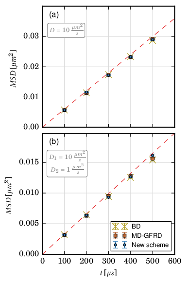
In order to validate the implementation of the MD-GFRD schemes, of the new scheme and of the direct time-step integration scheme used, the mean squared displacement of the particles simulated with the different schemes has been recorded and compared. In Fig. 9, the mean square displacement shows an excellent agreement between the different schemes.
5 Conclusions
We have described a novel multi-scale MD-GFRD scheme to simulate diffusion and interaction of Brownian particles. In a multi-scale MD-GFRD scheme, the propagation of free particles is performed in an event-based fashion via Green’s functions samplings, whilst the reactions and the interactions between particles are simulated via direct time-step integration (here using time-discretized Brownian dynamics, BD).
Multi-scale MD-GFRD has been shown to be several orders of magnitude faster than BD at low particle concentrations. The efficiency of MD-GFRD strongly depends on the density of the system, and previous schemes have been shown to be more efficient than BD up to a molar concentrations of [20, 21]. In crowded systems, free space around particles tends to be scarce and constructing protective domains around them is more difficult. In addition, domains are often burst prematurely by the intrusion of other particles, which is undesirable as it increases the computational effort and the domain making is less parallelizable than direct BD steps or FPKMC/eGFRD extractions. It is thus desirable to optimize the domain making scheme so as to avoid unnecessary premature bursting and improve the computational performance at a given particle concentration.
In the multi-scale MD-GFRD scheme described in this paper, a new domain making algorithm and a way to determine the minimal domain size accurately have been introduced. The new domain making algorithm constructs domains with sizes chosen so as to balance the domain exit times of adjacent particles. In contrast to previous domain selection schemes, this approach involves sampling exit positions, i.e. it looks ahead in time in order to plan domain sizing optimally. In addition, the minimal domain size is proposed to be proportional to the square root of the particle diffusivity, which leads to the existence of smaller domains than in previous implementations. Nonetheless, the domains created with this algorithm are more efficient as they are less likely to burst. Overall, the new scheme exhibits up to an order of magnitude improvement of computational efficiency compared to the previous multi-scale MD-GFRD implementations. Moreover, the new scheme is superior to direct time-step integration for concentrations up to . In future studies, this algorithm will be used as a part of the software ReaDDy to simulate realistic biological systems.
Acknowledgement
The authors gratefully acknowledge funding by Deutsche Forschungsgemeinschaft (SFB 1114/C03 to L.S. and F.N), European Research Commission (starting grant 307494 “pcCell” to F.N.), and the Max Planck Society (International Max Planck Research School CBSC fellowship to L.S.). The authors would like to thank Thomas R. Sokolowski for useful discussions.
Appendix A New domain size scheme
The solution to Eq. (5) has the following two roots:
| (18) |
Assuming that the condition is satisfied, the argument of the square root is nonnegative, resulting in two real-valued solutions. In the following derivations, we study two different cases depending on and .
Firstly, we study , which leads to . In case the discriminant is added the factor that multiplies is clearly higher than one, since diffusion coefficients are always positive, then we would obtain , an unphysical solution. The discriminant must thus be subtracted. Furthermore, imposing the condition , or equivalently , we can verify that if the discriminant is subtracted:
| (19) |
The condition is satisfied if the discriminant is subtracted.
In case , then :
| (20) |
In order to satisfy the condition , the discriminant must have a positive sign. However, the sign of the discriminant has been inverted by the modulus in the denominator, since it comes from the subtraction of the discriminant.
To sum up, only the root obtained by subtracting the discriminant satisfies the condition :
| (21) |
Appendix B values
The minimal domain size is given by eq. (16), where is a parameter that is determined in the beginning of the simulation. An optimal value has been already suggested in Fig. 4. However, that value was selected by taking only the Green’s function solver and the direct time-step integrator into account. In general, it might seem appropriate to insert a penalty for the possibility of a burst and then to slightly rise the value, where the penalty would be higher when a higher number of bursts is expected.
Fig. 10 shows that the optimal value of lies in the range , in agreement with Fig. 4. However, in the system studied here, the effect of varying in on CPU performance is lower than , and essentially any value in this interval can be chosen. was chosen in the simulations shown in Fig. 5.

References
- [1] J. Schöneberg, M. Heck, K.-P. Hofmann, and F. Noé, Biophys. J. 107, 1042 (2014).
- [2] K. Takahashia, S. Tănase-Nicolad, and P. R. ten Wolde, Proceedings of the National Academy of Sciences 107, 2473 (2009).
- [3] R. Erban and S. J. Chapman, Physical Biology 6, 046001 (2009).
- [4] J. van Zon and P. ten Wolde, J. Chem. Phys. 123, 234910 (2005).
- [5] J. Schöneberg et al., Nat. Commun. 8, 15873 (2017).
- [6] D. T. Gillespie, J. Comput. Phys. 22, 403 (1976).
- [7] S. Winkelmann and C. Schütte, J. Chem. Phys. 145, 214107 (2016).
- [8] P. Langevin, Comptes-rendus de l’Académie des sciences 146, 530 (1908).
- [9] S. S. Andrews and D. Bray, Physical biology 1, 137 (2004).
- [10] J. Schöneberg and F. Noé, PLoS ONE 8 (2013).
- [11] J. Schöneberg, A. Ullrich, and F. Noé, BMC Biophysics 7, 11 (2014).
- [12] M. Gunkel et al., Structure 23, 628 (2015).
- [13] A. Ullrich et al., PLoS Comput. Biol. 11, e1004407 (2015).
- [14] S. R. McGuffee and A. H. Elcock, PLoS Comput. Biol. 6, e1000694 (2010).
- [15] J. Biedermann, A. Ullrich, J. Schöneberg, and F. Noé, Biophys. J. 108, 457 (2015).
- [16] T. Opplestrup et al., Phys. Rev. Lett. 97, 230602 (2006).
- [17] T. Oppelstrup et al., Phys. Rev. E 80, 066701 (2009).
- [18] A. Donev et al., J. Comp. Phys. 229, 3214 (2010).
- [19] J. van Zon and P. ten Wolde, Phys. Rev. Lett. 94, 128103 (2005).
- [20] A. Vijaykumar, P. Bolhuis, and P. ten Wolde, J. Chem. Phys. 143, 214102 (2015).
- [21] A. Vijaykumar, T. Ouldridge, P. ten Wolde, and P. Bolhuis, J. Chem. Phys. 146, 114106 (2017).
- [22] J. Schluttig, C. B. Korn, and U. S. Schwarz, Phys. Rev. E 81, 030902 (2010).
- [23] J.-H. Prinz et al., J. Chem. Phys. 134, 174105 (2011).
- [24] G. R. Bowman, V. S. Pande, and F. Noé, editors, An Introduction to Markov State Models and Their Application to Long Timescale Molecular Simulation., volume 797 of Advances in Experimental Medicine and Biology, Springer Heidelberg, 2014.
- [25] M. Sarich and C. Schütte, Metastability and Markov State Models in Molecular Dynamics, Courant Lecture Notes, American Mathematical Society, 2013.
- [26] F. Noé and C. Clementi, J. Chem. Theory Comput. 11, 5002 (2015).
- [27] N. Plattner, S. Doerr, G. D. Fabritiis, and F. Noé, Nat. Chem. 9, 1005 (2017).
- [28] H. Wu, A. S. J. S. Mey, E. Rosta, and F. Noé, J. Chem. Phys. 141, 214106 (2014).
- [29] H. Wu, F. Paul, C. Wehmeyer, and F. Noé, Proc. Natl. Acad. Sci. USA 113, E3221 (2016).
- [30] T. Sokolowski, pp. 48-49, PhD thesis, 2013.
- [31] S. Redner, A Guide to First-Passage processes, Cambridge University Press, 2001.